Statistical properties of subgroups of free groupsThanks: All authors benefitted from the support of the French-Spanish program picasso (project ACI-HF2006-0239). The first and third authors were supported by the ANR (projects blan 07-2_195422 gamma and anr-2010-blan-0204 magnum). The second and fourth authors were supported by MEC (Spain) and the EFRD (EC) through project number MTM2008-01550. The last author was supported by the ESF program AutoMathA and by the ANR (project anr-2010-blan-0202 frec).Thanks: LIPN, Université Paris 13 and CNRS, Institut Galilée, 99, avenue Jean-Baptiste Clément, 93430 Villetaneuse, FranceThanks: School of Mathematics, University of Southampton, University Road, Southampton SO17 1BJ, United KingdomThanks: Institut Gaspard Monge, Université Paris-Est, 77454 Marne-la-Vallée Cedex 2, FranceThanks: Universitat Politecnica de Catalunya, Av. Bases de Manresa 61-73, 08240 Manresa, Catalunya, Spain Thanks: LaBRI, Univ. Bordeaux, 351 cours de la Libération, 33400 Talence, France.

Each finitely generated subgroup of $F(A)$ can be represented uniquely by a finite graph of a particular type, by means of the technique known as Stallings foldings [32]. This representation has been used by many authors, frequently using combinatorial, graph-theoretic notations that slightly differ from those used by Stallings. It is this formalism that we also use, which can also be found in [34, 17, 33, 22]. The procedure of Stallings foldings is informally described at the end of this section.

An $A$-graph is defined to be a pair $\Gamma=(V,E)$ with $E\subseteq V\times A\times V$, such that

• •

  if $(u,a,v),(u,a,v^{\prime})\in E$, then $v=v^{\prime}$;

• •

  if $(u,a,v),(u^{\prime},a,v)\in E$, then $u=u^{\prime}$.

The elements of $V$ are called the vertices of $\Gamma$ and the elements of $E$ are its edges. We say that $\Gamma$ is connected if the underlying undirected graph is connected. If $v\in V$, we say that $v$ is a leaf if $v$ occurs at most once in (the list of triples defining) $E$ and we say that $\Gamma$ is $v$-trim if no vertex $w\neq v$ is a leaf. Finally we say that the pair $(\Gamma,v)$ is admissible if $\Gamma$ is a finite, $v$-trim and connected $A$-graph. Then it is known (see [32, 34, 17, 22]) that:

• •

  Stallings associated with each finitely generated subgroup $H$ of $F(A)$ a unique admissible pair of the form $(\Gamma,1)$, which we call the graphical representation or the Stallings graph of $H$ and write $\Gamma(H)$;

• •

  every admissible pair $(\Gamma,1)$ is the graphical representation of a unique finitely generated subgroup of $F(A)$;

• •

  if $(\Gamma,1)$ is the graphical representation of $H$ and $u$ is a reduced word, then $u\in H$ if and only if $u$ labels a loop at 1 in $\Gamma$ (by convention, an edge $(u,a,v)$ can be read from $u$ to $v$ with label $a$, or from $v$ to $u$ with label $a^{-1}$);

• •

  if $(\Gamma,1)$ is the graphical representation of $H$, then $\textsf{rank}(H)=|E|-|V|+1$;

• •

  finitely generated subgroups $H$ and $K$ are conjugates if and only if the cyclic cores of $\Gamma(H)$ and $\Gamma(K)$ (obtained by repeatedly deleting leaves and the edges they are adjacent to) are equal.

We informally remind the readers of the computation of the graphical representation of a subgroup generated by a subset $B=\{u_{1},\ldots,u_{k}\}$. It consists in building an $(A\sqcup A^{-1})$-graph, changing it into a $A$-graph, then reducing it using foldings. First build a vertex $1$. Then, for every word $u$ of length $n$ in $B$, build a loop with label $u$ from $1$ to $1$, adding $n-1$ vertices. Change every edge $(u,a^{-1},v)$ labeled by a letter of $A^{-1}$ into an edge $(v,a,u)$. Then iteratively identify the vertices $v$ and $w$ whenever there exists a vertex $u$ and a letter $a\in A$ such that either both $(u,a,v)$ and $(u,a,w)$ or both $(v,a,u)$ and $(w,a,u)$ are edges in the graph (the corresponding two edges are folded, in Stallings’ terminology).

The resulting graph $\Gamma$ is such that $(\Gamma,1)$ is admissible and, very much like in the (1-dimensional) reduction of words, it does not depend on the order used to perform the foldings.

Let $S$ be a countable set, the disjoint union of finite sets $S_{n}$ ($n\geq 0$), and let $B_{n}=\bigcup_{i\leq n}S_{i}$. Typically in this paper, $S$ will be the set of Stallings graphs, of partial injections, of reduced words or of $k$-tuples of reduced words, and $S_{n}$ will be the set of elements of $S$ of size $n$. A subset $X$ of $S$ is negligible (resp. generic) if the probability for an element of $B_{n}$ to be in $X$, tends to 0 (resp. to 1) when $n$ tends to infinity; that is, if $\lim_{n}\frac{|X\cap B_{n}|}{|B_{n}|}=0$ (resp. $=1$).

Naturally, the negligibility or the genericity of a subset $X$ of $S$ depends on the layering of $S$ into the $S_{n}$. In particular, if $X$ and its complement are both infinite, then an appropriate partition of $S$ into finite subsets $S_{n}$ will make $X$ negligible, another will make it generic, and indeed, another will be such that $\lim_{n}\frac{|X\cap B_{n}|}{|B_{n}|}=p$ for any fixed $0<p<1$.

Thus, any discussion of negligibility or genericity must clearly specify the distribution that is considered, that is, the choice of the partition $(S_{n})_{n}$.

The distribution usually found in the literature (e.g. [18, 15, 16]) is in fact a distribution on the $k$-tuples $\vec{h}=(h_{1},\ldots,h_{k})$ of reduced words of length at most $n$, where $k$ is fixed and $n$ is allowed to grow to infinity; one then considers the subgroup $H$ generated by $\vec{h}$. We call this distribution word-based.

Let us first record three elementary facts, which can also be found in [15]¹¹ 1 We choose to reiterate the proofs of these results, because we feel that our presentation exhibits more clearly their combinatorial underpinnings.. We denote by $R_{n}$ the set of reduced words of length at most $n$.

The number of reduced words of length $i\geq 1$ is $2r(2r-1)^{i-1}$, so the cardinality of $R_{n}$ is

$\sqcap$$\sqcup$

The proportion of words in $R_{n}$, of length less than or equal to $\alpha n$, is

Since $\alpha-1<0$, it converges to 0 exponentially fast.   $\sqcap$$\sqcup$

Let $\vec{h}=(h_{1},\ldots,h_{k})$ be a tuple of reduced words and let $\mu>0$ such that $\min|h_{i}|>2\lceil\mu\rceil$. We denote by $\textsf{Pref}_{\mu}(\vec{h})$ the set of prefixes of length at most $\lceil\mu\rceil$ of the $h_{i}$ and $h_{i}^{-1}$.

The complement in $R_{n}^{k}$ of the set of $k$-tuples described in the statement is the union of the set $Y$ of $k$-tuples $\vec{h}$ where $\min|h_{i}|\leq 2\lceil\lambda n\rceil$, and of the set $Z$ of $k$-tuples where $\min|h_{i}|>2\lceil\lambda n\rceil$ and the set of prefixes of length $\lceil\lambda n\rceil$ of the $h_{i}$ and $h_{i}^{-1}$ has at most $2k-1$ elements. Since $2\lambda<1$, the set $Y$ is exponentially negligible by Fact 3.2 and we now concentrate on $Z$.

For each integer $2\lceil\lambda n\rceil<m\leq n$, let $Z_{m}$ be the set of $k$-tuples in $Z$, such that $\min|h_{i}|=m$. Then

Summing these inequalities for all $2\lceil\lambda n\rceil<m\leq n$, we find

As a result, the proportion of $k$-tuples in $Z$ is at most

for some constant $C$ depending only on $k$ and $r$. Thus, this proportion converges to 0 exponentially fast.   $\sqcap$$\sqcup$

Let $0<\alpha<1$ and $0<\lambda<\frac{\alpha}{2}$, and for each $n$, let $Y_{\alpha,\lambda,n,k}$ be the set of $k$-tuples $\vec{h}=(h_{1},\ldots,h_{k})\in R_{n}^{k}$ such that $\min|h_{i}|>\alpha n$ and the prefixes of the $h_{i}$ and $h_{i}^{-1}$ of length $\lceil\lambda n\rceil$ are pairwise distinct. Facts 3.2 and 3.3 show that the proportion of elements of $R_{n}^{k}$ in $Y_{\alpha,\lambda,n,k}$ converges to 1 exponentially fast: in the search for exponentially generic properties of subgroups, we can restrict our attention to the tuples in $Y_{\alpha,\lambda,n,k}$ and to the subgroups they generate.

The following observation is the basis for our exponential genericity proofs, in the context of the word-based distribution.

This leads to the following results. Propositions 3.6 and 3.8 first appeared in a paper by Jitsukawa [15]. They are direct consequences of earlier analogous results (counting cyclic words instead of words) due to Arzhantseva and Ol’shanskiĭ [2, Lemma 3].

Let $\alpha,\lambda$ satisfy $0<2\lambda<\alpha<1$. As observed above, it suffices to show that if $\vec{h}\in Y_{\alpha,\lambda,n,k}$, then $H=\langle\vec{h}\rangle$ has rank $k$. In that case, using Fact 3.5, we find that $\Gamma(H)$ is formed of a central part and $k$ outer loops.

The central part is a tree and like all trees, the number of its edges is 1 less than the number of its vertices. With the notation of Fact 3.5, the number of additional vertices (resp. edges) in the outer loops is $\sum_{i}(|m_{i}|-1)$ (resp. $\sum_{i}|m_{i}|$). Therefore, in $\Gamma(H)$, we have $|E|-|V|+1=k$ and hence $\textsf{rank}(H)=k$ (see Section 2.1).   $\sqcap$$\sqcup$

Since the first $k$ components of a $(k+k^{\prime})$-tuple of elements of $R_{n}$ are independent from the $k^{\prime}$ last components, and since such a $(k+k^{\prime})$-tuple exponentially generically generates a subgroup of rank $k+k^{\prime}$ (Proposition 3.6), we find that a $k$-tuple and an $k^{\prime}$-tuple of elements of $R_{n}$ exponentially generically generate their free product. This in turn implies the other properties.   $\sqcap$$\sqcup$

Proposition 3.7 shows that two $k$-tuples of elements of $R_{n}$ exponentially generically generate distinct subgroups. Proposition 3.8 is a little more precise.

If $\langle\vec{h}\rangle=\langle\vec{h}^{\prime}\rangle$, then the graphs $\Gamma\langle\vec{h}\rangle$ and $\Gamma\langle\vec{h}^{\prime}\rangle$ are equal. In particular, their central parts, formed by the vertices at distance at most $\lceil\lambda n\rceil$ from the distinguished vertex, coincide. Fact 3.5 shows that if $\vec{h}\in Y_{\alpha,\lambda,n,k}$, then $\Gamma\langle\vec{h}\rangle$ completely determines all the $k$-tuples $\vec{h}^{\prime}\in Y_{\alpha,\lambda,n,k}$ such that $\Gamma\langle\vec{h}^{\prime}\rangle=\Gamma\langle\vec{h}\rangle$, and that they coincide with $\vec{h}$ up to the order of the elements and the direction in which the outer loops are read.   $\sqcap$$\sqcup$

Proposition 3.8 shows that, if we consider the class $S_{\alpha,\lambda,n,k}$ of subgroups generated by $k$-tuples in $Y_{\alpha,\lambda,n,k}$, then each subgroup occurs the same number of times, namely $2^{k}k!$. Randomly choosing a $k$-tuple in $Y_{\alpha,\lambda,n,k}$ yields therefore a random subgroup in $S_{\alpha,\lambda,n,k}$, and the proportion of these subgroups among all subgroups generated by a $k$-tuple of words of length at most $n$ tends to $1$ exponentially fast.

The uniform distribution on the set of size $n$ Stallings graphs was analyzed by Bassino, Nicaud and Weil [3]. Here we summarize the principles of this distribution and the features which will be used in this paper.

We already noted that in Stallings graphs, each letter labels a partial injection on the vertex set: in fact, a Stallings graph can be viewed as a collection $(f_{a})_{a\in A}$ of partial injections on an $n$-element set, with a distinguished vertex, and such that the resulting graph (with an $a$-labeled edge from $i$ to $j$ if and only if $j=f_{a}(i)$) is connected and has no vertex of degree 1, except perhaps the distinguished vertex. We may even assume that the $n$-element set in question is $[n]=\{1,\ldots,n\}$, with 1 as the distinguished vertex, see [3, Section 1.2] for a precise justification. In particular, the automorphism group of an admissible pair $(\Gamma,1)$ is always trivial.

One shows [3, Corollary 2.7] that the probability that an $A$-tuple $(f_{a})_{a\in A}$ of partial injections on $[n]$ induces a Stallings graph tends to 1 as $n$ tends to infinity, and the problem of randomly generating a Stallings graph then reduces (via an efficient rejection algorithm, see [3, Section 3]) to the problem of efficiently generating a random partial injection on $[n]$. This view of a Stallings graph as an $A$-tuple of partial injections on $[n]$ is central in our analysis.

The maximal orbits of a partial injection $f$ (equivalently: the connected components of the function graph of $f$) can be of two kinds: cycles – where each element is both in the domain and in the range of $f$ – and sequences. The size of each of these components is defined to be the number of vertices which they contain. It is this combinatorial view of partial injections – as a disjoint union of cycles and sequences –, which is at the heart of the random generation algorithm, obtained using the so-called recursive method [26, 12].

The distribution of sizes of components is studied in [3, Section 3], as well as the distribution of cycles vs. sequences among size $k$ components. The random generation algorithm consists in drawing a size of component, say $k$, according to the relevant distribution; then drawing whether this size $k$ component is a cycle or a sequence; and finally drawing a partial injection on the remaining $n-k$ elements [3, Section 3.1]. This results in a partial injection on an $n$-element set, and we need only add a random numbering (1 through $n$) of the elements of that set.

However complex the method may seem, it guarantees a uniform distribution among all size $n$ partial injections, it is easy to implement and its average time complexity is linear (in the RAM model; it is $\mathcal{O}(n^{2}\log n)$ under the bit-cost assumption) [3, Section 3.3].

To further discuss partial injections and other combinatorial structures, we use the notion of exponential generating series, written EGS. If $\mathcal{S}$ is a class of finite discrete structures such that there are finitely many $\mathcal{S}$-structures of each size, let $S_{n}$ be the number of $\mathcal{S}$-structures of size $n$. The EGS of $\mathcal{S}$ is the formal power series $S(z)=\sum_{n\geq 0}\frac{S_{n}}{n!}z^{n}$.

Let $I(z)=\sum_{n\geq 0}\frac{I_{n}}{n!}z^{n}$ be the EGS of partial injections. Bassino, Nicaud and Weil show the following [3, Section 2.1 and Proposition 2.10].

This result is obtained by means of deep theorems from analytic combinatorics. The same methods can be used to study the asymptotic behavior of particular parameters, such as the number of sequences of a partial injection. This parameter is directly connected with the number of edges in the Stallings graph formed by the partial injections $f_{a}$ ($a\in A$), which leads to the following result [3, Lemma 2.11 and Corollary 4.1].

Thus, in the discussion of statistical properties of finitely generated subgroups of a (fixed) free group $F_{r}$, we have two distributions at our disposal. One, the word-based distribution, is governed by two parameters: the number of generators and their maximum length, the former fixed and the latter allowed to tend to infinity. The other, the graph-based distribution, is governed by a single parameter: the size of the Stallings graph.

We first observe that our discussion of the graph-based distribution (as well as the results in [3]) is in terms of spheres rather than balls: as we saw in the Section 2.2.2, the (exponential) negligibility or genericity results obtained in that setting are sufficient. In contrast, the existing literature on the word-based distribution is in terms of balls, as is our description in Section 3.1 above.

The graph-based as well as the word-based distribution allow the discussion of properties of subgroups (of subgroups of a fixed rank $k$ in the word-based case). There is of course no reason why a property that is generic or negligible in one distribution should have the same frequency in the other.

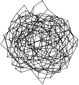
Our two distributions are indeed very different. How different is illustrated in Figure 1, which shows a “random” size 200 Stallings graph and the Stallings graph of the subgroup of $F_{2}$ generated by a “random” 5-tuple of words of length at most 40 (which has close to 200 vertices). This figure provides the intuition to exhibit properties of subgroups that are negligible in one distribution and generic in the other.

It is not difficult to come up with such properties. It is the case, for instance, of the property to have rank $\ell$, for a fixed integer $\ell\geq 1$. In the graph-based distribution, this property is negligible as a consequence of Proposition 3.10 (see [3, Corollary 4.2]). In contrast, it is exponentially generic in the word-based distribution of $\ell$-generated subgroups, see Proposition 3.6. For the same reason, it is exponentially negligible in the word-based distribution of $k$-generated subgroups with $k\neq\ell$.

The properties of malnormality and purity, discussed in Section 4, provide more complex examples of this sort.

Jitsukawa shows that malnormality is a generic property in free groups [15, Theorem 4 and Lemma 6]. His arguments can be extended to show that it is exponentially generic.

In view of Lemma 4.1, we also have the following result.

We now proceed to prove Theorem 4.3. The proof relies on the two following lemmas, which provide an analogue of a small cancellation property for tuples of reduced words. These lemmas constitute a variant of the results of Gromov [14, 0.2.A] for tuples of cyclic words, proved also by Champetier [8, 9] and by Arzhantseva and Ol’shanskiĭ [2, Lemma 3].

We can now prove Theorem 4.3.

Let $0<\alpha<1$ and $0<\lambda<\frac{\alpha}{4}$. Let $\vec{h}=(h_{1},\ldots,h_{k})$. Exponentially generically, we have $\min|h_{i}|>\alpha n$ and the prefixes of length $\lceil\lambda n\rceil$ of the $h_{i}$ and $h_{i}^{-1}$ are pairwise distinct (Facts 3.2 and 3.3). In addition, exponentially generically, no word of length at least $\frac{\alpha-4\lambda}{2}n$ has distinct occurrences as a factor of the $h_{i}$ and the $h_{i}^{-1}$ (Lemmas 4.5 and 4.6).

Let us now assume that $\vec{h}$ satisfies all these properties. Then $\Gamma=\Gamma(\langle\vec{h}\rangle)$ is composed of a central part, which is a tree containing the distinguished vertex and all the vertices corresponding to the prefixes of the $h_{i}$ and $h_{i}^{-1}$ of length up to $\lceil\lambda n\rceil$, and of outer loops whose labels are factors of the $h_{i}$ (or the $h_{i}^{-1}$, depending on the direction in which they are read), see Fact 3.5.

Any loop in $\Gamma$ must visit the central part of $\Gamma$ at least once, and run along at least one of the outer loops. Let us now assume that a word $u$ labels two distinct loops in $\Gamma$. Up to conjugation of $u$, we can assume that the base point of the first loop is in the central part of $\Gamma$. Then $u$ has a factor $v$ of length $\lceil\alpha n\rceil-2\lceil\lambda n\rceil$, which is a factor of some $h_{i}$ or $h_{i}^{-1}$. The other occurrence of a loop labeled $u$ reveals another path in $\Gamma$ labeled $v$. This path may not be entirely in an outer loop, but if it is not, then it visits the central part of $\Gamma$ only once, so it has a factor $v^{\prime}$ of length at least $\frac{\alpha-4\lambda}{2}n$ in an outer loop, and hence in one of the $h_{i}$ or $h_{i}^{-1}$. This word $v^{\prime}$ has distinct occurrences as a factor of the $h_{i}$ and the $h_{i}^{-1}$, a contradiction.   $\sqcap$$\sqcup$

In contrast, we show that malnormality and purity are negligible in the graph-based distribution.

By Lemma 4.1, this implies the following

To prove Theorem 4.7, we observe that if $H$ is a finitely generated subgroup of $F_{r}$ and a cycle of length at least 2 in $\Gamma(H)$ is labeled by a power of some letter $a$, then $H$ is not pure (Proposition 4.2). Therefore, if a subgroup is pure, then the partial injection determined by each letter in $A$ has only sequences and length 1 cycles.

Thus Theorem 4.7 follows directly from the following proposition.

Our proof of Proposition 4.9 uses Hayman’s theorem, discussed in Section 4.2.1 below.

References

- [1] Goulnara N. Arzhantseva. A property of subgroups of infinite index in a free group. Proc. Amer. Math. Soc., 128(11):3205–3210, 2000.
- [2] Goulnara N. Arzhantseva and Alexander Yu. Ol′shanskiĭ. Generality of the class of groups in which subgroups with a lesser number of generators are free. Mat. Zametki, 59(4):489–496, 638, 1996.
- [3] Frédérique Bassino, Cyril Nicaud, and Pascal Weil. Random generation of finitely generated subgroups of a free group. Internat. J. Algebra Comput., 18(2):375–405, 2008.
- [4] Gilbert Baumslag, Alexei Myasnikov, and Vladimir Remeslennikov. Malnormality is decidable in free groups. Internat. J. Algebra Comput., 9(6):687–692, 1999.
- [5] Jean-Camille Birget, Stuart Margolis, John Meakin, and Pascal Weil. PSPACE-complete problems for subgroups of free groups and inverse finite automata. Theoret. Comput. Sci., 242(1-2):247–281, 2000.
- [6] Steven A. Bleiler and Amelia C. Jones. The free product of groups with amalgamated subgroup malnormal in a single factor. J. Pure Appl. Algebra, 127(2):119–136, 1998.
- [7] Robert G. Burns. On finitely generated subgroups of free products. J. Austral. Math. Soc., 12:358–364, 1971.
- [8] Christophe Champetier. Propriétés génériques des groupes de présentation finie. Ph.D. Thesis, Université Lyon 1 (1991).
- [9] Christophe Champetier. Propriétés statistiques des groupes de présentation finie. J. Adv. Math., 116(2):197–262, 1995.
- [10] Louis Comtet. Advanced combinatorics. D. Reidel Publishing Co., Dordrecht, enlarged edition, 1974. The art of finite and infinite expansions.
- [11] Philippe Flajolet and Robert Sedgewick. Analytic combinatorics. Cambridge University Press, Cambridge, 2009.
- [12] Philippe Flajolet, Paul Zimmerman, and Bernard Van Cutsem. A calculus for the random generation of labelled combinatorial structures. Theoret. Comput. Sci., 132(1-2):1–35, 1994.
- [13] Stephen M. Gersten. Intersections of finitely generated subgroups of free groups and resolutions of graphs. Invent. Math., 71(3):567–591, 1983.
- [14] Mikhail Gromov. Hyperbolic groups. In Essays in group theory, S.M. Gersten ed., pages 75–265. Springer, 1987.
- [15] Toshiaki Jitsukawa. Malnormal subgroups of free groups. In Computational and statistical group theory (Las Vegas, NV/Hoboken, NJ, 2001), volume 298 of Contemp. Math., pages 83–95. Amer. Math. Soc., Providence, RI, 2002.
- [16] Ilya Kapovich, Alexei Miasnikov, Paul Schupp, and Vladimir Shpilrain. Generic-case complexity, decision problems in group theory, and random walks. J. Algebra, 264(2):665–694, 2003.
- [17] Ilya Kapovich and Alexei Myasnikov. Stallings foldings and subgroups of free groups. J. Algebra, 248(2):608–668, 2002.
- [18] Ilya Kapovich, Paul Schupp, and Vladimir Shpilrain. Generic properties of Whitehead’s algorithm and isomorphism rigidity of random one-relator groups. Pacific J. Math., 223(1):113–140, 2006.
- [19] Abraham Karrass and Donald Solitar. The free product of two groups with a malnormal amalgamated subgroup. Canad. J. Math., 23:933–959, 1971.
- [20] Olga Kharlampovich and Alexei Myasnikov. Hyperbolic groups and free constructions. Trans. Amer. Math. Soc., 350(2):571–613, 1998.
- [21] Stuart Margolis, Mark Sapir, and Pascal Weil. Closed subgroups in pro- topologies and the extension problem for inverse automata. Internat. J. Algebra Comput., 11(4):405–445, 2001.
- [22] Alexei Miasnikov, Enric Ventura, and Pascal Weil. Algebraic extensions in free groups. In Geometric group theory, Trends Math., pages 225–253. Birkhäuser, Basel, 2007.
- [23] Igor Mineyev. Submultiplicativity and the Hanna Neumann conjecture. Annals of Math., 175(1): 393–414, 2011.
- [24] Igor Mineyev. Groups, graphs, and the Hanna Neumann Conjecture. Preprint, 10 pages, www.math.uiuc.edu/~mineyev/math/art/gr-gr-shnc.pdf
- [25] Alexei Myasnikov, Vladimir Shpilrain, and Alexander Ushakov. Group-based cryptography. Advanced Courses in Mathematics. CRM Barcelona. Birkhäuser Verlag, Basel, 2008.
- [26] Albert Nijenhuis and Herbert S. Wilf. Combinatorial algorithms. Academic Press Inc. [Harcourt Brace Jovanovich Publishers], New York, second edition, 1978. For computers and calculators, Computer Science and Applied Mathematics.
- [27] Yann Ollivier. A January 2005 invitation to random groups. Ensaios Matemáticos, 10. Sociedade Brasileira de Matemática, 2005.
- [28] Alexander Yu. Ol′shanskiĭ. Almost every group is hyperbolic. Internat. J. Algebra Comput., 2(1):1–17, 1992.
- [29] Abdó Roig, Enric Ventura, and Pascal Weil. On the complexity of the Whitehead minimization problem. Internat. J. Algebra Comput., 17(8):1611–1634, 2007.
- [30] Mark Sapir. Residual properties of 1-relator groups. Technical report, arXiv:1001.2829v1, 2010.
- [31] Mark Sapir and Iva Spakulova. Almost all one-relator groups with at least three generators are residually finite. Technical report, arXiv:0809.4693v2, 2009.
- [32] John R. Stallings. Topology of finite graphs. Invent. Math., 71(3):551–565, 1983.
- [33] Nicholas W. M. Touikan. A fast algorithm for Stallings’ folding process. Internat. J. Algebra Comput., 16(6):1031–1045, 2006.
- [34] Pascal Weil. Computing closures of finitely generated subgroups of the free group. In Algorithmic problems in groups and semigroups (Lincoln, NE, 1998), Trends Math., pages 289–307. Birkhäuser Boston, Boston, MA, 2000.