Hamiltonian motions of plane curves and formation of singularities and bubbles
Abstract
A class of Hamiltonian deformations of plane curves is defined and studied. Hamiltonian deformations of conics and cubics are considered as illustrative examples. These deformations are described by systems of hydrodynamical type equations. It is shown that solutions of these systems describe processes of formation of singularities (cusps, nodes), bubbles, and change of genus of a curve.
pacs
02.30.Ik, 02.40.Re, 02.30.Jrams
37K10, 14H701 Introduction
Dynamics of curves and interfaces is a key ingredient in various important phenomena in physics and theories in mathematics (see e.g. [2, 5, 24, 31]).
Special class of deformations of curves described by integrable equations has attracted a particular interest. It has been studied in a number of papers (see [3, 4, 6, 7, 9, 12, 16, 17, 19, 15, 20, 21, 22, 23, 25, 26, 27, 29, 30, 36, 37] and references therein).
Approaches used in these papers differ, basically, by the way how the evolution of a curve is fixed. In papers [6, 9, 12, 25, 23, 30] the motion of the curve is defined by requirement that the time derivative of position vector of a curve is a linear superposition of tangent and (bi)normal vectors with a certain specification of coefficients in this superposition. Deformations considered in papers [3, 7, 20, 21, 36] are defined, basically, by the corresponding Lax pair. Within the study of Laplacian growth problem [4, 22, 26, 29, 36, 37, 27] the time evolution of the interface is characterized by the dynamics of the Schwartz function of a curve prescribed by the Darcy law.
Semiclassical deformations of algebraic curves analyzed in [16, 15, 17] are fixed by the existence of a specific generating function constructed a Lenard scheme.
Finally, the coisotropic deformations introduced in [19] are defined by the requirement that the ideal of the deformed curve is a Poisson ideal.
In the present paper a novel class of deformations of plane curves is considered. For such deformations the function which defines a curve in the plane obeys an inhomogeneous Liouville equation with and deformation parameters playing the role of independent variables. These deformations are referred as the Hamiltonian deformations (motions) of a curve since the coefficients in the linear equation are completely fixed by the single function playing a role of Hamiltonian for time dynamics. Equivalently Hamiltonian deformations can be defined as those for which an ideal of a deformed curve is invariant under the action of the vector field . For algebraic plane curves Hamiltonian deformations represent a particular class of coisotropic deformations introduced in [19].
Here we concentrate on the study of Hamiltonian dynamics of plane quadrics (conics) and cubics. This dynamics is described by integrable systems of hydrodynamical type for the coefficients of polynomials defining algebraic curves with the dKdV, dDS, dVN, (2+1)-dimensional one-layer Benney system and other equations among them. It is shown that particular solutions of these systems describe formation of singularities (cusps, nodes) and bubbles on the real plane.
The paper is organized as follows. General definition and interpretations are given in section 2. Hamiltonian deformations of plane quadrics are studied in section 3. As particular examples one has deformations of circle described by dispersionless Veselov-Novikov (dVN) equation and deformations of an ellipse given by a novel system of equations. Section 4 is devoted to Hamiltonian deformations of plane cubics. An analysis of formation of singularities for cubics and genus transition is given. In section a connection between singular cubics and Burgers-Hopf equation is considered. In section we discuss briefly deformations of a quintic. Possible extensions of the approach presented in the paper are noted in section .
2 Definition and interpretation
So let the plane curve be defined by the equation
| (1) |
where is a function of local coordinates on the complex plane . To introduce deformations of the curve (1) we assume that depends also on the deformation parameters .
Definition 1
If the function obeys the equations
| (2) |
with certain function and a function , where is the Poisson bracket
| (3) |
then it is said that the function as the function of , , and defines Hamiltonian deformations of the curve (1).
To justify this definition we first observe that equation (2) is nothing else than inhomogeneous Liouville equation which is well-known in classical mechanics. On the r.h.s. of equation (2) vanishes and, hence,
| (4) |
where is the Hamiltonian vector field in the space with coordinates . Thus Hamiltonian deformations of the curve (1) generated by can be equivalently defined as those for which the function obeys the condition (4).
Following the standard interpretation of the Liouville equation in the classical mechanics one can view equations (2) and (4) as
| (5) |
and
| (6) |
where the total derivative is calculated along the characteristics of equation (2) defined by Hamiltonian equations
| (7) |
For a given irreducible curve () a function is not defined uniquely. Indeed, for any function the function defines the same curve (1). Then, equation (2) takes the form
| (8) |
where
| (9) |
while the condition (4) remains unchanged. Thus, the freedom in form of given by (9) is just a gauge type freedom. For given the choice of as a solution of the equation
| (10) |
gives . So there exists a gauge at which equation (2) is homogeneous one. The drawback of such “gauge” is that in many cases equation (1) has no simple, standard form in this gauge.
Gauge freedom observed above becomes very natural in the formulation based on the notion of ideal of a curve. Ideal of an irreducible curve (1) consists of all functions of the form (see e.g. [11]). In these terms Hamiltonian deformations of a curve can be characterized equivalently by
Definition 2
Hamiltonian deformations of a curve generated by a function are those for which the ideal of the deformed curve is closed under the action of the vector field , i.e.
| (11) |
Definition of the Hamiltonian deformation in this form clearly shows the irrelevance of the concrete form of function in equation (2). Moreover such formulation reveals also the nonuniqueness in the form of for the same deformation. Indeed, for the family of Hamiltonians where is arbitrary element of (i.e. ) one has equation (2) with the family of functions of the form . Hence, equations and and corresponding equations (11) coincide. This freedom ( where is an arbitrary function) in the choice of Hamiltonians is associated with different possible evaluations of on the curve . In practice it corresponds to different possible resolutions of the concrete equation (1) with respect to one of the variables ( or ). This freedom serves to choose simplest and most convenient form of Hamiltonian .
For algebraic curves, i.e. for functions polynomial in , Hamiltonian deformations of plane curves represent themselves a special subclass of coisotropic deformations of algebraic curves in three dimensional space considered in [19].
In three dimensional space the curve is defined by the system of two equations
| (12) |
where are deformation parameters. Its coisotropic deformation is fixed by the condition [19]
| (13) |
where is the canonical Poisson bracket in . It is easy to see that with the choices
, and the condition (13) is reduced to (4) where .
In general, Hamiltonian deformations of the plane curve are parameterized by three independent variables , and . If one variable is cyclic (say , i.e. and, hence, ) then deformations are described by dimensional equations.
3 Deformations of plane quadrics
In the rest of the paper we will consider Hamiltonian deformations of complex algebraic plane curves. We begin with quadrics defined by equation
| (14) |
where are functions of the deformation parameters . Choosing
| (15) |
one gets the system of six equations of hydrodynamical type. This system has several interesting reductions. One is associated with the constraint , , , and and are constants. It is given by the system
| (16) |
At , , it is the dimensional generalization of the one-layer Benney system proposed in [21, 38]
| (17) |
The curve is the hyperbola and the solutions of the system (17) describe deformations of the hyperbola. The simplest solution of the system is given by
| (18) |
The corresponding evolution of the hyperbola is shown in fig. 1.
 |
 |
 |
At , the system (16) becomes the dispersionless Davey-Stewardson (dDS) system considered in [16]. It describes a class of Hamiltonian motions of hyperbola.
For cubic given by
| (19) |
the condition (4) gives rise to a pretty long system of equations. This system admits several distinguished reductions.
Under the constraint , , , we obtain
| (20) |
which is the well-known dispersionless Kadomtsev-Petviashvilii (dKP) equation (see e.g. [20, 14, 38]). It describes Hamiltonian deformations of a parabola .
For the reduction , , , one has the system
| (21) |
that is the dispersionless Veselov-Novikov equation [20]. It gives us Hamiltonian deformations of a circle .
Another interesting reduction describes deformations of an ellipse
| (22) |
i.e. the quadric (14) with , , , and . Considering particular Hamiltonian (19) with , one has the following new system of equations
| (23) |
For the system (23) equation (2) is of the form
| (24) |
where
| (25) |
Solutions of the system (23) describe various regimes in Hamiltonian motions of the ellipse. In particular, for the initial data given by one has deformations of a circle into ellipse.
For and the system (23) admits the reduction . At , the corresponding system coincides with dVN equation (21) modulo the substitutions , and . We note that the last change of is suggested by the transformation of the type discussed in section from the Hamiltonian for the system (23) to the Hamiltonian for the dVN equation.
In the case of cyclic variable the last three equations (23) give
| (26) |
while the first two equations take the form ()
| (27) |
The Hamiltonian becomes . Without loss of generality we choose . Introducing new variables and , one rewrites the (1+1) dimensional system (27) as
| (28) |
Finally using the eccentricity of an ellipse, one gets the system
| (29) |
which describes Hamiltonian deformations of an ellipse in a pure geometrical terms.
The system (28) represents a particular example of the two component (1+1)-dimensional systems of hydrodynamical type (with arbitrary function ). It is well known that such systems are linearizable by a hodograph transformation , (see e.g. [7]). In our case the corresponding linear system is
| (30) |
This fact allows us to construct explicitly wide class of solutions for the system (28).
At the system (28) is the dispersionless limit of the Hirota-Satsuma system [13]. It has a simple polynomial solution
| (31) |
which provide us with deformation of a circle () into an ellipse shown in figure 2.
 |
 |
 |
4 Deformations of plane cubic curve
Hamiltonian deformations of plane cubics exhibit much richer and interesting structure.
The general form of the plane cubic is (see e.g [11])
| (32) |
and dimensional coisotropic deformations of plane cubics have been considered in the paper [19] where corresponding hydrodynamical type system have been derived. Here we will concentrate on the analysis of the formation of singularities and bubbles for the real section of cubic curves described by particular solutions of these systems. To this end we restrict ourself to the dimensional deformations which correspond to the case of cyclic variable and the reduction . Thus, denoting and , one has the cubic curve
| (33) |
The particular choice of as
| (34) |
gives rise to the following system
| (35) |
which is the well known three-component dispersionless KdV system (see [8, 15]). The system (35) describes the Hamiltonian (coisotropic) deformations of the curve (33). Recall that the moduli of the elliptic curve (33) are given by [34]
| (36) |
while the discriminant is
| (37) |
The elliptic curve has singular points and, hence, become rational (genus zero) at the points where .
We note also that in this case equation (2) is
| (38) |
We will analyze polynomial solutions of the system (35). The simples one, linear in and , is
| (39) |
where are arbitrary constants. With the choice , and one has
| (40) |
Equation (33) in this case is
| (41) |
and discriminant becomes
| (42) |
So for this solution deformation parameters and coincide with the moduli and .
On the curve
| (43) |
in the plane (fig. 3) which has the standard parameterization
| (44) |
the elliptic curve (33) is singular, i.e.
| (45) |

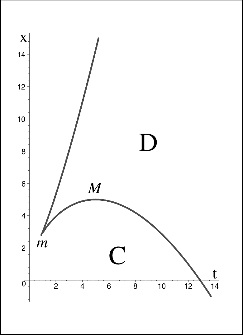
The curve (43) divides the plane in two different domains (fig. 3). In the domain D the discriminant and, hence, the real section of the elliptic curve is disconnected while in the domain C () it is connected. The genus of the curve in both domains is equal to . On the curve (43) it vanishes.
Numerical analysis shows that the transition from the connected to disconnected curve (and viceversa) may happen in three qualitatively different ways shown in the figures (4), (6), and (5) depending on the sign of on the curve (43).
 |
 |
 |
 |
 |
 |
 |
 |
 |
Figure (4) represents the evolution of the real section of the curve (41) in the case when deformation parameters change along the line . Transition from connected to disconnected (with bubble) curve goes through the formation of a double point (node) at . At (fig. 5) the bubble grows up from the point which appears at . From the complex viewpoint the above two regimes are the same. They are related to each other by the involution of the curve (41). Transition through the line at is the limiting case of the above transitions. The formation (or annihilation) of a bubble goes through the formation of the cusp (figure 6). In the figures 4,5,6 and others the plots are ordered in the way to describe transition from connected to disconnected curve. The processes of annihilation and creation of a bubble are converted to each other by a simple change of sign of Hamiltonian.
Richer transition phenomena are observed for the solution (39) with , i.e.
| (46) |
In this case the curve is given by
| (47) |
and the discriminant is
| (48) |
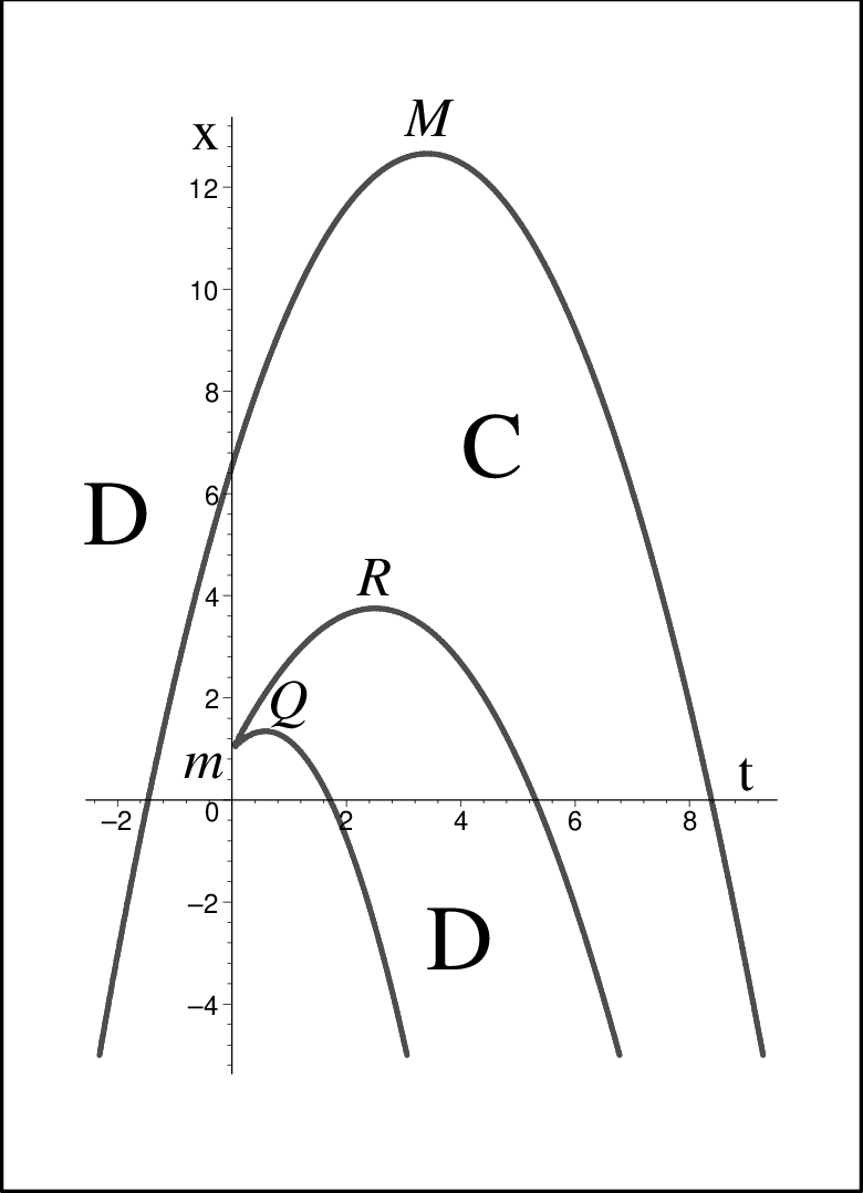
The “phase diagram” (with the curve ) is given in figure (7).
Transition across the curve at and are qualitatively the same as shown in figures 4 and 5. New regime occurs for the transition points with . In this case changing deformation parameters along the line one has the process of formation of the bubble then its absorption and again formation fig. 8.
 |
 |
 | ||
 |
 |
 |
A new behavior appears in this evolution. Starting from a connected curve, a bubble borns and grows far from the boundary until it is connected with the wall through a node. After that the node is desingularized and the (real section) of the curve returns connected. Then, always through a node, a bubble is generated again by the boundary and never comes back.
For the particular choice the elliptic curve becomes
| (50) |
and the discriminant is
| (51) |
The “phase diagram” containing the six order curve is presented in figure (9).
For such deformation of the elliptic curve one observes much richer structure of transition regimes. At the curve remain disconnected for all values of deformation parameters. At the transition involves the absorption and the recreation of a bubble. For the transition involves a double absorption and creation of a bubble. At one has the replication of this regime. For the transition process goes through a complicated oscillation depicted in figure 10 of the bubble interacting with the wall by means of many different nodal critical points.
 |
 |
 | ||
 |
 |
 | ||
 |
 |
 | ||
 |
 |
 |
The above simple examples demonstrate the richness of possible transition processes between connected and disconnected (with a bubble) real sections of elliptic curve described by the system (35).
5 Singular elliptic curve and Burgers-Hopf equation
For all processes of formation and annihilation of bubbles described in the previous section the elliptic curve passes through the “singular point” with at which the curve becomes degenerated (rational). For example, for the simplest solution (40) the elliptic curve assumes the form (45) for the deformation parameters obeying equation (43). The cubic curve (45) is degenerated and possesses a double point for and a cusp for (see e.g. [34]).
More generally, an elliptic curve written in terms of moduli, i.e.
| (52) |
is degenerated if . In this case the curve (52) can be presented in the form
| (53) |
where is the uniformizing variable defined by and .
Singular cubic curve (53) has a well known rational parameterization
| (54) |
Indeed, introducing the variable by relation
| (55) |
one represents equation (53) as
| (56) |
Two equations (55) and (56) are obviously equivalent to (54).
The parameterization (54) clearly indicates the interrelation between the degenerated cubic curve (53) and the Burgers-Hopf (dispersionless Korteweg-de Vries) equation
| (57) |
Equation (57) is known to be equivalent to the compatibility condition for two Hamilton-Jacobi equations (see e.g. [14, 21, 38])
| (58) |
In our approach equation (57) describes the Hamiltonian deformations of the parabola generated by the Hamiltonian or coisotropic deformations of the common points of the curves ([19])
| (59) |
with the standard Poisson bracket . Thus the auxiliary problem (59) for equation (57) represents nothing else than the parameterization (54) of the cubic curve (53). So, any solution of the Burgers-Hopf equation (57) provides us with the family of cubic curves (53) parameterized by the variables and . The solution
| (60) |
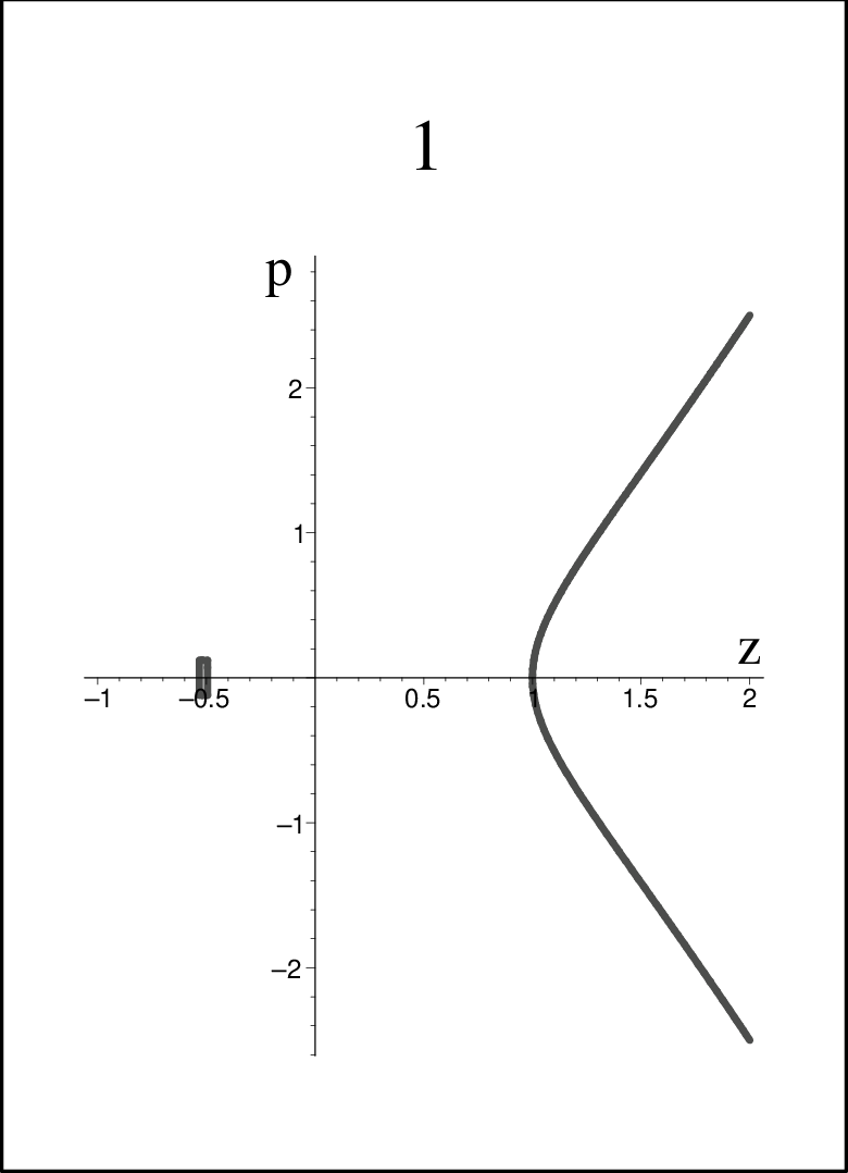
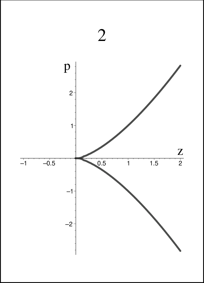
of equation (57) ( is a constant) describes simple Hamiltonian deformation of the degenerated cubic (53) shown in figure (11).
 |
 |
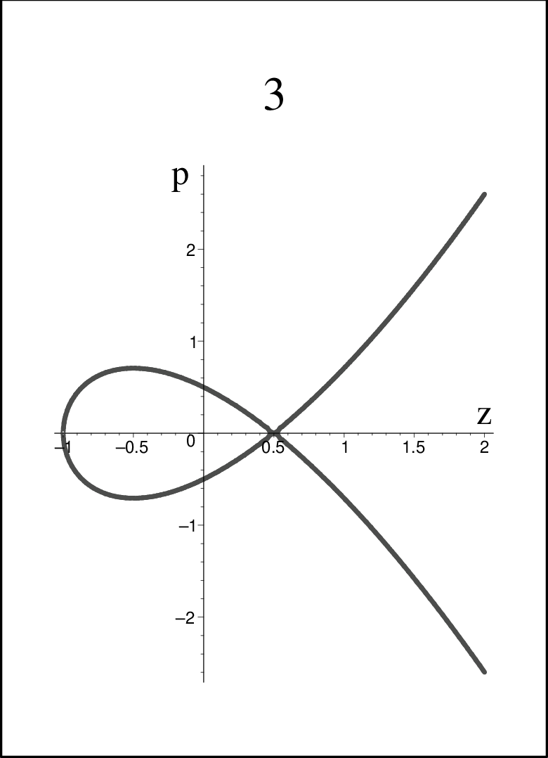 |
The deformation (60) connects singular points of different regimes shown in the figures 4,5,6, i.e. curve with a separate point, cusp and node. This observation shows the relevance of the Burgers-Hopf (dKdV) equation for the description of the singular sector in the process of deformation of elliptic curves. Within the study of the Laplace growth process this fact has been observed earlier in papers [4, 22, 26].
The inverse process of desingularization on the degenerated cubic curve, i.e. the passage from the curve (53) to the curve (33) can be viewed at least in two different ways. One is based on the Birkhoff stratification for the Burgers-Hopf hierarchy. In this approach the passage from (53) to (33) is associated with the transition from the big cell of the Sato Grassmannian to the first stratum [15]. Another approach discussed in [4, 22, 26] suggests the dispersive regularization. Possible interconnection between these two approaches still remains an open problem.
6 Deformations of plane quintic
The analysis of the process of formation of singularities and bubbles presented in sections 2-5 can be extended to high order (higher genus) plane algebraic curves. Such analysis becomes more involved but, on the other hand, it shows the presence of new phenomena. For instance, for the fifth order curve given by
| (61) |
in addition to the transition regime described above one has a novel regime of creation of two bubbles either one after another or one from another or simultaneously. The choice of the Hamiltonian similar to that used in the genus case, i.e.
| (62) |
gives rise to the following system (see e.g. [15])
| (63) |
In this case equation (2) becomes
| (64) |
The simplest polynomial solution of this system is
| (65) |
Even this very simple example depicted in figure 12 in the particular case shows a new phenomenon, i.e. the formation of two bubbles.
 |
 |
 | ||
 |
 |
 | ||
 |
 |
 |
There are also various regimes of formation of singularities and bubbles (included the cusp ) described by the system (63).
For higher order hyperelliptic curves of genus one observes processes of formation of bubbles.
The Burgers-Hopf (dKdV) hierarchy, again, is relevant for description of the singular sectors of these transition regimes. The process of regularization of corresponding singular curves via the transition to higher Birkhoff strata in Sato Grassmannian and its connection with results of the papers [4, 22, 26] will be discussed elsewhere.
7 Conclusion
Approach formulated in the present paper allows us also to introduce a novel class of deformations for the, so called, quadrature (algebraic) domains on the plane. Quadrature domains () on the plane are those for which an integral of any function over this domain is the linear superposition of values of the and its derivatives in a finite number of points (see e.g. [1, 33]). Such domains show up in many problems of mathematics and fluid mechanics (see e.g. [10, 22, 32, 33, 28]). A particular property of quadrature domains is that their boundaries are algebraic curves. Any Hamiltonian deformation of the boundary generates a special class of deformations of quadrature domains. One can refer to such deformations as the Hamiltonian (or coisotropic) deformations of quadrature domains. The study of the properties of such deformations, for instance, the analysis of deformations of the quadrature domain data is definitely of interest.
Finally we note that the Hamiltonian deformations can be defined for surfaces and hypersurfaces too. Indeed, let a hypersurface in be defined by the equation
| (66) |
Introducing deformation parameters , one may define Hamiltonian deformations of a hypersurface (66) by the formulae (2),(3),(4) passing from two to variables and . For algebraic surfaces () and hypersurfaces such deformations are described by the systems of equations of hydrodynamical type. Properties of such systems and corresponding Hamiltonian deformations are worth to study.
References
References
- [1] Aharonov D and Shapiro H S 1976 J. Anal. Math. 30 39–73
- [2] Aroca et al (Eds) 1982 Algebraic Geometry Lect. Notes in Math. 961 Springer-Verlag Berlin
- [3] Belokolos E D, Bobenko A I, Enolskii V Z, Its A R and Matveev V B 1994 Algebro-geometric approach to nonlinear integrable equations Springer-Verlag Berlin
- [4] Bettelheim E, Agam O, Zabrodin A and Wiegmann P 2005 Phys. Rev. Lett. 95, 244504
- [5] Bishop A R, Campbell L J and Channel P J (Eds) 1984 Fronts, Interfaces and Patterns North-Holland, NY
- [6] Doliwa A and Santini P M 1994 Phys. Lett. A 185 no. 4, 373–384
- [7] Dubrovin B A and Novikov S P 1989 Russ. Math. Surv. 44(6) 35
- [8] Ferapontov E and Pavlov M Physica D 52 211-219 (1991)
- [9] Goldstein R E and Petrich D M 1991 Phys Rev Lett 67 3203-3206
- [10] Gustafsson B, Putinar M 2007 Physica D 235 90-100
- [11] Harris J 1992 Algebraic geometry. A first course Springer-Verlag New York
- [12] Hasimoto H 1972 J. Fluid Mech. 51 472
- [13] Hirota R and Satsuma J 1981 Phys. Lett. A 85 407-408
- [14] Kodama Y and Gibbons J 1989 Phys. Lett. 135 167-170
- [15] Kodama Y and Konopelchenko B G 2002 J. Phys. A 35 31 L489-L500
- [16] Konopelchenko B G 2007 J. Phys. A: Math. Theor. 40 F995-F1004
- [17] Konopelchenko B G, Martínez Alonso L and Medina E (2006) J. Phys. A: Math. Gen. 39 11231-11246
- [18] Konopelchenko B G and Martínez Alonso L 2004 J.Phys.A: Math. Gen. 37 7859
- [19] Konopelchenko B G and Ortenzi G 2009 J. Phys. A: Math. Theor. 42 415207
- [20] Krichever I M 1988 Funct. Anal. Appl. 22 206
- [21] Krichever I M 1994 Commun. Pure. Appl. Math. 47 437
- [22] Krichever I M, Mineev-Weinstein M, Wiegmann P and Zabrodin A 2004 Physica D 198 1-28
- [23] Lamb G 1977 J. Math. Phys. 18 1654
- [24] Langer J S 1980 Rev. Mod. Phys. 52 1
- [25] Lakshmanan M, Phys Lett A, 64 353
- [26] Lee S-Y, Teodorescu R and Wiegmann P 2009 Physica D 238 1113-1128
- [27] Martínez Alonso L and Medina E 2005 Phys. Lett. B 610 277-280
- [28] Mineev-Weinstein M, Putinar M and Teodorescu R 2008 J. Phys. A: Math. Theor. 41 263001
- [29] Mineev-Weinstein M, Wiegmann P and Zabrodin A 2000 Phys. Rev. Lett. 84 5106-5109
- [30] Nakayama K, Segur H and Wadati M, 1992 Phys. Rev. Lett. 69 no. 18 2603–2606
- [31] Olson L D (Ed) 1978 Algebraic Geometry, Lect. Notes in Math. 687 Springer-Verlag Berlin
- [32] Richardson S 1972 J. Fluid Mech. 56 609-618
- [33] Sakai M 1982 Quadrature domains Lect. Notes in Math. 934 Springer-Verlag Berlin
- [34] Silverman J 1986 Arithmetic of elliptic curves Springer-Verlag Berlin
- [35] Teodorescu R, Wiegmann P and Zabrodin A 2005 Phys.Rev.Lett. 95 044502
- [36] Teodorescu R, Bettelheim E, Agam O, Zabrodin A and Wiegmann P 2004 Nucl Phys B 700 521-532
- [37] Wiegmann P and Zabrodin A 2000 Comm. Math. Phys. 213 523-538
- [38] Zakharov V E 1994 Dispersionless limit of integrable systems in 2+1 dimension, in Singular limit of dispersive waves (Ed. N.M. Ercolani et al.) Plenum Press NY 165-174