Constraints on Mass Spectrum of Fourth Generation Fermions and Higgs Bosons

Repetition of the generation structure of quarks and leptons is a great mystery in particle physics. Although three generation models are widely accepted, the basic principle of the standard model (SM) allows the sequential fourth generation (family) [1, 2]. Also, the electroweak precision data does not exclude completely existence of the fourth family [3, 4, 5]. Since the LHC has a discovery potential for the fourth generation quarks at early stage [6], we may explore this possibility more seriously.

If the fourth generation exists, it is well-known that the condensate of the fourth generation quarks $t^{\prime}$ and $b^{\prime}$ can dynamically trigger the electroweak symmetry breaking (EWSB) [7]. In such a scenario, multiple composite Higgs bosons can naturally emerge as the scalar bound states of $t^{\prime}$, $b^{\prime}$ and other heavy fermions such as the top quark $t$ and the fourth family leptons $\tau^{\prime}$ and $\nu^{\prime}$ [8, 9]. When the composite Higgs bosons composed of $t$, $\tau^{\prime}$ and $\nu^{\prime}$ are too heavy and hence inaccessible at Tevatron and LHC, the effective theory at the TeV scale will be a two Higgs doublet model (THDM) [10]. Furthermore, if the extra Higgs bosons other than the SM-like Higgs are decoupled [11], the effective theory of the THDM is reduced into the SM with the fourth family (SM4).

In this paper, we study the SM4 and also a THDM with the fourth generation. We assume Dirac-type neutrinos. Models with Majorana mass terms will be studied elsewhere.

The yukawa couplings of the fourth generation have the Landau pole, so that the SM4 or the THDM are applicable up to at most several tens TeV. In this sense, it is natural to expect the existence of some strong dynamics such as topcolor models [12] behind the SM4/THDM. Nevertheless, we will not impose the compositeness condition [13, 14], because we are interested in a wider class of models rather than the Nambu-Jona-Lasino type one.

We reanalyze the stability condition(s) of the Higgs potential for the SM4 and the THDM [15, 16], and also impose the tree level unitarity bounds on the yukawa [17] and Higgs quartic couplings [18, 19, 20]. We then find the cutoff $\Lambda$ at which some new physics enters to evade the instability of the Higgs potential or the perturbative description breaks down owing to appearance of some strong dynamics. The cutoff $\Lambda$ should not be so small. Otherwise, the models are not self-contained at the TeV scale. Besides the theoretical restriction, we take into account the constraints on the oblique parameters [21].

By varying all masses of the fourth generation fermions and the Higgs boson(s) within a reasonable parameter space, we obtain a set of favorable mass spectra. Strong correlations among the masses of the fermions and the Higgs bosons are found. It turns out that the Higgs mass in the SM4 should be larger than roughly the $t^{\prime}$ mass, while the light CP even Higgs mass in the THDM can be smaller because the dynamics of the extra Higgs quartic couplings can stabilize the Higgs potential against the negative contributions of the yukawa couplings. Another noticeable consequence is that the decay channel $\tau^{\prime}\to\nu^{\prime}+W^{-}$ is allowed in a wide parameter space in both of the SM4 and the THDM. The decay channel $t^{\prime}\to b^{\prime}+W^{(*)}$ is not necessarily excluded. As for the Higgs, a decay channel into a pair of the fourth generation neutrinos is kinematically open in a certain parameter region. Depending on such possibilities, more comprehensive studies should be required.

The paper is organized as follows: In Sec. II, we analyze the SM4. In Sec. III, the THDM is studied. Sec. IV is devoted for summary and discussions. We show the renormalization group equations (RGE’s) for the SM4 and the THDM in Appendix A and B, respectively.

Let us study the SM4,

with

where $\phi$ represents the Higgs doublet field, $\tilde{\phi}$ is defined by $\tilde{\phi}\equiv i\tau_{2}\phi^{*}$, and $q^{(i)}$ and $\ell^{(i)}$ denote the $i$-th family doublet of quarks and leptons, respectively. We take into account the yukawa couplings of the third and fourth generations, and ignore other yukawa couplings as well as the neutrino masses other than $\nu^{\prime}$. As explicitly shown in ${\cal L}_{y}$, we simply assumed the Dirac-type neutrinos.

The RGE’s for the yukawa and Higgs quartic couplings are well-known [22, 23]. We show a set of the RGE’s for the gauge, yukawa and Higgs-quartic couplings at the one-loop approximation in Appendix A.

We explore the cutoff scale $\Lambda$ of the SM4 at which some new physics or nonperturbative dynamics emerges. The point is that the yukawa coupling has the Landau pole at a certain energy scale $\Lambda_{y}$ and only an intermediate mass range of the Higgs boson is allowed by the triviality and instability bounds. Before the full one-loop calculation, we schematically describe nature of the RGE’s.

Let us solve analytically the RGE’s under the following crude approximation.

The electroweak gauge couplings are negligible. Although the QCD coupling is not so small, it behaves like a constant in the energy scale ${\cal O}(\mbox{1-10})$ TeV. On the other hand, the yukawa couplings for the fourth generation run very quickly and diverge at the Landau pole. Thus we may ignore all of the gauge couplings at the zeroth approximation. For simplicity, we may neglect $y_{t}$ and also assume that all of the fourth generation yukawa couplings are the same as $y_{4}$, although it is unrealistic because owing to a relatively heavy Higgs, the $T$-parameter constraint requires appropriate mass differences of the fourth generation fermions, which will be taken into account in the full analysis of the one-loop RGE’s.

Under the above crude approximation, the RGE for $y_{4}$ is given by

and the solution is immediately found as

where $\mu_{0}$ is an arbitrary scale. The universal fermion mass $m_{4}$ is defined by $m_{4}=y_{4}(\mu=m_{4})v/\sqrt{2}$. By definition of the Landau pole $\Lambda_{y}$, $1/y_{4}^{2}(\mu=\Lambda_{y})=0$ and then we obtain the relation between $\Lambda_{y}$ and $m_{4}$ as

where $v\;(=246\mbox{ GeV})$ is the vacuum expectation value (VEV) of the Higgs. Numerically, it yields

for

Compared with the full one-loop calculation (the values in the parentheses), the approximation works in fact.

As for the Higgs sector, within the above crude approximation, the RGE for $\lambda$ is

where we explicitly treated the fermion contributions to the $\beta$-function in the $\theta$-function, i.e., below the threshold of $m_{4}$, the theory is matched to the SM without the fourth generation. We can easily find that the following quantity is the RGE invariant:

where $m_{\phi^{0}}(=\sqrt{2\lambda(\mu=m_{\phi^{0}})}v)$ is the mass of the physical Higgs boson $\phi^{0}$ and also

Note that when $\eta>0$, $\lambda$ goes to infinity at the scale $\Lambda_{\lambda}[=\Lambda_{y}\exp(-\pi^{2}\eta^{1/\sqrt{7}})]$, while it does to zero at the scale $\Lambda_{\rm inst}[=\Lambda_{y}\exp(-\pi^{2}\{\xi_{-}\eta/\xi_{+}\}^{1/\sqrt{7}})]$, when $\eta<0$.

For $m_{\phi^{0}}<m_{4}$, the RGE for $\lambda$ develops only by the $\lambda^{2}$-term in the region $m_{\phi^{0}}<\mu<m_{4}$, so that it does not encounter instability in this region. For $m_{\phi^{0}}>m_{4}$, we do not need to care about the above threshold effects. Then, in terms of $m_{4}$ and $m_{\phi^{0}}$, the scale $\Lambda_{{\rm inst}}$ at which $\lambda(\mu=\Lambda_{{\rm inst}})=0$ is given by

with

for $m_{\phi^{0}}<m_{4}$, and

with

for $m_{\phi^{0}}>m_{4}$. Similarly, the Landau pole $\Lambda_{\lambda}$ for $\lambda$, i.e., $\lambda(\mu=\Lambda_{\lambda})=\infty$, is given by

with

for $m_{\phi^{0}}>m_{4}$. We find that the solution $\Lambda_{\lambda}$ for $m_{\phi^{0}}<m_{4}$ is phenomenologically unacceptable.

Numerically, with fixing $m_{4}=300\mbox{ GeV}$, we find

for

and

for

where the values in the parentheses are the full one-loop results. The approximation works well.

In passing, the compositeness conditions [13], $1/y_{4}^{2}\to 0$ and $\lambda/y_{4}^{4}\to 0$, require $\eta=0$ and then we get the relation between $m_{4}$ and $m_{\phi^{0}}$;

Numerically, it gives

for

We now proceed to perform the full analysis of the one-loop RGE’s.

For a quark $q$, we read the $\overline{\rm MS}$-mass via [24]

where $M_{q}$ and $\hat{m}_{q}$ denote the pole and $\overline{\rm MS}$-masses, respectively. We used $\alpha_{s}(M_{Z})=0.118$. For leptons and the Higgs, the tree level formula is utilized. We vary the fermion masses [24], $256\mbox{ GeV}<M_{t^{\prime}}<\sqrt{8\pi/5}v$, $255\mbox{ GeV}<M_{b^{\prime}}<\sqrt{8\pi/5}v$, $100.8\mbox{ GeV}<M_{\tau^{\prime}}<\sqrt{8\pi}v$, and $90.3\mbox{ GeV}<M_{\nu^{\prime}}<\sqrt{8\pi}v$ without any prejudice, where $\sqrt{8\pi/5}v\simeq 552\mbox{ GeV}$ and $\sqrt{8\pi}v\simeq 1.23\mbox{ TeV}$ are the perturbative unitarity bounds for quarks and leptons, respectively [17]. We took into account all of the 40 patterns of the mass spectrum of the fermions¹¹ 1 Owing to the mass bounds $M_{t^{\prime}},M_{b^{\prime}}>M_{t}$, the possible patterns are reduced into 40 from $5!=120$. and the corresponding threshold effects. For the Higgs mass, we survey the parameter space, $114\mbox{ GeV}<M_{\phi^{0}}<\sqrt{4\pi}v\;(\simeq 873\mbox{ GeV})$. Imposing the perturbative unitarity bounds on all yukawa couplings, and the stability and triviality bound on $\lambda$, $0<\lambda(\mu)<2\pi$, we can estimate the theoretical cutoff scale $\Lambda$ for the SM4.

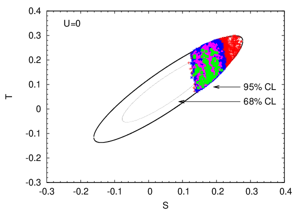
We also take into account the constraints from the oblique parameters [21]. In order to suppress the $S$-parameter, $M_{t^{\prime}}>M_{b^{\prime}}$ and/or $M_{\tau^{\prime}}>M_{\nu^{\prime}}$ are favorable. Although it increases the $T$-parameter, this is rather nice, because a relatively heavy Higgs pulls down $T$ [3, 5]. As for estimate of $S$ and $T$, we follow the LEP EWWG [25]. We obtain the central value as $(S,T)=(0.06,0.08)$, where the SM point is normalized to $(S,T)=(0,0)$ and the top mass $M_{t}=173.1$ GeV and the reference Higgs mass $M_{{\phi^{0}},ref}=117$ GeV are used. The relevant experimental values in the estimate are $M_{Z}=91.1875\pm 0.0021$ GeV, $\Delta\alpha_{{\rm had}}^{(5)}=0.02758\pm 0.00035$, $M_{W}=80.399\pm 0.0025$ GeV, $\sin^{2}\theta_{{\rm eff}}=0.23153\pm 0.00016$, and $\Gamma_{\ell}=83.985\pm 0.086$ MeV [26].

In Fig. 1, we depict scatter plots $M_{t^{\prime}}$ v.s. $M_{\phi^{0}}$ and $M_{\nu^{\prime}}$ v.s. $M_{\phi^{0}}$ within the 95% C.L. limit of the $(S,T)$-constraint. In each point, the fermion masses are different. We also showed the $(S,T)$-contour and the data points in the inset of the left of Fig. 1. For consistency of the model, the cutoff scale should not be so small. In the figure, we took the cutoff $\Lambda\geq 2$ TeV.

We find that the theoretical lower bound of the Higgs mass is $M_{\phi^{0}}\gtrsim M_{t^{\prime}}$, when $\Lambda\geq 2$ TeV. (If we take $\Lambda\geq 1$ TeV, slightly lower values of $M_{\phi^{0}}$ are allowed, $M_{\phi^{0}}\gtrsim M_{t^{\prime}}-\mbox{50 GeV}$.) Note that the Higgs production via the gluon fusion process is considerably enhanced owing to the loop effects of $t^{\prime}$ and $b^{\prime}$. For example, the cross section $\sigma_{gg\to\phi^{0}}$ for $M_{t^{\prime}}=M_{b^{\prime}}=0.4$ TeV and $M_{\phi^{0}}=0.5$ TeV increases by a factor of 5. Depending on the masses of $t^{\prime},b^{\prime}$ and $\phi^{0}$, the enhancement factor varies from 5 to 9. Consequently, a wider mass range of $M_{\phi^{0}}$ should be excluded at Tevatron. This potentially excluded mass range is fairly lower than the above Higgs mass bound, however [27].

In addition, the right of Fig. 1 clearly shows that the decay channel $\phi^{0}\to\bar{\nu}^{\prime}\nu^{\prime}$ is opened in a favorable parameter space. The importance of this process has been emphasized in Ref. [5], i.e., the new signal via $\phi^{0}\to\bar{\nu}^{\prime}\nu^{\prime}\to 4\ell+E\!\!\!/$, where $E\!\!\!/$ is the missing energy, can be comparable to the rate for $\phi^{0}\to ZZ\to 4\ell$. Moreover, we find that there is a parameter region where $\phi^{0}\to\bar{\tau}^{\prime}\tau^{\prime}$ is also kinematically allowed. In fact, several scenarios are possible. We show data samples in Table 1.

The constraints from the oblique parameters cause strong correlations between $M_{t^{\prime}}$ and $M_{b^{\prime}}$ and also between $M_{\tau^{\prime}}$ and $M_{\nu^{\prime}}$, as shown in the upper left and right of Fig. 2. The lower left of Fig. 2 suggests that there is no correlation between $M_{t^{\prime}}$ and $M_{\tau^{\prime}}$, as expected. On the other hand, the fermion mass differences are strongly correlated, as shown in the lower right of Fig. 2. This essentially corresponds to the constraint of the $T$-parameter,

We depicted it with $M_{\phi^{0}}=300\mbox{ GeV},\;500\mbox{ GeV}$ and $M_{{\phi^{0}},ref}=117$ GeV in the semicircles of the lower right of Fig. 2. The $S$-parameter constraint also suggests that the parameter region $M_{\tau^{\prime}}>M_{\nu^{\prime}}$ and $M_{t^{\prime}}>M_{b^{\prime}}$ is favorable. (Within the 95% C.L. limit, $M_{t^{\prime}}<M_{b^{\prime}}$ is also possible with paying cost of a worse $\chi^{2}$, as shown in the lower right of Fig. 2. )

We emphasize that in a wide parameter region, we find $M_{\tau^{\prime}}>M_{\nu^{\prime}}+M_{W}$, i.e., the decay channel $\tau^{\prime}\to\nu^{\prime}+W^{-}$ is allowed. (The situation is unchanged, even if we take $\Lambda\geq 1$ TeV.) Also, $t^{\prime}\to b^{\prime}+W^{(*)}$ is possible. These do not necessarily contradict the results in Ref. [5]: Since the Higgs is inevitably heavy in our approach, the $T$-parameter constraint requires a larger mass difference of the fermions than that of Ref. [5]. (The $\chi^{2}$ is a bit worse, however.)

The implications of Figs. 1–2 are obvious: If $t^{\prime}$ and/or $b^{\prime}$ are discovered at the Tevatron and/or LHC, the Higgs mass will be suggested under the assumption of the SM4. On the other hand, if the LHC excludes $M_{t^{\prime},b^{\prime}}\lesssim 500$ GeV, only few points survive when we take $\Lambda\geq 2$ TeV. I.e., a model with the cutoff $\Lambda<2$ TeV or a nonperturbative regime will be left to be explored.

We have reanalyzed the constraints on the mass spectrum of the fourth generation fermions and the Higgs bosons for the SM4 and the THDM II with $\sin(\beta-\alpha)=1$. We showed that there are the noticeable correlations among the mass spectrum of the fermions and the Higgs bosons.

For the SM4, the favorable mass range of the physical Higgs boson $\phi^{0}$ is $M_{\phi^{0}}\gtrsim M_{t^{\prime}}$ ($M_{\phi^{0}}\gtrsim M_{t^{\prime}}-\mbox{50 GeV}$) for the cutoff $\Lambda\geq 2$ TeV ($\Lambda\geq 1$ TeV). We also found that the favorable parameter space is mainly contained in the region,

and

(See also the semicircles in lower right of Fig. 2.) We showed the data samples corresponding to several scenarios in Table 1.

For the THDM II with $\sin(\beta-\alpha)=1$, schematically speaking, there are two domains for the favorable mass range of the light CP even Higgs $h$, $M_{h}\gtrsim M_{t^{\prime}}$ and $M_{h}\lesssim M_{t^{\prime}}$. The extra heavy Higgs decoupling regime is contained in the former. This is consistent with the analysis of the SM4. On the other hand, an almost degenerate Higgs mass spectrum such as $M_{h}\approx\mbox{100--300 GeV}$ and $M_{H}\sim M_{H^{\pm}}\sim M_{A}\sim\mbox{300--400 GeV}$ is allowed in the latter and in a part of the former. In this case, a model with $M^{2}=0$ is not excluded. (See the right of Fig. 7.) As for the value of $\tan\beta$, we found that $\tan\beta\approx 1$ is favorable in the both domains.

Concerning the decay channels of the charged leptons, we found that $\tau^{\prime}\to\nu^{\prime}+W^{-}$ is allowed in a wide parameter space in the SM4 and the THDM II. (See the lower right of Figs. 2 and 5.) The fourth generation quark masses can be degenerate $M_{t^{\prime}}=M_{b^{\prime}}$ or the decay channel $t^{\prime}\to b^{\prime}+W^{(*)}$ can be open, depending on the mass difference $M_{\tau^{\prime}}-M_{\nu^{\prime}}$. (See the lower right of Figs. 2 and 5.) The Higgs $\phi^{0}$ in the SM4 and the light CP even Higgs $h$ in the THDM II can decay into a pair of the fourth generation neutrinos. (See the right of Figs. 1 and 3.) Furthermore, in the THDM II, a scenario that all Higgs bosons decay into a pair of the fourth generation leptons is possible, i.e., $h\to\bar{\nu}^{\prime}\nu^{\prime}$ and $H^{-}\to\bar{\nu}^{\prime}\tau^{\prime}$, etc.. (For studies of collider signals of the fourth generation leptons, see, e.g., Ref. [40].) We also comment that the main decay channel of the heavy CP even Higgs $H$ can be $H\to\bar{t}^{\prime}t^{\prime},\bar{b}^{\prime}b^{\prime}$, if kinematically allowed [41]. Thus the phenomenology of the fourth generation models is very rich.

References

- [1] For a comprehensive review, see, e.g., P. H. Frampton, P. Q. Hung and M. Sher, Phys. Rept. 330, 263 (2000).
- [2] For a recent overview, see, e.g., B. Holdom, W. S. Hou, T. Hurth, M. L. Mangano, S. Sultansoy and G. Unel, PMC Phys. A 3, 4 (2009) [arXiv:0904.4698 [hep-ph]].
- [3] H. J. He, N. Polonsky and S. f. Su, Phys. Rev. D 64, 053004 (2001).
- [4] V. A. Novikov, L. B. Okun, A. N. Rozanov and M. I. Vysotsky, JETP Lett. 76, 127 (2002) [Pisma Zh. Eksp. Teor. Fiz. 76, 158 (2002)] [arXiv:hep-ph/0203132]; V. A. Novikov, A. N. Rozanov and M. I. Vysotsky, arXiv:0904.4570 [hep-ph].
- [5] G. D. Kribs, T. Plehn, M. Spannowsky and T. M. P. Tait, Phys. Rev. D 76, 075016 (2007) [arXiv:0706.3718 [hep-ph]].
- [6] J. A. Aguilar-Saavedra, Phys. Lett. B 625, 234 (2005) [Erratum-ibid. B 633, 792 (2006)]; O. Cakir, H. Duran Yildiz, R. Mehdiyev and I. Turk Cakir, Eur. Phys. J. C 56, 537 (2008) [arXiv:0801.0236 [hep-ph]]; V. E. Ozcan, S. Sultansoy and G. Unel, arXiv:0802.2621 [hep-ex]; V. E. Ozcan, S. Sultansoy and G. Unel, Eur. Phys. J. C 57 (2008) 621; E. L. Berger and Q. H. Cao, arXiv:0909.3555 [hep-ph].
- [7] B. Holdom, Phys. Rev. Lett. 57, 2496 (1986) [Erratum-ibid. 58, 177 (1987)]; C. T. Hill, M. A. Luty and E. A. Paschos, Phys. Rev. D 43, 3011 (1991); B. Holdom, Phys. Rev. D 54, 721 (1996); JHEP 0608, 076 (2006).
- [8] M. Hashimoto and V. A. Miransky, Phys. Rev. D 80, 013004 (2009) [arXiv:0901.4354 [hep-ph]].
- [9] M. Hashimoto and V. A. Miransky, arXiv:0912.4453 [hep-ph].
- [10] For a comprehensive review, see, J. F. Gunion, H. E. Haber, G. Kane,and S. Dawson, The Higgs Hunter’s Guide (Perseus Publishing, Cambridge, MA, 1990).
- [11] See, e.g., J. F. Gunion and H. E. Haber, Phys. Rev. D 67, 075019 (2003).
- [12] C. T. Hill, Phys. Lett. B 266, 419 (1991); C. T. Hill, Phys. Lett. B 345, 483 (1995); For a recent comprehensive review, see, e.g., C. T. Hill and E. H. Simmons, Phys. Rept. 381, 235 (2003) [Erratum-ibid. 390, 553 (2004)].
- [13] W. A. Bardeen, C. T. Hill and M. Lindner, Phys. Rev. D 41, 1647 (1990).
- [14] M. A. Luty, Phys. Rev. D 41, 2893 (1990).
- [15] N. G. Deshpande and E. Ma, Phys. Rev. D 18, 2574 (1978).
- [16] For a review, see, M. Sher, Phys. Rept. 179, 273 (1989).
- [17] M. S. Chanowitz, M. A. Furman and I. Hinchliffe, Phys. Lett. B 78, 285 (1978); Nucl. Phys. B 153, 402 (1979).
- [18] B. W. Lee, C. Quigg and H. B. Thacker, Phys. Rev. Lett. 38, 883 (1977); Phys. Rev. D 16, 1519 (1977).
- [19] S. Kanemura, T. Kubota and E. Takasugi, Phys. Lett. B 313, 155 (1993) [arXiv:hep-ph/9303263].
- [20] A. G. Akeroyd, A. Arhrib and E. M. Naimi, Phys. Lett. B 490, 119 (2000) [arXiv:hep-ph/0006035].
- [21] M. E. Peskin and T. Takeuchi, Phys. Rev. Lett. 65, 964 (1990); Phys. Rev. D 46, 381 (1992).
- [22] For a general discussion including the two-loop effects, see, e.g., M. E. Machacek and M. T. Vaughn, Nucl. Phys. B 222, 83 (1983); Nucl. Phys. B 236, 221 (1984); Nucl. Phys. B 249, 70 (1985).
- [23] There has been numerous works on this subject, for example, C. T. Hill, Phys. Rev. D 24, 691 (1981); C. Wetterich, Phys. Lett. B 104, 269 (1981); M. Tanimoto, T. Hayashi, R. Najima and S. Wakaizumi, Prog. Theor. Phys. 76, 1098 (1986); H. B. Nielsen, A. V. Novikov, V. A. Novikov and M. I. Vysotsky, Phys. Lett. B 374, 127 (1996) [arXiv:hep-ph/9511340]; D. Dooling, K. Kang and S. K. Kang, Int. J. Mod. Phys. A 14, 1605 (1999) [arXiv:hep-ph/9710258]; P. Q. Hung, Phys. Rev. Lett. 80, 3000 (1998) [arXiv:hep-ph/9712338]; Yu. F. Pirogov and O. V. Zenin, Eur. Phys. J. C 10, 629 (1999) [arXiv:hep-ph/9808396].
- [24] C. Amsler et al. [Particle Data Group], Phys. Lett. B 667, 1 (2008).
- [25] [ALEPH Collaboration and DELPHI Collaboration and L3 Collaboration and ], Phys. Rept. 427, 257 (2006) [arXiv:hep-ex/0509008].
- [26] [ALEPH Collaboration and CDF Collaboration and D0 Collaboration and an], arXiv:0811.4682 [hep-ex]; http://lepewwg.web.cern.ch/LEPEWWG/
- [27] N. B. Schmidt, S. A. Cetin, S. Istin and S. Sultansoy, arXiv:0908.2653 [hep-ph].
- [28] A. Lister [CDF Collaboration], arXiv:0810.3349 [hep-ex]; T. Aaltonen et al. [The CDF Collaboration], arXiv:0912.1057 [hep-ex].
- [29] S. L. Glashow and S. Weinberg, Phys. Rev. D 15, 1958 (1977).
- [30] For the analysis in the three generation model, see, e.g., S. Nie and M. Sher, Phys. Lett. B 449, 89 (1999) [arXiv:hep-ph/9811234]; S. Kanemura, T. Kasai and Y. Okada, Phys. Lett. B 471, 182 (1999) [arXiv:hep-ph/9903289].
- [31] C. T. Hill, C. N. Leung and S. Rao, Nucl. Phys. B 262, 517 (1985).
- [32] S. Kanemura, Y. Okada, E. Senaha and C. P. Yuan, Phys. Rev. D 70, 115002 (2004) [arXiv:hep-ph/0408364].
- [33] See, e.g., K. Cheung and O. C. W. Kong, Phys. Rev. D 68, 053003 (2003); A. Wahab El Kaffas, P. Osland and O. M. Ogreid, Phys. Rev. D 76, 095001 (2007).
- [34] M. Misiak et al., Phys. Rev. Lett. 98, 022002 (2007) [arXiv:hep-ph/0609232].
- [35] O. Deschamps, S. Descotes-Genon, S. Monteil, V. Niess, S. T’Jampens and V. Tisserand, arXiv:0907.5135 [hep-ph].
- [36] A. Denner, R. J. Guth, W. Hollik and J. H. Kuhn, Z. Phys. C 51, 695 (1991).
- [37] H. E. Haber and H. E. Logan, Phys. Rev. D 62, 015011 (2000) [arXiv:hep-ph/9909335].
- [38] R. Barate et al. [LEP Working Group for Higgs boson searches and ALEPH Collaboration], Phys. Lett. B 565, 61 (2003) [arXiv:hep-ex/0306033].
- [39] H. Komatsu, Prog. Theor. Phys. 67, 1177 (1982).
- [40] T. Cuhadar-Donszelmann, M. K. Unel, V. E. Ozcan, S. Sultansoy and G. Unel, JHEP 0810, 074 (2008) [arXiv:0806.4003 [hep-ph]]; V. E. Ozcan, S. Sultansoy and G. Unel, J. Phys. G 36, 095002 (2009) [arXiv:0903.3177 [hep-ex]].
- [41] S. Bar-Shalom, G. Eilam and A. Soni, arXiv:1001.0569 [hep-ph].
- [42] V. D. Barger, J. L. Hewett and R. J. N. Phillips, Phys. Rev. D 41, 3421 (1990); Y. Grossman, Nucl. Phys. B 426, 355 (1994) [arXiv:hep-ph/9401311]; M. Aoki, S. Kanemura, K. Tsumura and K. Yagyu, Phys. Rev. D 80, 015017 (2009) [arXiv:0902.4665 [hep-ph]]; S. Su and B. Thomas, Phys. Rev. D 79, 095014 (2009) [arXiv:0903.0667 [hep-ph]]; H. E. Logan and D. MacLennan, Phys. Rev. D 79, 115022 (2009) [arXiv:0903.2246 [hep-ph]].
- [43] S. Bertolini and A. Sirlin, Phys. Lett. B 257, 179 (1991); E. Gates and J. Terning, Phys. Rev. Lett. 67, 1840 (1991); B. A. Kniehl and H. G. Kohrs, Phys. Rev. D 48, 225 (1993); see also the last two of Ref. [7].
- [44] M. Bobrowski, A. Lenz, J. Riedl and J. Rohrwild, Phys. Rev. D 79, 113006 (2009) [arXiv:0902.4883 [hep-ph]].
- [45] M. S. Chanowitz, Phys. Rev. D 79, 113008 (2009) [arXiv:0904.3570 [hep-ph]].
- [46] S. Kanemura, S. Kiyoura, Y. Okada, E. Senaha and C. P. Yuan, Phys. Lett. B 558, 157 (2003) [arXiv:hep-ph/0211308].
- [47] U. Baur, T. Plehn and D. L. Rainwater, Phys. Rev. Lett. 89, 151801 (2002); Phys. Rev. D 67, 033003 (2003); see also, F. Gianotti et al., Eur. Phys. J. C 39, 293 (2005).
- [48] V. A. Ilyin, A. E. Pukhov, Y. Kurihara, Y. Shimizu and T. Kaneko, Phys. Rev. D 54, 6717 (1996) [arXiv:hep-ph/9506326]; G. Belanger et al., Phys. Lett. B 576, 152 (2003) [arXiv:hep-ph/0309010]; E. Asakawa, D. Harada, S. Kanemura, Y. Okada and K. Tsumura, Phys. Lett. B 672, 354 (2009) [arXiv:0809.0094 [hep-ph]].
- [49] W. S. Hou, M. Nagashima, G. Raz and A. Soddu, JHEP 0609, 012 (2006) [arXiv:hep-ph/0603097]; W. S. Hou, M. Nagashima and A. Soddu, Phys. Rev. Lett. 95, 141601 (2005) [arXiv:hep-ph/0503072]; W. S. Hou, H. n. Li, S. Mishima and M. Nagashima, Phys. Rev. Lett. 98, 131801 (2007) [arXiv:hep-ph/0611107]; W. S. Hou, M. Nagashima and A. Soddu, Phys. Rev. D 76, 016004 (2007) [arXiv:hep-ph/0610385].
- [50] A. Soni, A. K. Alok, A. Giri, R. Mohanta and S. Nandi, arXiv:0807.1971 [hep-ph].
- [51] M. S. Carena, A. Megevand, M. Quiros and C. E. M. Wagner, Nucl. Phys. B 716, 319 (2005) [arXiv:hep-ph/0410352]; Y. Kikukawa, M. Kohda and J. Yasuda, Prog. Theor. Phys. 122, 401 (2009) [arXiv:0901.1962 [hep-ph]].
- [52] M. S. Chanowitz, Phys. Rev. Lett. 69, 2037 (1992); Phys. Lett. B 352, 376 (1995) [arXiv:hep-ph/9503458].