Large Fluctuations of the Macroscopic Current in Diffusive Systems:
A Confirmation of the Additivity Principle
Abstract
Most systems, when pushed out of equilibrium, respond by building up currents of locally-conserved observables. Understanding how microscopic dynamics determines the averages and fluctuations of these currents is one of the main open problems in nonequilibrium statistical physics. The additivity principle is a theoretical proposal that allows to compute the current distribution in many one-dimensional nonequilibrium systems. Using simulations, we confirm this conjecture in a simple and general model of energy transport, both in the presence of a temperature gradient and in canonical equilibrium. In particular, we show that the current distribution displays a Gaussian regime for small current fluctuations, as prescribed by the central limit theorem, and non-Gaussian (exponential) tails for large current deviations, obeying in all cases the Gallavotti-Cohen fluctuation theorem. In order to facilitate a given current fluctuation, the system adopts a well-defined temperature profile different from that of the steady state, and in accordance with the additivity hypothesis predictions. System statistics during a large current fluctuation is independent of the sign of the current, which implies that the optimal profile (as well as higher-order profiles and spatial correlations) are invariant upon currenst inversion. We also demonstrate that finite-time joint fluctuations of the current and the profile are well described by the additivity functional. These results confirm the additivity hypothesis as a general and powerful tool to compute current distributions in many nonequilibrium systems.
I Introduction
Understanding the physics of systems out of equilibrium remains challenging to a large extent, even in the simplest setting for which one could expect to make significant advances, which is that of a nonequilibrium steady state (NESS). Even in this simple situation difficulties abound mainly because out of equilibrium the dynamics plays a dominant role [1, 2]. For instance, the phase space available to a system in a NESS depends crucially on the dynamics, resulting in a probability measure for microscopic configurations which is not known in general for a NESS, as it will inherit this dependence on the dynamics [3]. This is in contrast to the equilibrium case, where the available phase space is uniquely determined by the Hamiltonian and the Gibss distribution provides the probability measure for microscopic configurations. One can ask however questions on the statistics of the macroscopic observables characterizing a NESS, as for instance the current flowing through the system [4, 5, 6, 7]. In equilibrium, the fluctuations of macroscopic quantities, which are a reflection of the hectic microscopic world, are strikingly independent of microscopic details, being solely determined by thermodynamic quantities as the entropy, free energy, etc. A natural way to seek a macroscopic theory of nonequilibrium phenomena is thus to investigate the fluctuations of macroscopic currents. Unveiling the relation between microscopic dynamics and current fluctuations has proven to be a difficult task [4, 5, 6, 7, 8, 9, 10, 11, 12, 13], and up to now only few exactly-solvable cases are understood. An important step in this direction has been the development of the Gallavotti-Cohen fluctuation theorem [12, 13], which relates the probability of forward and backward currents reflecting the time-reversal symmetry of microscopic dynamics. However, we still lack a general approach based on few simple principles. Recently, Bertini, De Sole, Gabrielli, Jona-Lasinio and Landim [4] have introduced a Hydrodynamic Fluctuation Theory (HFT) to study large dynamic fluctuations of diffusive systems. This is a very general approach which leads to a hard variational problem whose solution remains challenging in most cases. Simultaneously, Bodineau and Derrida [5, 6, 7] have conjectured an additivity principle for current fluctuations in one dimension which can be readily applied to obtain quantitative predictions and, together with HFT, seems to open the door to a general theory for nonequilibrium systems.
In this paper we test in depth the validity of the additivity principle in a simple and very general diffusive model. In particular, we investigate the fluctuations of the energy current in the one-dimensional (1D) Kipnis-Marchioro-Pressuti (KMP) model of heat conduction, which represents at a coarse-grained level a large class of quasi-1D diffusive systems of technological and theoretical interest for which understanding current statistics is of central importance. Our results strongly support the validity of the additivity principle to describe current fluctuations in one dimension, both in the presence of a temperature gradient (NESS) and in canonical equilibrium. In particular, we find that the current distribution shows both Gaussian and non-Gaussian regimes, and obeys the Gallavotti-Cohen symmetry. The system modifies its temperature profile to facilitate a given current fluctuation, as predicted by the theory, and this profile (as well as any other higher-order profile and spatial correlation) turns out to be independent of the sign of the current. We also explore physics beyond the additivity conjecture by studying the fluctuations of the total energy in the system, which exhibit the trace left by corrections to local equilibrium resulting from the presence of weak long-range correlations in the NESS. In addition, we extend the additivity hypothesis to study the joint fluctuations of the current and the profile.
The paper is structured as follows. In next section we describe the additivity principle from a general perspective. Section III introduces the KMP model in one dimension. In section IV we report the results of our simulations, together with a detailed comparison with theoretical predictions. Here we also show evidence of structure beyond the additivity scenario. Section V investigates the joint fluctuations of the current and the temperature profile, extending the additivity principle to understand these finite-time corrections. Finally, we present our conclusions in section VI, and a number of appendices describe some technical aspects of the discussion in the main text. Part of the work reported in this paper was presented in a shorter Letter [14].
II The Additivity Principle
The additivity principle (to which we will also refer here as BD theory) is a conjecture first proposed by T. Bodineau and B. Derrida [5] that enables one to calculate the fluctuations of the current in 1D diffusive systems in contact with two boundary thermal baths at different temperatures, . It is a very general conjecture of broad applicability, expected to hold for 1D systems of classical interacting particles, both deterministic or stochastic, independently of the details of the interactions between the particles or the coupling to the thermal reservoirs. The only requirement is that the system at hand must be diffusive, i.e. Fourier’s law must hold. If this is the case, the additivity principle predicts the full current distribution in terms of its first two cumulants. Equivalently, one may use the same formalism to study diffusive particle systems coupled to particle reservoirs at the boundaries at different chemical potentials, and obeying Fick’s law, or any other open diffusive system characterized by a single locally-conserved field. However, in this paper we stick for simplicity to the energy-diffusion version of the problem. Let be the probability of observing a time-integrated current during a long time in a system of size . This probability typically obeys a large deviation principle [15, 16],
| (1) |
where is the current large-deviation function (LDF), such that and , with . This means in particular that current fluctuations away from the average are exponentially unlikely in time. The additivity principle relates this probability with the product of probabilities for sustaining the same current in subsystems of lengths and ,
| (2) |
The maximization over the contact temperature can be rationalized by writing the above probability as an integral over of the product of probabilities for subsystems and noticing that these should obey also a large deviation principle akin to eq. (1). Hence a saddle-point calculation in the long- limit leads to (2). The additivity principle can be then rewritten for the large deviation function as
| (3) |
We now may adopt a scaling form for the current LDF [5, 6, 7], and proceed by slicing iteratively the 1D system of length into smaller and smaller segments. For small enough segments the temperature difference across each of them will be small, so for small currents each interval can be considered to be close to equilibrium and hence exhibits locally-Gaussian fluctuations around the average current (given by Fourier’s law) at the leading order. In this way we obtain in the continuum limit the following variational form for [5, 6, 7]
| (4) |
where we dropped the dependence on the baths for convenience. Here is the thermal conductivity characterizing Fourier’s law, , and measures current fluctuations in equilibrium (), . The optimal temperature profile derived from (4) by functional differentiation obeys
| (5) |
where is a constant which guarantees the correct boundary conditions, and . In what follows we assume without loss of generality. Equations (4) and (5) completely determine the current distribution, which is in general non-Gaussian (except for very small current fluctuations) and obeys the Gallavotti-Cohen symmetry,
| (6) |
with a constant defined by [5]
Moreover, the optimal profile solution of eq. (5) is independent of the sign of the current, , a rather counter-intuitive result which, together with the Gallavotti-Cohen relation, reflects the time-reversal symmetry of microscopic dynamics [12, 13].
In the simplest case, when is large enough for the rhs of eq. (5) not to vanish –something that happens for currents close to the average, the optimal profile is monotone and we have ()
| (7) |
Using this expression in eq. (4) leads to
| (8) |
and integrating eq. (7) above over the whole interval we obtain an implicit equation for ,
| (9) |
In many applications it is interesting to work with the Legendre transform of the large deviation function,
| (10) |
or equivalently , with given by . By noticing that , it then follows for monotone profiles
| (11) |
where is now obtained from
| (12) |
and is the sign function. The function can be viewed as the conjugate potential to , with the parameter conjugate to the current , a relation equivalent to the free energy being the Legendre transform of the internal energy in thermodynamics, with the temperature as conjugate parameter to the entropy.
When the constant is negative enough for the rhs of eq. (5) to vanish at some point, the resulting optimal profile becomes non-monotone. In this case it can be shown [5] that the expressions for and , or their equivalent formulas in -space, are just the analytic continuation of their monotone-case counterparts. Appendix A shows the particular expressions for the current LDF and the associated optimal profile, both in the monotone and non-monotonous cases, as derived when applying this general scheme to the particular model of interest in this paper, the Kipnis-Marchioro-Presutti (KMP) model of heat conduction [17].
Before continuing with the description of this model, it is worth noticing that the additivity principle can be better understood within the context of Hydrodynamic Fluctuation Theory of Bertini et al. [4], which provides a variational principle for the most probable (possibly time-dependent) profile responsible of a given current fluctuation. The probability of observing a particular history of the temperature profile and the rescaled current during a macroscopic time is, according to HFT [4, 18],
| (13) |
where the functional can be written as
| (14) |
and where the rescaled current field is related to the temperature profile via the continuity equation . The large deviation function of the integrated current is then
| (15) |
where is related to via
| (16) |
with the constraint
| (17) |
and and coupled via the above continuity equation. Solving this time-dependent problem to obtain explicit predictions for the current LDF remains a challenge in most cases. The additivity principle, which on the other hand can be readily applied to obtain quantitative predictions, is equivalent within HFT to the hypothesis that the optimal profiles and solution of the variational problem (16)-(17) are time-independent, in which case we recover eq. (4) for . In some special cases this approximation breaks down for for extreme current fluctuations [4, 18, 19], but even so the additivity hypothesis correctly predicts the current LDF in a very large current interval, making it very appealing.
III The KMP Model

The system is defined on a 1D open lattice with sites [17]. Each site models an harmonic oscillator which is mechanically uncoupled from its nearest neighbors but interact with them through a random process which redistributes energy locally. In this way, a configuration is given by , where is the energy of site , and the stochastic dynamics proceeds through random energy exchanges between randomly-chosen nearest neighbors, i.e. for such that
| (18) |
with a homogeneous random number so . In addition, boundary sites () may also exchange energy with boundary heat baths at temperatures for and for , i.e. such that
| (19) |
with randomly drawn at each step from a Gibbs distribution at the corresponding temperature, , , and random. For KMP proved [17] that the system reaches a nonequilibrium steady state which, in the hydrodynamic scaling limit, is described by Fourier’s law with a nonzero average current
| (20) |
with , and a linear energy profile
| (21) |
In addition, convergence to the local Gibbs measure was proven in this limit [17], meaning that , , has an exponential distribution with local temperature in the thermodynamic limit. However, corrections to Local Equilibrium (LE), though vanishing in the limit, become apparent at the fluctuation level [26, 27], as we will show below. Moreover, the fluctuations of the current in equilibrium () are described by . It is also worth noticing that KMP dynamics obeys the local detailed balance condition and is therefore time-reversible [13], see Appendix D. In this way we expect the Gallavotti-Cohen symmetry to hold in this system, see eq. (6).

The KMP model plays a fundamental role in nonequilibrium statistical physics as a benchmark to test new theoretical advances, and represents at a coarse-grained level a large class of quasi-1D diffusive systems of technological and theoretical interest. In this way, understanding how the energy current fluctuates in the KMP model is of central importance to understand current statistics in more realistic systems. Furthermore, the KMP model is an optimal candidate to test the additivity principle because: (i) One can solve eqs. (4) and (5) to obtain explicit predictions for its current LDF, and (ii) its simple dynamical rules allow a detailed numerical study of current fluctuations.
In Appendix A we apply the additivity formalisms of the previous section to study current fluctuations in the KMP model. In particular, we use eqs. (4) and (5) to derive analytical expressions for the current LDF and the associated optimal profiles , see Figs. 1-2. In this case it can be shown that optimal profiles can be either monotone or non-monotone with a single maximum, see Appendix A for the explicit calculations. In what follows, we compare this set of analytical predictions with computer simulation results.
IV Numerical Test of the Additivity Principle


The simplicity and versatility of the KMP model allows us to obtain explicit analytical expressions for and based on the additivity conjecture, see Appendix A. Figs. 1 and 2 show the theoretical current LDF and the associated optimal profiles, respectively. We find that is Gaussian around with variance , while non-Gaussian, exponential tails develop far from , with decay rates given by the inverse bath temperatures. Exploring by standard simulations these tails to check BD theory is very difficult, since LDFs involve by definition exponentially-unlikely rare events. This is corroborated in Appendix B, where is measured directly but we are unable to gather enough statistics in the tails of the current distribution to validate or falsify the additivity hypothesis. Recently Giardinà, Kurchan and Peliti [20] have introduced an efficient method to measure LDFs in many particle systems, based on a modification of the dynamics so that the rare events responsible of the large deviation are no longer rare [21]. This method yields the Legendre transform of the current LDF, , see eq. (10), If is the transition rate from configuration to of the associated stochastic process, the modified dynamics is defined as , where is the elementary current involved in the transition . It can be then shown (see Appendix C) that the natural logarithm of the largest eigenvalue of matrix gives . The method of Ref. [20] thus provides a way to measure by evolving many copies or clones of the system using the modified dynamics , see Appendix C.
We applied the method of Giardinà et al. to measure for the 1D KMP model with , and , see Fig. 3, top panel. The agreement with BD theory is excellent for a wide -interval, say , which corresponds to a very large range of current fluctuations, see inset to Fig. 11 in Appendix C. Moreover, the deviations observed for extreme current fluctuations are due to known limitations of the algorithm [14, 20, 21, 22], so no violations of additivity are observed. Notice that the spurious differences seem to occur earlier for currents against the gradient, i.e. . In fact, we can use the Gallavotti-Cohen symmetry, which in -space now reads with , to bound the range of validity of the algorithm: Violations of the fluctuation relation indicate a systematic bias in the estimations provided by the method of Ref. [20], see also [22]. Fig. 4. shows that the Gallavotti-Cohen symmetry holds in the large current interval for which the additivity principle predictions agree with measurements, thus confirming its validity in this range. However, we cannot discard the possibility of an additivity breakdown for extreme current fluctuations due to the onset of time-dependent optimal profiles expected in general in HFT [4], although we stress that such scenario is not observed here.
We also measured the current LDF in canonical equilibrium, i.e. for , see the bottom panel in Fig. 3. The agreement with BD theory is again excellent within the range of validity of our measurements, which expands a wide current interval, see inset to Fig. 3, and the fluctuation relation is verified except for extreme currents deviations, where the algorithm fails to provide reliable results. Notice that, both in the presence of a temperature gradient and in canonical equilibrium, is parabolic around meaning that current fluctuations are Gaussian for , as demanded by the central limit theorem, see eqs. (60)-(61) in Appendix A. This observation is particularly interesting in equilibrium, where canonical and microcanonical ensembles behave differently (see below).


The additivity principle leads to the minimization of a functional of the temperature profile, , see eqs. (4) and (5). A relevant question is whether this optimal profile is actually observable. We naturally define as the average energy profile adopted by the system during a large deviation event of (long) duration and time-integrated current , measured at an intermediate time , i.e. . Fig. 5 shows the measured for both the equilibrium and nonequilibrium settings, and the agreement with BD predictions is again very good in all cases, with discrepancies appearing only for extreme current fluctuations, as otherwise expected. See also Fig. 14 in Appendix B. This confirms the idea that the system indeed modifies its temperature profile to facilitate the deviation of the current, validating the additivity principle as a powerful conjecture to compute both the current LDF and the associated optimal profiles. Our numerical results show also that optimal profiles are indeed independent of the sign of the current, or equivalently , a counter-intuitive symmetry resulting from the reversibility of microscopic dynamics. Notice that in the equilibrium case () optimal temperature profiles are always non-monotone with a single maximum for any current fluctuation (the stationary profile is obviously flat). This is in stark contrast to the behavior predicted for current fluctuations in microcanonical equilibrium, i.e. for a one-dimensional closed diffusive system on a ring [4, 18, 19]. In this case the optimal profiles remain flat and current fluctuations are Gaussian up to a critical current value, at which profiles become time-dependent (traveling waves) [19]. Hence current statistics can differ considerably depending on the particular equilibrium ensemble at hand, despite their equivalence for average quantities in the thermodynamic limit. Finally, notice also that equilibrium optimal profiles are symmetric with respect to , as expected since .

For small enough current fluctuations around the average, with for and , BD theory predicts the limiting behavior
| (22) |
Fig. 6 confirms this scaling for and many different small current fluctuations around the average. In particular, it shows data obtained both from standard simulations (see Appendix B) and using the advanced method of Ref. [20].
It is also interesting to study the statistics of configurations both during a large deviation event and at the end. They differ due to final transient effects which decay exponentially fast, but a connection exists between both regimes which highlights the symmetry of midtime statistics resulting from the reversibility of microscopic dynamics (a symmetry akin to the fluctuation relation). Reversibility in stochastic dynamics stems from the condition of local detailed balance [13], which implies a relation between the forward modified dynamics for a current fluctuation, , and the time-reversed modified dynamics for the negative fluctuation, , see eq. (90) in Appendix D. This can be used to derive a relation between midtime and endtime statistics (see Appendix D),
| (23) |
Here [resp. ] is the probability of configuration at the end (resp. at intermediate times) of a large deviation event with current-conjugate parameter , and is an effective weight for configuration , with , while is a normalization constant. Eq. (23) implies that configurations with a significant contribution to the average profile at intermediate times are those with an important probabilistic weight at the end of both the large deviation event and its time-reversed process. An important consequence of eq. (23) is hence that , or equivalently , so midtime statistics does not depend on the sign of the current. This implies in particular that , but also that all higher-order profiles and spatial correlations are independent of the current sign .


The above connection allows us to relate midtime and endtime profiles for a given current fluctuation. For that we need additionally a local equilibrium (LE) hypothesis, i.e. we now assume that spatial correlations at the end of a large deviation event are weak enough so the distribution can be approximately factorized, . In this way we obtain a local equilibrium picture with local temperature parameter . This hypothesis can be numerically justified by measuring, at the end of the large deviation event, local energy distributions along the chain for different values of , see Fig. 7. In all cases the distribution is compatible with local equilibrium to a large degree of accuracy. Using eq. (23) and the LE hypothesis we thus find
| (24) |
Fig. 8 shows endtime profiles measured both in equilibrium (bottom) and nonequilibrium (top) conditions for different values of . These profiles are clearly asymmetric upon current inversion, , and most interestingly they show boundary resistance which depends on and on the particular definition for the elementary current, see [22]. In the equilibrium case the symmetry resulting from the reflection invariance in this case () is apparent in Fig. 8 (bottom). Fig. 5 also shows midtime profiles obtained from the measured via eq. (24). The agreement with theoretical predictions and direct measurements of midtime profiles is good, though discrepancies appear for large enough current fluctuations, pointing out that corrections to LE are weak but increase for large current deviations. We show below that these corrections are also present for small current fluctuations and can be measured.

We can now explore physics beyond the additivity conjecture by studying fluctuations of the system total energy, , for which current theoretical approaches cannot offer any general prediction. An exact result by Bertini, Gabrielli and Lebowitz (BGL) [27] predicts that
| (25) |
where is the variance of the total energy in the nonequilibrium steady state (NESS), is the variance assuming a local equilibrium (LE) product measure, and the last term reflects the correction to LE due to weak long-range correlations in the NESS [27], which in this case results in the enhancement of energy fluctuations. Corrections to LE vanish in the thermodynamic limit but extend over macroscopic distances (of order ), giving rise in general to a non-local current LDF [27]. In our case,
| (26) |
while . Fig. 9 plots as a function of for both equilibrium and nonequilibrium conditions, showing a non-trivial, interesting structure which both BD theory and HFT cannot explain. One might obtain a theoretical prediction for by supplementing the additivity principle with a LE hypothesis,
| (27) |
which results in
| (28) |
This prediction agrees qualitatively with the observed behavior, though fine quantitative differences are apparent, see Fig. 9, as otherwise expected. In particular we find that, out of equilibrium, as corresponds to a LE picture, and in contrast to the measured value in Fig. 9, which compares nicely with the exact BGL result (recall that corresponds to ). This shows that, even though LE is a sound numerical hypothesis to obtain from endtime statistics for small and moderate current fluctuations, see Fig. 5 and eq. (24), corrections to LE become apparent at the fluctuating level even for small current fluctuations. This is also shown in Fig. 15 in Appendix B, where fluctuations of the total energy under nonequilibrium conditions are studied in standard simulations. On the other hand, in the canonical equilibrium case () no corrections to LE show up for (i.e., for ), as expected. However, as soon as , deviations of from the LE prediction are observed, thus showing that local equilibrium is broken at the fluctuating level even for equal bath temperatures.
Finally, the inset to Fig. 9 shows the average energy per site as a function of , together with the prediction based on the additivity principle, . Agreement is again very good in the large range of currents explored. It is interesting to note that in order to sustain a current fluctuation above the average, or equivalently , the nonequilibrium system () has always a larger average energy than its equilibrium counterpart (), while the reverse holds for current fluctuations below the average, , see inset to Fig. 9.
V Joint Fluctuations of the Current and the Profile
For long but finite times, the profile associated to a given current fluctuation is subject to fluctuations itself. These joint fluctuations of the current and the profile are again not described by the additivity principle, but we may study them by extending the additivity conjecture. In this way, we now assume that the probability to find a time-integrated current and a temperature profile after averaging for a long but finite time can be written as
| (29) |
where now
| (30) |
Notice that here no minimization with respect to temperature profiles is performed, see eq. (4). In this scheme the profile obeying eq. (5), i.e. the one which minimizes the functional , is the classical profile . For a given value we can make a perturbation of around its classical value,
| (31) |
For large enough , the joint probability of and can be written as
| (32) |
where is defined in equation (1), together with eqs. (4) and (5). The integral kernel is
| (33) | |||||

One can show that the kernel is symmetric with respect to and . In order to check the above joint probability distribution, we studied the observable
| (34) |
where
| (35) |
and and are the eigenvectors and eigenvalues of kernel , respectively,
| (36) |
with . For (nonequilibrium conditions, , ) we were able to solve the eigenvalue equation, yielding
| (37) | |||||
where , ’s are the Bessel functions and is the normalization factor that is obtained by requiring
| (38) |
Finally, are the solutions of the equation
| (39) |
We compare in Fig. 10 the numerical evaluation of (where we have computed , , , , and terms of the series and extrapolated to ) with the standard simulation results for and and . We observe a good agreement between theoretical and simulation results. Notice that we average over a small -window around in simulations. These results show that the BD functional of eq. (30) contains the essential information on the joint fluctuations of the current and the average profile, extending the validity of the additivity principle to finite-time situations.
VI Conclusions
In this paper we have confirmed via extensive computer simulations the validity of the additivity principle for current fluctuations in the 1D Kipnis-Marchioro-Pressuti model of energy transport. In particular, we found that the current distribution shows a Gaussian regime for small current fluctuations and non-Gaussian, exponential tails for large deviations of the current, such that in all cases the fluctuation relation holds. We verified the existence of a well-defined temperature profile associated to a given current fluctuation, different from the steady-state profile and invariant under current reversal. In addition, we extended the additivity conjecture to joint current-profile fluctuations.
Our results thus strongly support the additivity hypothesis as an important tool to understand current statistics in diffusive systems, opening the door to a general approach to a large class of nonequilibrium phenomena based on few simple principles. Our confirmation does not discard however the possible breakdown of additivity for extreme current fluctuations due to the onset of time-dependent profiles, although we stress that this scenario is not observed here and would affect only the far tails of the current distribution. In this respect it would be interesting to study the KMP model on a ring, for which a dynamic phase transition to time-dependent profiles is expected [4, 18, 19]. Also interesting is the possible extension of the additivity principle to low-dimensional systems with anomalous, non-diffusive transport properties [11], or to systems with several conserved fields or in higher dimensions.
Appendix A Predictions using the Additivity Principle
In this appendix we use the KMP model values for and in eqs. (4) and (5) to derive explicit predictions for the current large deviation function in this model and the associated optimal temperature profiles. In what follows we assume without loss of generality. The differential equation for the optimal profile in the KMP case reads
| (40) |
Here two different scenarios appear. On one hand, for large enough the rhs of eq. (40) does not vanish and the resulting profile is monotone. In this case, the optimal profile obeys
| (41) |
On the other hand, for the rhs of eq. (40) may vanish at some points, resulting in a that is non-monotone and takes an unique value in the extrema. Notice that the rhs of the above equation may be written in this case as . It is then clear that, if non-monotone, the profile can only have a single maximum because: (i) for the profile to be a real function, and (ii) several maxima are not possible because they should be separated by a minimum, which is not allowed because of (i). In this case
This leaves us with two separated regimes for current fluctuations, with the crossover happening for . This crossover current may be obtained from eq. (58) below by letting .
A.1 Region I:
In this region the optimal profile is monotone in . Eq. (8) then leads to
| (46) | |||||
where is a constant defined by the boundary conditions. The optimal temperature profile in this regime is the solution of the following implicit equation
| (47) |
whenever , or rather
| (48) |
in the case , see eq. (41). Making and here, we obtain the implicit equation for the constant .
Some times it is interesting to work with the Legendre transform of the large deviation function, , with given by , and where now . It then follows
| (49) |
where
| (50) |
when , or instead
| (51) |
in the case , and the constant is solution of the implicit equation
| (52) | |||||
The optimal profile for a given is just . In -space, monotone profiles are expected for where .
A.2 Region II:
In this case the optimal profile is non-monotone with a single maximum , see eq. (A). In this regime , and . It follows
| (53) | |||||
The optimal profile solution of eq. (A) is given by
At the location of the profile maximum, , both branches in the above equation must coincide and this condition provides equations for both and
| (58) | |||||
| (59) |
As in Regime I, we find for the Legendre transform , with defined in eq. (58), , and given as in eq. (52) but with the notation change . Non-monotone profiles are then expected for .

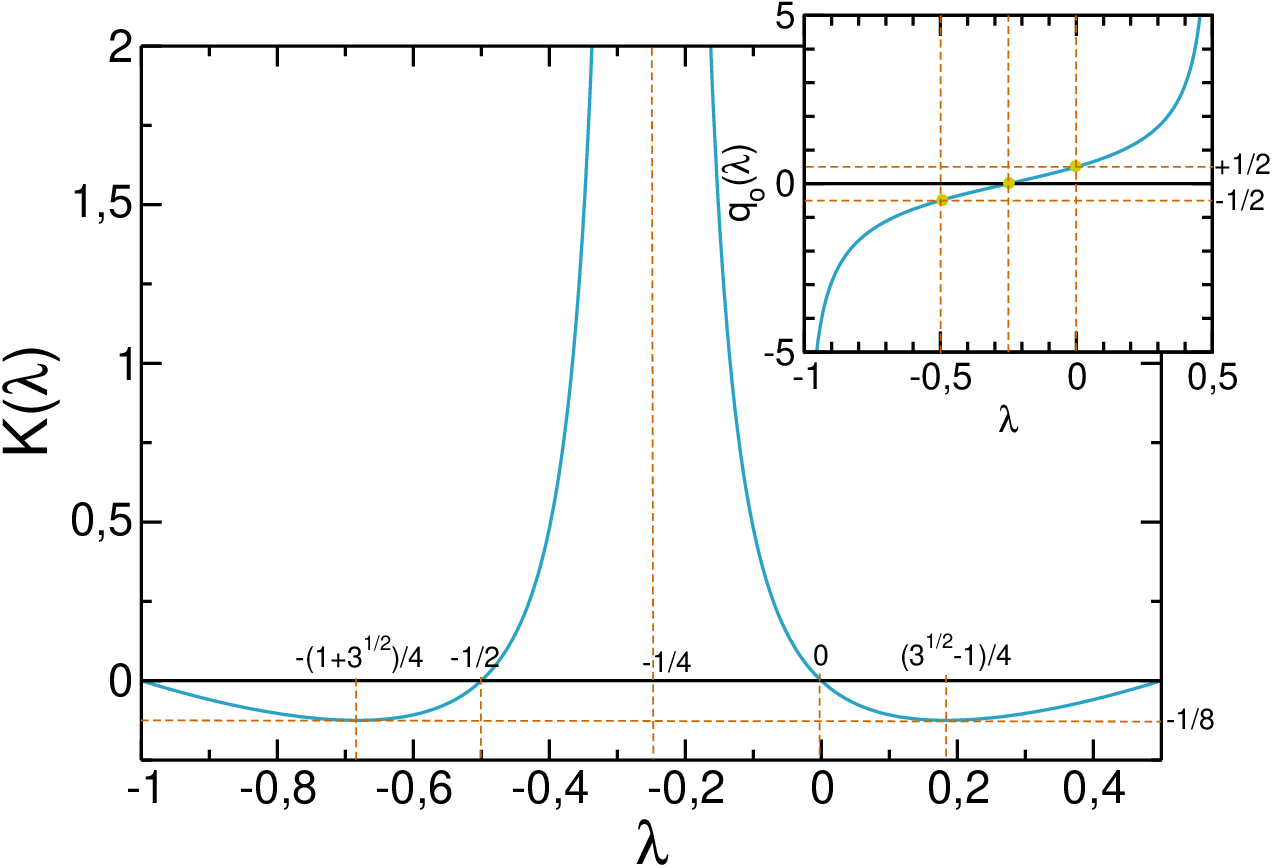
Fig. 1 in the main text shows the predicted for the KMP model. Notice that the large deviation function is zero for , and negative elsewhere. Moreover, for large current fluctuations it decays linearly, for . For a small positive current fluctuation, and
| (60) |
which translates into
| (61) |
for the Legendre transform. Therefore the probability of small current fluctuations is Gaussian in while it becomes exponential for large enough deviations from the average, see eq. (1). It is easy to show that the Gallavotti-Cohen symmetry holds, with
| (62) |
or equivalently
| (63) |
with . Fig. 2 in the main text shows the optimal temperature profiles for different current deviations. Notice that the optimal profile is independent of the sign of the current, i.e. , reflecting the time-reversal symmetry of microscopic dynamics [12, 13]. Finally, Fig. 11 shows, for information purposes, the integration constant as a function of both and , as well as -dependence of .
Appendix B Standard Simulations
In order to see how far standard simulations can go in evaluating current large fluctuations, and to cross-check our results with the more advanced simulation methods described in Appendix C, we performed a large number of steady-state simulations of long duration , with and , measuring the total time-integrated current and accumulating statistics for . Fig. 12 shows the measured obtained for different system sizes and durations . Our simulations for and different times follow closely the Gaussian law obtained from the first two moments prescribed by the additivity principle in this case, namely
This Gaussian behavior is expected for small fluctuations around the average current, see eq. (60), but deviations away from Gaussianity should be already observed in the current range studied, see the theoretical prediction. In particular, the theoretical implies a nonzero third central moment, but we have not found numerical evidence of such a deviation for . This lack of structure stems from the relatively short duration of the simulations for , i.e. our results are not in the diffusive regime ( here) and therefore we have not reached the asymptotic behavior.


We performed two set of simulations in the diffusive regime , namely with and . In the first case there were no events outside the current interval , for which the BD prediction is numerically indistinguishable from the Gaussian one. On the other hand, the case and shows systematic deviations from Gaussian behavior, seemingly compatible with BD theory, see Fig. 12. However, large errorbars resulting from the difficulty of gathering statistics in this rare-fluctuation regime do not allow us to exclude Gaussian behavior. In this way, standard simulation results are inconclusive, as otherwise expected, and the more refined simulation techniques of Appendix C are called for.
We also tested the Gallavotti-Cohen relation in standard simulations for our system. This symmetry implies that
| (64) |
where in this case. Notice that if we assume to be Gaussian with the moments defined above, then one expects . Fig. 13 shows the above quotient as measured for and different values of . It shows a systematic deviation from Gaussian behavior which increases with . However, we do not see clearly , and this means again that our standard simulations are still far from the true asymptotic regime in .
Another prediction of the additivity principle concerns the existence of an optimal temperature profile that the system adopts in order to facilitate a given current fluctuation. We measured in standard simulations the average energy profile during a current large deviation event, obtaining the results shown in Fig. 14. As above, only for small current fluctuations we could gather enough statistics for the data to be significative. In any case, the theoretical optimal profiles compare nicely with data, confirming the existence of a well-defined temperature profile for each current deviation.

We also measured the fluctuations of the total energy in standard simulations. Fig. 15 shows our results in this case. In particular, we measured for and a maximum time and for , in agreement with eq. (26). This figure also shows and build from simulation data for . As in Fig. 9, we see a clear deviation from local equilibrium and a well defined structure not predicted by BD theory. Notice that, again, values of for coincide with the expected average values with no current constraint. The data shown in this figure agree nicely with those measured with the advanced technique in the studied range, see Fig. 9.

Appendix C Evaluation of Large-Deviation Functions
Large deviation functions are very hard to measure in experiments or simulations because they involve by definition exponentially-unlikely events, see eq.(1). Recently, Giardinà, Kurchan and Peliti [20] have introduced an efficient algorithm to measure the probability of a large deviation for observables such as the current or density in stochastic many-particle systems. The algorithm is based on a modification of the underlying stochastic dynamics so that the rare events responsible of the large deviation are no longer rare, and it has been extended for systems with continuous-time stochastic dynamics [21]. Let be the transition rate from configuration to . The probability of measuring a time-integrated current after a time starting from a configuration can be written as
| (65) |
where is the elementary current involved in the transition . For long times we expect the information on the initial state to be lost, . In this limit obeys the usual large deviation principle . In most cases it is convenient to work with the moment-generating function of the above distribution
| (66) | |||||
For long , we have , with . We can now define a modified dynamics, , so
| (67) |
This dynamics is however not normalized, .
We now introduce Dirac’s bra and ket notation, useful in the context of the quantum Hamiltonian formalism for the master equation [23, 24], see also [20, 25]. The idea is to assign to each system configuration a vector in phase space, which together with its transposed vector , form an orthogonal basis of a complex space and its dual [23, 24]. For instance, in the simpler case of systems with a finite number of available configurations (which is not the case for the KMP model), one could write , i.e. all components equal to zero except for the component corresponding to configuration , which is . In this notation, , and a probability distribution can be written as a probability vector
where with the scalar product . If , normalization then implies .

With the above notation, we can write the spectral decomposition , where we assume that a complete biorthogonal basis of right and left eigenvectors for matrix exists, and . Denoting as the largest eigenvalue of , with associated right and left eigenvectors and , respectively, and writing , we find for long times
| (68) |
In this way we have , so the Legendre transform of the current LDF is given by the natural logarithm of the largest eigenvalue of . In order to evaluate this eigenvalue, and given that dynamics is not normalized, we introduce the exit rates , and define the normalized dynamics . Now
| (69) |
This sum over paths can be realized by considering an ensemble of copies (or clones) of the system, evolving sequentially according to the following Monte Carlo scheme [20]:
- I
Each copy evolves independently according to modified normalized dynamics .
- II
Each copy (in configuration at time ) is cloned with rate . This means that, for each copy , we generate a number of identical clones with probability , or otherwise (here represents the integer part of ). Note that if the copy may be killed and leave no offspring. This procedure gives rise to a total of copies after cloning all of the original copies.
- III
Once all copies evolve and clone, the total number of copies is sent back to by an uniform cloning probability .
Fig. 16 sketches this procedure. It then can be shown that, for long times, we recover via
| (70) |
To derive this expression, first consider the cloning dynamics above, but without keeping the total number of clones constant, i.e. forgetting about step III. In this case, for a given history , the number of copies in configuration at time obeys , so that
| (71) |
Summing over all histories of duration , see eq. (69), we find that the average of the total number of clones at long times shows exponential behavior, . Now, going back to step III above, when the fixed number of copies is large enough, we have for the global cloning factors, so and we recover expression (70) for .
In this paper we used the above method to measure the current LDF for the Kipnis-Marchioro-Presutti model in one dimension, described in Section III. For this model the transition rate from a configuration to another configuration , with and the pair defined as in eqs. (18)-(19), can be written as
Here , where is the exponential integral function, or
| (78) |
It appears when integrating over all possible pairs that can result on a given , respectively, see eq. (19) in Section III. It is easy to show that is normalized as it should, so .
In order to measure current fluctuations we need to provide a microscopic definition of the energy current involved in an elementary move. There are many different ways to define this current: the energy exchanged per unit time with one of the boundary heat baths, the current flowing between two given nearest neighbors, or its spatial average, etc. Assuming that energy cannot accumulate in the system ad infinitum[6, 7, 25], all these definitions give equivalent results for the current large deviation function in the long time limit. However, this is not so for some observables different from the large deviation function (e.g. for average profiles measured at the end of the large deviation event; see Ref. [22]). In our case, the following choice turns out to be convenient
That is, we measure the energy current flowing through the bulk of the system. Using this current definition and eq. (C), we may write the modified normalized dynamics , which for reads
| (83) |
with , while for , see eq. (C). The exit rate is given by
| (84) |
In these paper we simulate a system of size , with and , using copies of the system and a maximum time of Monte Carlo steps. For a given initial condition, we average the measured for different times once in the steady state, after a relaxation time of Monte Carlo steps. In addition, we average results over many independent initial conditions, in which local initial energies are randomly drawn according to the Gibbs distribution with temperature parameter corresponding to the linear, steady temperature profile. Fig 17 shows the convergence of in time for a given value of and many different initial conditions. Using the above method, we obtained an accurate measurement of the current large deviation function, see Fig. 3 in Section IV.

Appendix D Time Reversibility and Statistics during a Large Fluctuation
In this Appendix we use the time reversibility of the underlying stochastic dynamics to study the system statistics during a large deviation event and the symmetries of the large deviation function and the associated optimal profiles, using the formalism described in Appendix C. In particular, we describe a relation between system statistics at the end of the large deviation event and for intermediate times. First, consider the probability that the system is in configuration at time with a total time-integrated current . As in the previous appendix, we drop the dependence of this probability on the initial state , which we assume lost for long enough times. This probability obeys the following master equation
| (85) |
which by iterating in time leads to
| (86) |
and it is clear that , see eq. (65) in the previous appendix. Now, is the probability of having a configuration at the end of a large deviation event associated to a current . Defining so that
| (87) |
with , one can easily show that, for long times , , where is the current conjugated to parameter , and is defined in eq. (67). Using the spectral decomposition of Appendix C, it is simple to show that , so the right eigenvector associated to the largest eigenvalue of matrix gives the probability of having any configuration at the end of the large deviation event. Noticing that, for the Monte Carlo algorithm described in the previous appendix, the fraction of clones or copies in state is proportional to for long times, see eq. (71), we deduce that the the average profile among the set of clones yields the mean temperature profile at the end of the large deviation event, .
The initial and final time regimes during a large deviation event show transient behavior which differs from the behavior in the bulk of the large deviation event, i.e. for intermediate times [6]. In particular, as we will show here, midtime and endtime statistics are different, though intimately related as a result of the time reversibility of the microscopic dynamics. Let be the probability that the system was in configuration at time when at time the total integrated current is . Timescales are such that , so all times involved are long enough for the memory of the initial state to be lost. We can write now
| (88) |
where we do not sum over . Defining the moment-generating function of the above distribution, , we can again check that the probability weight of configuration at intermediate time in a large deviation event of current , , is also given by for long times such that , with . In this long-time limit one thus finds
| (89) |
in contrast to , which is proportional to , see above. Here and are the right and left eigenvectors associated to the largest eigenvalue of modified transition rate , respectively. They are different because is not symmetric. In order to compute the left eigenvector, notice that is the right eigenvector of the transpose matrix with eigenvalue . This right eigenvector of can be in turn related to the corresponding right eigenvector of by noticing that the local detailed balance condition holds for the KMP model, guaranteeing the time reversibility of microscopic dynamics. This condition states that , where is an effective equilibrium weight which for the KMP model takes the value with and . Local detailed balance then implies a symmetry between the forward modified dynamics for a current fluctuation and the time-reversed modified dynamics for the negative current fluctuation, i.e. , or in matrix form
| (90) |
where is a diagonal matrix with entries . Eq. (90) implies that all eigenvalues of and are equal, and in particular the largest, so and this proves the Gallavotti-Cohen fluctuation relation. Moreover, if is a right eigenvector of , which can be expanded as , then
| (91) |
is the right eigenvector of associated to the same eigenvalue. In this way, by plugging this into eq. (92) we find
where we assumed real components for the eigenvectors associated to the largest eigenvalue. Equivalently
| (92) |
with a normalization constant. This relation implies that configurations with a significant contribution to the average profile at intermediate times are those with an important probabilistic weight at the end of both the large deviation event and its time-reversed process. Supplementing the above relation with a local equilibrium hypothesis, one can obtain average temperature profiles at intermediate times in terms of profile statistics at the end of the large deviation event.
Acknowledgements.
We thank B. Derrida, J.L. Lebowitz, V. Lecomte and J. Tailleur for illuminating discussions and comments. Financial support from Spanish project FIS2009-08451, AFOSR Grant No. AF-FA-9550-04-4-22910 and University of Granada is also acknowledged.References
- [1] H. Spohn, Large Scale Dynamics of Interacting Particles, Springer-Verlag (1991).
- [2] J. Marro and R. Dickman, Nonequilibrium Phase Transitions in Lattice Models, Cambridge University Press (2005).
- [3] J. -P. Eckmann and D. Ruelle, Rev. Mod. Phys. 57, 617 (1985).
- [4] L. Bertini, A. De Sole, D. Gabrielli, G. Jona-Lasinio and C. Landim, Phys. Rev. Lett. 87, 040601 (2001); Phys. Rev. Lett. 94, 030601 (2005); J. Stat. Mech. P07014 (2007); J. Stat. Phys. 135, 857 (2009).
- [5] T. Bodineau and B. Derrida, Phys. Rev. Lett. 92, 180601 (2004).
- [6] B. Derrida, J. Stat. Mech. P07023 (2007).
- [7] T. Bodineau and B. Derrida, C. R. Physique 8, 540 (2007).
- [8] B. Derrida and A. Gerschenfeld, J. Stat. Phys. 136, 1 (2009); 137, 978 (2009).
- [9] S. Lepri, R. Livi, and A. Politi, Phys. Rep. 377, 1 (2003).
- [10] A. Dhar, Adv. Phys. 57, 457 (2008).
- [11] P.L. Garrido, P.I. Hurtado and B. Nadrowski, Phys. Rev. Lett. 86, 5486 (2001); P.L. Garrido and P.I. Hurtado, Phys. Rev. Lett. 88, 249402 (2002); 89, 079402 (2002); P.I. Hurtado, Phys. Rev. Lett. 96, 010601 (2006); Phys. Rev. E 72, 041101 (2005).
- [12] G. Gallavotti and E.G.D. Cohen, Phys. Rev. Lett. 74, 2694 (1995).
- [13] J.L. Lebowitz and H. Spohn, J. Stat. Phys. 95, 333 (1999).
- [14] Pablo I. Hurtado and Pedro L. Garrido, Phys. Rev. Lett. 102, 250601 (2009).
- [15] R.S. Ellis, Entropy, Large Deviations and Statistical Mechanics, Springer, New York (1985).
- [16] H. Touchette, Phys. Rep. 478, 1 (2009).
- [17] C. Kipnis, C. Marchioro and E. Presutti, J. Stat. Phys. 27, 65 (1982).
- [18] T. Bodineau and B. Derrida, Phys. Rev. E 72, 066110 (2005).
- [19] Pablo I. Hurtado and Pedro L. Garrido, to appear.
- [20] C. Giardinà, J. Kurchan and L. Peliti, Phys. Rev. Lett. 96, 120603 (2006).
- [21] V. Lecomte and J. Tailleur, J. Stat. Mech. P03004 (2007).
- [22] Pablo I. Hurtado and Pedro L. Garrido, J. Stat. Mech. (2009) P02032.
- [23] R.J. Harris and G.M. Schütz, J. Stat. Mech. P07020 (2007).
- [24] G.M. Schütz, in Phase Transitions and Critical Phenomena vol. 19, ed. C. Domb and J.L. Lebowitz, London Academic (2001).
- [25] A. Rákos and R.J. Harris, J. Stat. Mech. P05005 (2008).
- [26] H. Spohn, J. Phys. A 16, 4275 (1983)
- [27] L. Bertini, D. Gabrielli and J.L. Lebowitz, J. Stat. Phys. 121, 843 (2005)