Noise bridges dynamical correlation and topology in coupled oscillator networks

Understanding the relationship between dynamics and network structure is a central issue in interdisciplinary science [1, 2]. Despite the tremendous efforts in revealing the topological effect on a variety of dynamics [3, 4, 5], how to infer the interaction pattern from dynamical behaviors is still challenging as an inverse problem, especially in the absence of the knowledge of nodal dynamics. Some methods aiming to address the inverse problem have been proposed, such as spike classification methods for measuring interactions among neurons from spike trains [6], and approaches based on response dynamics [7], $L1$ norm [8] and noise scaling [9]. For the inverse problem, a basic question is whether sufficient topological information can be obtained from measured time series of dynamics. In this regard, the answer is negative when there is strong synchronization as, in this case, the coupled units behave as a single oscillator and interactions among units vanish so that it is impossible to extract the interaction pattern from measurements.

Quite surprisingly, we find that with the help of noise, in general it becomes possible to precisely identify interactions based solely on the correlations among measured time series of nodes. In this sense, we say that noise bridges dynamics and topology, facilitating inference of network structures. We note that noise is ubiquitous in physical and natural systems and understanding the noise effect on dynamical systems has been a fundamental issue in nonlinear and statistical physics. While there are recent works on the interplay between collective dynamics and topology of complex systems under noise [10, 11, 12] and on predicting node degrees for complex networks [9], taking advantage of noise to predict the full connecting topology of an unknown complex network is an outstanding question. Addressing this question not only is fundamental to nonlinear science, but also can have significant applications in diverse areas such as computer networks, biomedical systems, neuroscience, socio-economics, and defense.

In this Letter, we present a general and powerful method to precisely identify links among nodes based on the noise-induced relationship between dynamical correlation and topology. Analytically, we find that there exists a one-to-one correspondence between the dynamical correlation matrix of nodal time series and the connection matrix of structures, due to the presence of noise. This finding enables an accurate prediction of network topology from time series. Numerical simulations are performed using four typical dynamical systems, together with several model and real networks. For all cases examined, comparisons between the original and the predicted topology yield uniformly high success rate of prediction. The advantages of our noise-based method are then: (i) high accuracy and efficiency, (ii) generality with respect to node dynamics and network structures, (iii) no need for control, and (iv) applicability even when there is weak coherence in the collective dynamics.

Our general approach to bridging dynamical correlation and topology is, as follows. We consider $N$ nonidentical oscillators, each of which satisfies $\dot{\mathbf{x}}_{i}=\mathbf{F}_{i}(\mathbf{x}_{i})$ in the absence of coupling, where $\mathbf{x}_{i}$ denotes the $d$-dimensional state variable of the $i$th oscillator. Under noise, the dynamics of the whole coupled-oscillator system can be expressed as:

where $c$ is the coupling strength, $\mathbf{H}:\mathbb{R}^{d}\rightarrow\mathbb{R}^{d}$ denotes the coupling function of oscillators, $\eta_{i}$ is the noise term, $L_{ij}=-1$ if $j$ connects to $i$ (otherwise $0$) for $i\neq j$ and $L_{ii}=-\sum_{j=1,j\neq i}^{N}L_{ij}$. Due to nonidentical oscillators and noise, an invariant synchronization manifold does not exist. Let $\mathbf{\bar{x}}_{i}$ be the counterpart of $\mathbf{x}_{i}$ in the absence of noise, and assume a small perturbation $\xi_{i}$, we can write $\mathbf{x}_{i}=\mathbf{\bar{x}}_{i}+\xi_{i}$. Substituting this into Eq. (1), we obtain:

where $\xi=[\xi_{1},\xi_{2},\ldots,\xi_{N}]^{T}$ denotes the deviation vector, $\eta=[\eta_{1},\eta_{2},\ldots,\eta_{N}]^{T}$ is the noise vector, $\mathbf{\hat{L}}$ names the Laplacian matrix of coupling $\{L_{ij}\}$, $D\mathbf{\hat{F}}(\mathbf{\bar{x}})=\mathrm{diag}[D\mathbf{\hat{F}}_{1}(\mathbf{\bar{x}}_{1}),D\mathbf{\hat{F}}_{2}(\mathbf{\bar{x}}_{2}),\cdots,D\mathbf{\hat{F}}_{N}(\mathbf{\bar{x}}_{N})]$ ($D\mathbf{\hat{F}}_{i}$ are $d\times d$ Jacobian matrices of $\mathbf{F}_{i}$), $\otimes$ denotes direct product, and $D\mathbf{\hat{H}}$ is the Jacobian matrix of the coupling function $\mathbf{H}$.

Denoting the dynamical correlation of oscillators $\langle\xi\xi^{T}\rangle$ as $\mathbf{\hat{C}}$, wherein $C_{ij}=\langle\xi_{i}\xi_{j}\rangle$ and $\langle\cdot\rangle$ is time average, we have

where $\mathbf{\hat{A}}=-D\mathbf{\hat{F}}(\mathbf{\bar{x}})+c\mathbf{\hat{L}}\otimes D\mathbf{\hat{H}}(\mathbf{\bar{x}})$. To obtain the expression of $\langle\eta\xi^{T}\rangle$ and $\langle\xi\eta^{T}\rangle$, we get the solution $\xi(t)$ from Eq. (2): $\xi(t)=\mathbf{\hat{G}}(t-t_{0})\xi(t_{0})+\int_{t_{0}}^{t}dt^{\prime}\mathbf{\hat{G}}(t-t^{\prime})\eta(t^{\prime}),$ where $\mathbf{\hat{G}}(t)=\exp(-\mathbf{\hat{A}}t)$. In the absence of divergence of state variables, $\mathbf{\hat{G}}(\infty)=0$. Setting $t_{0}\rightarrow-\infty$, without loss of generality, we have $\xi(t)=\int_{-\infty}^{t}\mathbf{\hat{G}}(t-t^{\prime})\eta(t^{\prime})dt^{\prime}$. Note that $\mathbf{\hat{G}}(0)=\mathbf{\hat{I}}$, we hence obtain $\langle\xi\eta^{T}\rangle=\int_{-\infty}^{t}\mathbf{\hat{G}}(t-t^{\prime})\langle\eta(t)\eta^{T}(t^{\prime})\rangle dt^{\prime}=\int_{-\infty}^{t}\mathbf{\hat{G}}(t-t^{\prime})\mathbf{\hat{D}}\delta(t-t^{\prime})dt^{\prime}=\mathbf{\hat{D}}/2,$ where $\mathbf{\hat{D}}$ is the covariance matrix of noise. Analogously, we can obtain $\langle\eta\xi^{T}\rangle=\mathbf{\hat{D}}/2$. Therefore, Eq. (3) can be simplified to:

Since $\mathbf{\hat{A}}=-D\mathbf{\hat{F}}(\mathbf{\bar{x}})+c\mathbf{\hat{L}}\otimes D\mathbf{\hat{H}}(\mathbf{\bar{x}})$, the above equality reveals a general relationship between the dynamical correlation $\mathbf{\hat{C}}$ and the connecting matrix $\mathbf{\hat{L}}$ in the presence of noise as characterized by $\mathbf{\hat{D}}$. The general solution of $\mathbf{\hat{C}}$ can be written as $\mbox{vec}(\mathbf{\hat{C}})=\mbox{vec}(\mathbf{\hat{D}})/(\mathbf{\hat{I}}\otimes\mathbf{\hat{A}}+\mathbf{\hat{A}}\otimes\mathbf{\hat{I}})$, where $\mbox{vec}(\mathbf{\hat{X}})$ is a vector containing all columns of matrix $\mathbf{\hat{X}}$ [13].

For illustrative purpose, we consider one-dimensional state variable and linear coupling such that $D\mathbf{\hat{H}}=1$, with Gaussian white noise $\mathbf{\hat{D}}=\sigma^{2}\mathbf{\hat{I}}$, and further regard the intrinsic dynamics $D\mathbf{\hat{F}}$ as small perturbations. Then Eq. (4) can be simplified to $\mathbf{\hat{L}\hat{C}}+\mathbf{\hat{C}}\mathbf{\hat{L}}^{T}=\sigma^{2}\mathbf{\hat{I}}/c$. For an undirected network with symmetric coupling matrix, the solution of $\mathbf{\hat{C}}$ can be expressed as:

where $\mathbf{\hat{L}}^{\dagger}$ denotes the pseudo inverse of the Laplacian matrix. We note that the dynamic correlation matrix $\mathbf{\hat{C}}$ is closely related to the network connection matrix $\mathbf{\hat{L}}$, which can be used to infer network structures when no knowledge about the nodal dynamics is available. In fact, $\mathbf{\hat{C}}$ acts as the “Green’s function” of the network and can be expressed as some kind of path integral associated with the underlying network topology (see [14]), as follows:

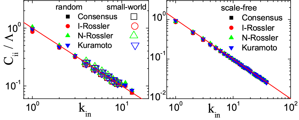
where $\mathbf{path}$ means all paths from $j$ to $i$, and $m$ denotes the nodes on them. This path-integral representation is extremely useful for revealing the direct relation between autocorrelation $C_{ii}$ in the matrix $\mathbf{\hat{C}}$ and the local structure $k_{i}$. In particular, for $n$th-order approximation, we count all paths whose lengths are equal to or less than $n$. Under second-order approximation, we have

where mean-field approximation is applied and $\Gamma_{i}$ denote the neighbors of node $i$. This dependence of the autocorrelation $C_{ii}$ on the degree $k_{i}$, under the second-order approximation is consistent with the recently discovered noise-induced algebraic scaling law in Ref. [9], derived there by a power-spectral analysis.

To provide numerical support for the validity and generality of our theoretical results on the relationship between dynamical correlation and topology, we consider a number of model and real-world network structures by using four typical dynamical systems, as follows. (i) Consensus dynamics [15]: $\dot{x}_{i}=c\sum_{j=1}^{N}P_{ij}(x_{j}-x_{i})+\eta_{i}$; (ii) Identical Rössler dynamics [16] (I-Rössler): $\dot{x}_{i}=-y_{i}-z_{i}+c\sum_{j=1}^{N}P_{ij}(x_{j}-x_{i})+\eta_{i}$, $\dot{y}_{i}=x_{i}+0.2y_{i}+c\sum_{j=1}^{N}P_{ij}(y_{j}-y_{i})$, $\dot{z}_{i}=0.2+z_{i}(x_{i}-9.0)+c\sum_{j=1}^{N}P_{ij}(z_{j}-z_{i})$; (iii) Nonidentical Rössler dynamics [17] (N-Rössler): $\dot{x}_{i}=-\omega_{i}y_{i}-z_{i}+c\sum_{j=1}^{N}P_{ij}(x_{j}-x_{i})+\eta_{i}$, $\dot{y}_{i}=\omega_{i}x_{i}+0.2y_{i}+c\sum_{j=1}^{N}P_{ij}(y_{j}-y_{i})$, $\dot{z}_{i}=0.2+z_{i}(x_{i}-9.0)+c\sum_{j=1}^{N}P_{ij}(z_{j}-z_{i})$, where $\omega_{i}$ governs the natural frequency of an individual oscillator $i$ and is randomly chosen from a range $[a_{1},a_{2}]$; (iv) Kuramoto phase oscillators [18]: $\dot{\theta_{i}}=\omega_{i}+c\sum_{j=1}^{N}P_{ij}\sin(\theta_{j}-\theta_{i})+\eta_{i}$, where $\theta_{i}$ and $\omega_{i}$ are the phase and natural frequency of node $i$.

Numerical simulations are carried out to predict the entire network structure based solely on time series, utilizing the one-to-one correspondence between the dynamical correlation and Laplacian matrix of topology. From Eq. (5), we have $\mathbf{\hat{L}}=[\sigma^{2}/(2c)]\mathbf{\hat{C}}^{\dagger}$, where $\mathbf{\hat{L}}$ contains full information about the network topology, and $\mathbf{\hat{C}}^{\dagger}$ is the pseudo inverse. The matrix $\mathbf{\hat{C}}$ can be obtained from time series as $C_{ij}=\langle[\mathrm{x}_{i}(t)-\mathrm{\bar{x}}(t)]\cdot[\mathrm{x}_{j}(t)-\mathrm{\bar{x}}(t)]\rangle$, where $\mathrm{\bar{x}}(t)=(1/N)\sum_{i=1}^{N}\mathrm{x}_{i}(t)$. For Kuramoto oscillators, $\mathrm{x}_{i}(t)$ denotes the phase variable $\theta(t)$ and for the Rössler dynamics, $\mathrm{x}_{i}(t)$ is the $x$ component of the $i$th oscillator [19]. After $\mathbf{\hat{C}}$ is constructed, we are able to obtain $\mathbf{\hat{L}}$ through the pseudo inverse.

Figure 1 shows the distribution of elements of $[\sigma^{2}/(2c)]\mathbf{\hat{C}}^{{\dagger}}$. We observe a bimodal distribution with one peak centered at $-1$ corresponding to existent links and the other peak centered at zero corresponding to zero elements in $\mathbf{\hat{L}}$. There are also some positive values in the distribution that disperse on the right side of the peak about zero, which are due to the diagonal components in $\mathbf{\hat{L}}$. We focus on non-diagonal elements in $\mathbf{\hat{L}}$. If $\mathbf{\hat{L}}$ were reconstructed perfectly from $[\sigma^{2}/(2c)]\mathbf{\hat{C}}^{{\dagger}}$, the two peaks would be very sharp. A threshold can be set to distinguish existent from non-existent links by using Eq. (7). In particular, from Eq. (7), we have $S\equiv\sum_{i=1}^{N}1/C_{ii}=2cl^{2}/[\sigma^{2}(N+l)]$, where $l=\sum_{i=1}^{N}k_{i}=N\langle k\rangle$ is twice the total number of links. We can calculate $l$ through $l=(S\sigma^{2}+\sqrt{S^{2}\sigma^{4}+8cNS\sigma^{2}})/4c$ and keep its integral part. We then rank all elements of the matrix $\mathbf{\hat{C}}^{{\dagger}}$ (or matrix $[\sigma^{2}/(2c)]\mathbf{\hat{C}}^{{\dagger}}$) in an ascending order. For convenience, we denote the ascending-ordered matrix elements by $C_{m}^{{\dagger}}$, for $m=1,\ldots,N^{2}$. The threshold $C_{M}^{{\dagger}}$ (or $[\sigma^{2}/(2c)]C_{M}^{{\dagger}}$) is chosen such that $\sum^{M}_{m=1}\Phi(C_{m}^{{\dagger}})=l$, where $\Phi(C_{m}^{{\dagger}})$ is the unnormalized distribution of $C_{m}^{{\dagger}}$. This means the rank of $C_{M}^{{\dagger}}$ is $l$ in the queue of ascending-ordered matrix elements $C_{m}^{{\dagger}}$. Then the connection matrix can be obtained by setting all elements in $\mathbf{\hat{C}}^{\dagger}$ with values above the threshold $C_{M}^{{\dagger}}$ to be zero and others to be $-1$, the latter corresponding to existent links. As shown in Fig. 1, for different model and real-world networks, thresholds so determined are able to successfully separate the two peaks in the distributions of elements of $\mathbf{\hat{C}}^{{\dagger}}$, which in turn leads to predictions of links with high success rates for various node dynamics, as displayed in Table 1. Alternatively, the threshold can be empirically determined by the largest gap between the two peaks, and we have obtained essentially the same success rates. Table 2 exemplifies the success rates of our method for different values of the average degree $\langle k\rangle$ for different types of networks. We see that the success rate increases with $\langle k\rangle$.

For directed networks, there is no unique solution for $\mathbf{\hat{L}}$ from $\mathbf{\hat{C}}$, because the asymmetric $\mathbf{\hat{L}}$ has a twofold degree of freedom as that of symmetric $\mathbf{\hat{C}}$. Thus, the global structure of directed networks cannot be inferred solely depending on the correlation. However, Eq. (7) is satisfied by replacing node degree with in-degree, so that we still can infer the local structure, the in-degree of each node, through $k_{in}^{i}\sim C_{ii}^{-1}$. As shown in Fig. 2, theory agrees well with numerical results.

In conclusion, we have discovered a general relation between the dynamical correlation among oscillators and the underlying topology in the presence of noise. The correlation matrix is inversely proportional to the Laplacian matrix that contains full information about the network structure. Reconstruction of the full network topology based on time series then becomes possible, particularly for undirected networks. We have provided strong numerical support by using four types of nodal dynamics together with several model and real-world network structures. We find that the full network topology can be predicted with high success rate and efficiency for all considered cases. Besides high success rates, advantages making our method attractive and powerful include generality for a variety of nodal dynamics and network structures, validity in the existence of weak coherence, applicability in the absence of knowledge about nodal dynamics, and no need to control nodal dynamics as in some existing method. We hope that our method can be widely applied for inferring network structures and inspire further research towards the understanding of noise effects on networked dynamical systems.

We thank anonymous referees for valuable suggestions on theoretically determining thresholds. WXW and YCL are supported by AFOSR under Grant No. FA9550-07-1-0045.

References

- [1] M. E. J. Newman, SIAM Rev. 45, 167 (2003).
- [2] S. Boccaletti, V. Latora, Y. Moreno, M. Chavez, and D. U. Hwang, Physics Reports 424, 175 (2006).
- [3] For spreading, see, for example, M. Boguñá and R. Pastor-Satorras, Phys. Rev. E 66, 047104 (2002); M. Boguñá, R. Pastor-Satorras, and A. Vespignani, Phys. Rev. Lett. 90, 028701 (2003).
- [4] For synchronization, L. M. Pecora and T. L. Carroll, Phys. Rev. Lett. 80, 2109 (1998); X. F. Wang and G. Chen, Int. J. Bif. Chaos Appl. Sci. Eng. 12, 187 (2002); T. Nishikawa, A. E. Motter, Y.-C. Lai, and F. C. Hoppensteadt, Phys. Rev. Lett. 91, 014101 (2003).
- [5] For vibration, J. Ren and B. Li, Phys. Rev. E 79, 051922 (2009).
- [6] R. Gütig, A. Aertsen, and S. Rotter, Neural Comput. 14, 121 (2002); G. Pipa and S. Grün, Neurocomputing 52, 31 (2003).
- [7] M. Timme, Phys. Rev. Lett. 98, 224101 (2007);
- [8] D. Napoletani and T. D. Sauer, Phys. Rev. E 77, 026103 (2008).
- [9] W.-X. Wang, Q. Chen, L. Huang, Y.-C. Lai, and M. A. F. Harrison, Phys. Rev. E 80, 016116 (2009).
- [10] N. J. McCullen, T. Mullin, and M. Golubitsky, Phys. Rev. Lett. 98, 254101 (2007)
- [11] J.-N. Teramae and T. Fukai, Phys. Rev. Lett. 101, 248105 (2008)
- [12] S. Meloni, J. Gómez-Gardeñes, V. Latora, and Y. Moreno, Phys. Rev. Lett. 100, 208701 (2008).
- [13] R. A. Horn and C. R. Johnson, Topics in Matris Analysis (Cambridge Uni. Press, Cambridge, U.K., 1999).
- [14] We can decompose into two parts: , where is the adjacency matrix with if node connects to (otherwise ), and , where is the degree of node . The matrix can thus be expressed in a series: . For the second term , if nodes connects to , its element is and otherwise 0. For the third term , if there are multiple two-step paths connecting to through node or , , , its element values .
- [15] R. Olfati-Saber, Proc. of the IEEE, 95, 215 (2007).
- [16] O. E. Rössler, Phys. Lett. A 57, 397 (1976).
- [17] G. V. Osipov, A. S. Pikovsky, M. G. Rosenblum, and J. Kurths, Phys. Rev. E 55, 2353 (1997).
- [18] Y. Kuramoto, Chemical Oscillations, Waves and Turbulence (Springer-Verlag, Berlin, 1984); S. H. Strogatz, Physica D 143, 1 (2000).
- [19] can also be the or component with noise in Rössler dynamics. We have examined the success rate by using the time series of or for various networks. High success rates are obtained as well, similar to the results by using the -component.
- [20] SREL (SRNL) is defined as the ratio of the number of successfully predicted existent (non-existent) links to the total number of existent (non-existent) links.
- [21] P. Erdős and A. Rényi, Publ. Math. (Debrecen) 6, 290 (1959).
- [22] D. J. Watts and S. H. Strogatz, Nature (London) 393, 440 (1998).
- [23] A.-L. Barabási and R. Albert, Science 286, 509 (1999).
- [24] http://www.orgnet.com/cases.html.
- [25] W. W. Zachary, J. Anthropol. Res. 33, 452 (1977).
- [26] M. Girvan and M. E. J. Newman, Proc. Natl. Acad. Sci. USA 99, 7821 (2002).
- [27] R. Milo, S. Itzkovitz, N. Kashtan, R. Levitt, S. Shen-Orr, I. Ayzenshtat, M. Sheffer, and U. Alon, Science 303, 1538 (2004).
- [28] D. Lusseau, K. Schneider, O. J. Boisseau, P. Haase, E. Slooten, and S. M. Dawson, Behav. Ecol. Sociobiol. 54, 396 (2003).