A semi-Dirac point in the Hofstadter spectrum

In zero field, due to the staggered potential, the Hamiltonian has a $2\times 2$ structure

where we introduce the dimensionless parameter $r=\Delta_{s}/(2t)=\Delta_{s}/2$, and where we choose from now $t=a=\hbar=e=1$. Therefore the zero field spectrum is given by

As shown in Fig.3, the spectrum consists of two bands which overlap in energy. The lower band extends from $\epsilon_{l}^{min}=-2-2\sqrt{1+r^{2}}$ to $\epsilon_{l}^{max}=2-2r$, with two saddle points (which yields logarithmic singularities in the density of states) at energies $\epsilon_{l}^{s1}=-2-2r$ and $\epsilon_{l}^{s2}=+2-2\sqrt{1+r^{2}}$. Symmetrically, the upper band extends from $\epsilon_{u}^{min}=-2+2r$ to $\epsilon_{u}^{max}=2+2\sqrt{1+r^{2}}$, with two saddle points (with logarithmic singularities) at energies $\epsilon_{u}^{s1}=-2+2\sqrt{1+r^{2}}$ and $\epsilon_{u}^{s2}=2+2r$. The position of these points is shown on Fig.(4) on a plot of the density of states.

In each band, the saddle points separate regions with open orbits (for energies between the two saddle points) and closed orbits. When $\Delta_{s}=0$, all orbits are closed and the total bandwidth for incommensurate fluxes is zero. This can be qualitatively understood on semiclassical grounds: all closed orbits are quantized and magnetic breakdown induces tunneling between orbits which are all quantized.[25] When $\Delta_{s}$ increases, there are open orbits which are not quantized and the total bandwidth for incommensurate fluxes increases like the number of open orbits.[25] This qualitatively explains why the spectrum is more and more dense when $\Delta_{s}$ increases.

At low magnetic field ($\varphi\ll 1$), the energy levels near the extrema of the band, are grouped into linear Landau levels (Fig.2). Their spectrum is obtained from a low energy expansion of the dispersion relation (9) near ${\boldsymbol{k}}=0$:

leading to a cyclotron mass $m_{0}=(1+r^{2})^{1/4}/2$ and therefore to a set of Landau levels given by ($B=2\pi\varphi$ in our notations)

which describes properly the evolution of the Landau levels at the extrema of the spectrum (Figs.2).

Figure(2.b) shows that, in the middle of the band and for a finite $\Delta_{s}$, two set of Landau levels intermix. This is emphasized in the enlargement displayed in Fig.(5). This structure is easily understood by looking at the zero field spectrum, displayed on Fig.(3). When $0<r<1$, the spectrum is formed of two overlapping bands. The maximum of the lower band is located at energy $\epsilon=2(1-r)$ and the minimum of the upper band has energy $\epsilon=-2(1-r)$. An expansion around these energies gives

where ${\boldsymbol{q}}_{\pm}$ are deviations respectively to the points $(\pi/2,0)$ and $(\pi/2,\pi)$. Therefore the cyclotron mass scales as $m_{0}=\sqrt{r}/2$, and the two sets of Landau levels are given by

When $r=1$, the two sets of Landau levels separate (2.c).

For $\varphi=p/q=1/2$, the Hamiltonian has the form

with $r=\Delta_{s}/2$. The energy spectrum given by

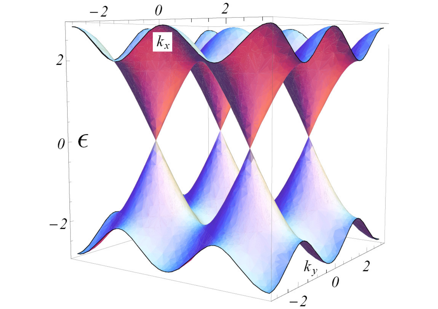
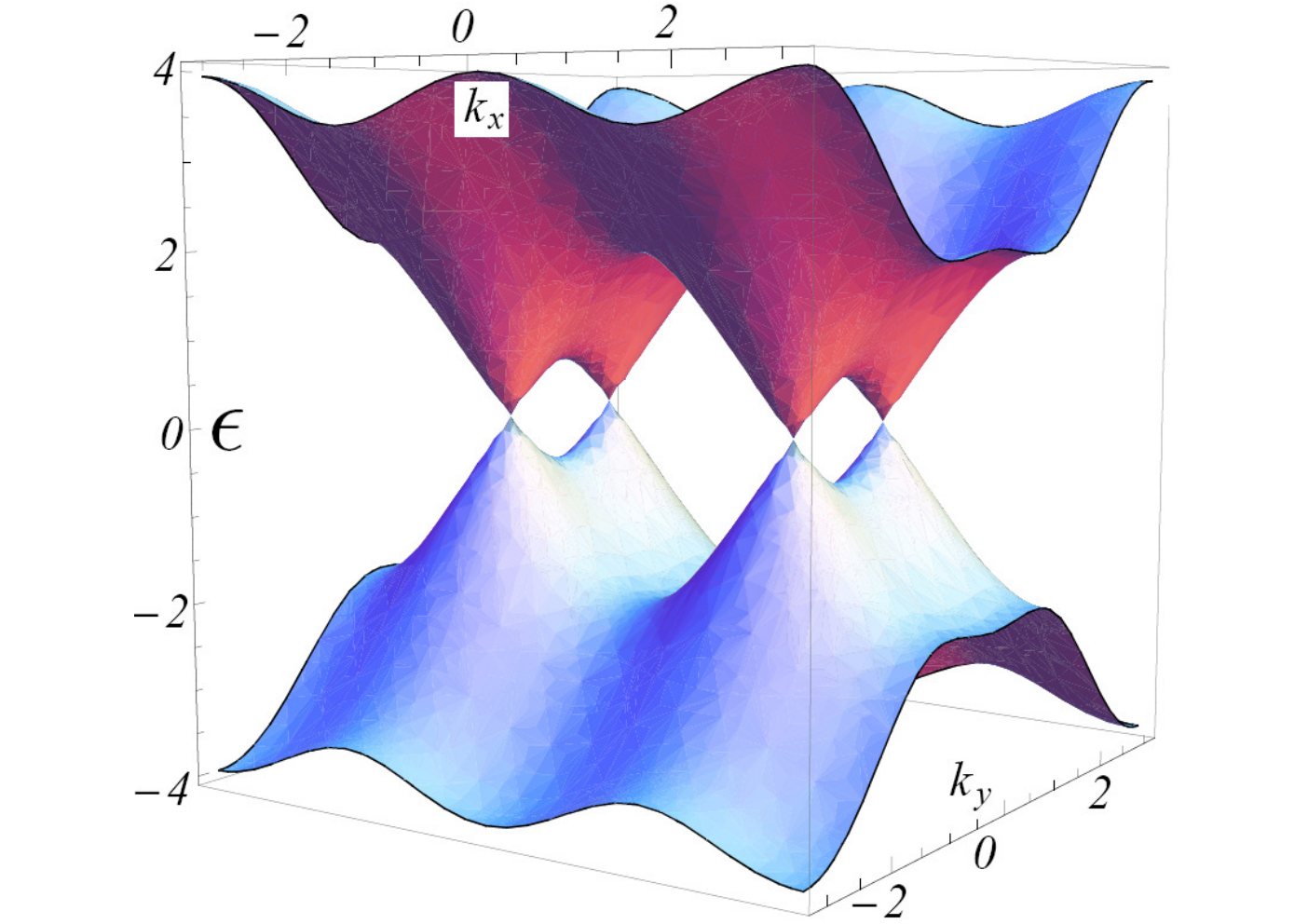
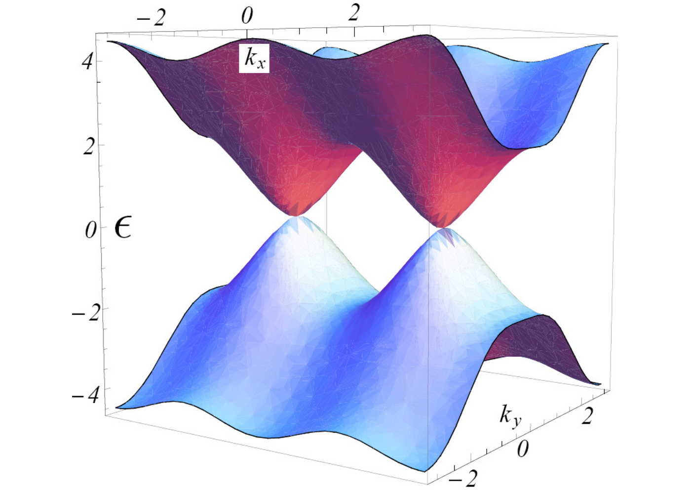
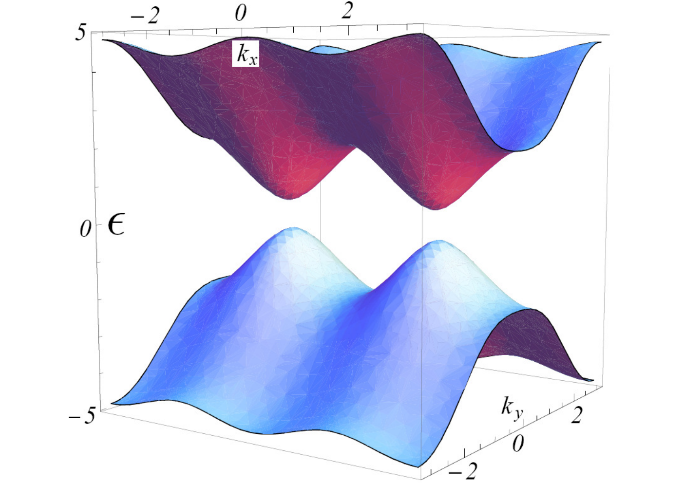
is plotted on Fig.(6) for different values of $r$. It exhibits a pair of Dirac points and their merging occurs when $r=1$.

An expansion of the dispersion relation (15) near its extrema at ${\boldsymbol{k}}_{m}=(0,\pi)$ gives (${\boldsymbol{q}}={\boldsymbol{k}}-{\boldsymbol{k}}_{m}$)

The cyclotron mass $m_{0}$ is therefore

so that in low ”flux” $f$ :

This study is the central point of our paper. When $r=0$, the energy vanishes at the two inequivalent points ${\boldsymbol{D}}_{\xi}=(\pi/2,\xi\pi/2)$ where $\xi=\pm 1$ is the valley index. In the vicinity of these two points, writing ${\boldsymbol{k}}={\boldsymbol{D}}_{\xi}+{\boldsymbol{q}}$, the Hamiltonian can be expanded as

In each valley, the dispersion relation around ${\boldsymbol{D}}_{\xi}$ is

as can be seen on Fig.(6.a).

We now apply a finite uniaxial staggered potential $\Delta_{s}\neq 0$. The Dirac points move and are now located at the positions ${\boldsymbol{D}}_{\xi}=(\pi/2,\xi\arccos r)$ (see Fig.6.b) . A second order expansion around these two points leads to

with a dispersion relation at small ${\boldsymbol{q}}$ of the form

with $c_{x}=2$ and $c_{y}=2\sqrt{1-r^{2}}$.

When $r$ is increased, the two cones become anisotropic because the velocity along the $y$ direction relating the two cones is reduced (Fig.6.b). When $r=1$, the two cones have merged into a single one at the point ${\boldsymbol{D}}_{0}=(\pi/2,0)$ (Fig.6.c), and the Hamiltonian becomes

leading to the ”hybrid” dispersion relation

Quite remarkably, this dispersion relation is linear in one direction, and quadratic in the other. The study of this semi-Dirac point has been the subject of a series of recent works [3, 4, 5, 6, 7, 8, 9, 10, 26] and the present problem constitutes a new realization of this merging.

We now wish to describe the physics of the merging, using the effective Hamiltonian

with $q_{\parallel}=q_{y}$ and $q_{\perp}=q_{x}$. Within the rotation ${\cal H}_{u}={\cal R}\ {\cal H}\ {{\cal R}^{-1}}$ where ${\cal R}=1/\sqrt{2}(\mathbbm{1}-i\sigma_{y})$, the Hamiltonian $\cal H$ is identical to the one ${\cal H}_{u}$ (see Eq.1) that has been recently introduced to describe the merging of Dirac points in a $2D$ crystal with time-reversal and inversion symmetries. When $m^{*}\Delta>0$, there is a gap in the spectrum. Comparison between (25) and the expansion of (14) near ${\boldsymbol{D}}_{0}$ implies that $\Delta=2(r-1)$. When $m^{*}\Delta<0$, the spectrum has two Dirac points separated by $2\sqrt{-2m^{*}\Delta}$ and the velocity $c_{\parallel}$ near these Dirac points is $c_{\parallel}=\sqrt{-2\Delta/m^{*}}$.

In order to quantitatively describe the merging of the Dirac points from the Hofstadter spectrum ($r=0$) to the topological transition $(r=1)$, we choose to fix the velocities $c_{\parallel}=c_{y}=2\sqrt{1-r^{2}}$ and $c_{\perp}=c_{x}=2$. Then, the mass $m^{*}$ has to be fixed as $m^{*}=-2\Delta/c_{\parallel}^{2}=1/(1+r)$. The position of the Dirac points is given by $q_{D}=\pm 2\sqrt{{1-r\over 1+r}}$ slightly different from the real position $q_{D}=\pm\arccos r$ (see ref. 9, for a discussion on this choice).

Using the universal Hamiltonian (25) whose properties are known in a magnetic field, we now describe the evolution of the spectrum when approaching the merging.

When $r$ is small, the spectrum near $\epsilon=0$ can still be described as two independent cones with modified velocities $c_{\perp}=2$ and $c_{\parallel}=2\sqrt{1-r^{2}}$. It is known that in this case,[27] the spectrum is quantized in two-fold degenerate (due to the valley degeneracy) Landau levels with the dispersion relation $\epsilon_{n}=\pm\sqrt{2nc_{\parallel}c_{\perp}eB}$. In our notations, this gives

as confirmed on Figs.(7.a,b). When $r$ increases, the domain of validity of this expression is reduced. As seen in Figs.(2.b) and (7.b), the two-fold degeneracy of the Landau levels is removed when $f$ is increased (in particular the $n=0$ level), until, for $r=1$, the degeneracy is completely removed, with a new field dependence of the levels.

When $r=0$, the Landau levels are doubly degenerate, due to the valley degeneracy of the two Dirac points. When $r$ increases, the two valleys become coupled and the degeneracy is progressively lifted. The spectrum in the vicinity of $\varphi=1/2$, can be described using semiclassical arguments. It can be obtained from Bohr-Sommerfeld quantization ${\cal S}=2\pi(n+\gamma)eB$, where ${\cal S}$ is the area of a cyclotron orbit of energy $\epsilon$ in reciprocal space.

We have to distinguish two regimes (figure 6.b). In the low energy regime $\epsilon<-\Delta=2(1-r)$, this is the area enclosed by one of the two degenerate iso-energy lines encircling one Dirac point. For the Hamiltonian (1), this area has been calculated in ref. 9. Moreover, it has been argued that due to a Berry phase $\pm\pi$ around each Dirac point, the mismatch factor $\gamma$ is $0$. Therefore we find

where $K(x)$ and $E(x)$ are complete elliptic integrals of the first and second kinds, respectively,[28] and $R(x)=\sqrt{2x/(x-1)}$. In the limit $\epsilon\ll-\Delta$, one recovers (26).

In the high energy regime $\epsilon>-\Delta$, that is above the saddle point, the area enclosed by an iso-energy line encircles the two Dirac points so that, due to the cancellation of Berry phases, the mismatch factor $\gamma$ is now $1/2$. The calculation of the area ${\cal S(\epsilon)}$ is this regime gives the semiclassical quantization rule

In the limit $\Delta\rightarrow 0$, one recovers (31). It is shown on Figs.(7), that this semiclassical approximation fits very well the numerical calculations, except in the vicinity of the line $\epsilon=-\Delta$ corresponding to the saddle point separating the two Dirac points (Fig.6).

To go beyond this semiclassical picture, we may explicitly diagonalize the Hamiltonian (25) in a magnetic field. Using the Landau gauge $A_{\parallel}=Bx$, and performing the Peierls substitution $q_{\parallel}-eBx$, one finds that the eigenvalues $\epsilon_{n}$ are solutions of an effective Schrödinger equation (see details in refs. [7, 9])

where $P=\left({2c_{\perp}\over m^{*}\omega_{c}^{2}}\right)^{1/3}q_{\perp}$ and $X=\left({m^{*}\omega_{c}^{2}\over 2c_{\perp}}\right)^{1/3}x$ are respectively dimensionless momentum and position ($[X,P]=i$). We have introduced the dimensionless parameter $\delta=\Delta/\left({m^{*}\omega_{c}^{2}c_{\perp}^{2}\over 2}\right)^{1/3}$. In our case, this is a unique fonction of the flux $f$ and of the parameter $r$ describing the merging :

Eq. (29) is an effective Schrödinger equation for a particle in a double well potential $V(X)=(\delta+X^{2})^{2}-2X$. It has been extensively studied in ref. 9, where its eigenvalues are plotted as a function of the unique parameter $\delta$. Let us recall here its main characteristics. When $\delta<<0$, the two wells of the potential are well separated, one recovers a $\sqrt{nf}$ spectrum of degenerate levels, properly described by eq. (26), with an excellent fit of the butterfly spectrum near $\varphi=1/2$, $\epsilon=0$ (Fig.7.a). When $-\delta$ is decreased, that is when $r$ or $f$ is increasd, the potential barrier between the two wells is reduced, and the tunneling between valleys becomes important. Therefore the two-fold degeneracy of the levels is removed, as seen on Figs.(7.b,c).

When $\delta=0$, that is $r=1$, the spectrum exhibits a single ”semi-Dirac” point. The effective potential $V(X)$ is now a quartic potential $V(X)=X^{4}-2X$. In ref. 3, a simple WKB quantization argument leads to $\epsilon=\pm A(mc_{\perp})^{1/3}[(n+1/2)\omega_{c}]^{2/3}$, where $\omega_{c}=eB/m^{*}$ and $A=3^{2/3}\pi/\Gamma(1/4)^{4/3}$. Using the values of the parameters mentioned above, we expect, at the critical point

with $G=2[36\pi^{5}/\Gamma(1/4)^{4}]^{1/3}\simeq 7.99$. This approximation is quite good as soon as $n>1$. However, it has been shown in ref. 3, that for the ground state, the prefactor has to be multiplied by a factor $g_{0}\simeq 0.808$.[3] Fig.(7.a) shows a remarkable agreement with the semiclassical calculation.

References

- [1] P.R. Wallace, Phys. Rev. 71, 622 (1947)
- [2] For a review see A. H. Castro Neto, F. Guinea, N. M. R. Peres, K. S. Novoselov and A. K. Geim, Rev. Mod. Phys. 81, 109 (2009)
- [3] P. Dietl, F. Piéchon and G. Montambaux, Phys. Rev. Lett. 100, 236405 (2008)
- [4] Y. Hasegawa, R. Konno, H. Nakano and M. Kohmoto, Phys. Rev. B 74, 033413 (2006)
- [5] V. M. Pereira, A. H. Castro Neto and N. M. R. Peres, Phys. Rev. B 80, 045401 (2009)
- [6] B. Wunsch, F. Guinea and F. Sols, New J. Phys. 10, 103027 (2008)
- [7] G. Montambaux, F. Piéchon, J.-N. Fuchs and M.O. Goerbig, Phys. Rev. B 80, 153412 (2009)
- [8] K. Esaki, M. Sato, M. Kohmoto and B. I. Halperin, Phys. Rev. B 80, 125405 (2009)
- [9] G. Montambaux, F. Piéchon, J.-N. Fuchs and M.O. Goerbig, Eur. J. Phys. B 72, 509 (2009)
- [10] O. Bahat-Treidel, O. Peleg, M. Grobman, N. Shapira, T. Pereg-Barnea, M. Segev, http://arxiv.org/abs/0905.4278
- [11] S. Katayama , A. Kobayashi and Y. Suzumura, J. Phys. Soc. Jap. 75, 054705 (2006)
- [12] A. Kobayashi, S. Katayama, Y. Suzumura and H. Fukuyama, J. Phys. Soc. Jap. 76, 034711 (2007)
- [13] M.O. Goerbig, J.N. Fuchs, F. Piéchon and G. Montambaux, Phys. Rev. B 78, 045415 (2008)
- [14] S. Banerjee, R. R. P. Singh, V. Pardo and W. E. Pickett, Phys. Rev. Lett. 103, 016402 (2009)
- [15] S.-L. Zhu, B. Wang and L.-M. Duan, Phys. Rev. Lett. 98, 260402 (2007)
- [16] E. Zhao and A. Paramekanti, Phys. Rev. Lett. 97, 230404 (2006).
- [17] J.-M. Hou, W.-X. Yang and X.-J. Liu, Phys. Rev. A 79, 043621 (2009)
- [18] K.L. Lee, B. Grémaud, R. Han, B.-G. Englert and C. Miniatura, Phys. Rev. A 80, 043411 (2009)
- [19] N.R. Cooper, Adv. Phys. 57, 539 (2008)
- [20] D. Jaksch and P. Zoller, New Journ. Phys. 5, 56 (2003)
- [21] F. Gerbier and J. Dalibard, arXiv:0910.4606
- [22] K. Osterloh, M. Baig, L.Santos, P. Zoller and M. Lewenstein, Phys. Rev. Lett. 95, 10403 (2005); N. Goldman, A. Kubasiak, A. Bermudez, P. Gaspard, M. Lewenstein, and M. A. Martin-Delgado, Phys. Rev. Lett. 103, 035301 (2009)
- [23] D. Hofstadter, Phys. Rev. B 14, 2239 (1976)
- [24] This spectrum had already been obtained in another context: G. Montambaux, Electrons in magnetic fields and periodic potentials, Int. Conf. on Synthetic Metals-ICSM 90’, Tübingen, Germany, 1990 (unpublished)
- [25] D.J. Thouless, Phys. Rev. B 28, 4272 (1983)
- [26] G.E. Volovik, Lect. Notes Phys. 718, 31 (2007)
- [27] J.W. McClure, Phys. Rev. 104, 666 (1956)
- [28] I.S. Gradshteyn, I.M. Ryzhik and A. Jeffrey, Tables of integrals, series, and products (Academic Press 2007)