In the framework of the Constrained Minimal Supersymmetric Standard Model (CMSSM) we evaluate the electroweak fine tuning measure that provides a quantitative test of supersymmetry as a solution to the hierarchy problem. Taking account of current experimental constraints we compute the fine tuning at two-loop order and determine the limits on the CMSSM parameter space and the measurements at the LHC most relevant in covering it. Without imposing the LEPII bound on the Higgs mass, it is shown that the fine tuning computed at two-loop has a minimum $\Delta=8.8$ corresponding to a Higgs mass $m_{h}=114\pm 2$ GeV. Adding the constraint that the SUSY dark matter relic density should be within present bounds we find $\Delta=15$ corresponding to $m_{h}=114.7\pm 2$ GeV and this rises to $\Delta=17.8$ ( $m_{h}=115.9\pm 2$ GeV) for SUSY dark matter abundance within 3 $\sigma$ of the WMAP constraint. We extend the analysis to include the contribution of dark matter fine tuning. In this case the overall fine tuning and Higgs mass are only marginally larger for the case SUSY dark matter is subdominant and rises to $\Delta=28.7$ ( $m_{h}=116.98\pm 2$ GeV) for the case of SUSY dark matter saturates the WMAP bound. For a Higgs mass above these values, fine tuning rises exponentially fast. The CMSSM spectrum that corresponds to minimal fine tuning is computed and provides a benchmark for future searches. It is characterised by heavy squarks and sleptons and light neutralinos, charginos and gluinos.

1 Introduction

With the Large Hadron Collider up and running, the search for TeV-scale SUSY is now significantly closer. Many models of physics beyond the Standard Model (SM), in particular its minimal supersymmetric version (MSSM), will be directly tested. To do so, one has to quantify the viable range of parameters entering in these models, which impact in particular on the scale of its low-energy supersymmetric spectrum. Previous theoretical and experimental constraints such as those from LEP have already tested a considerable amount of the MSSM parameter space and identified bounds on it. To study these bounds further it is instructive to investigate from a quantitative perspective the impact of the, so far, negative searches for low-energy supersymmetry. A quantitative measure of this impact is the fine-tuning measure $\Delta$ [1, 2], that quantifies the degree of cancellation between unrelated parameters that is needed to fix the electroweak scale and can be extended to include the fine tuning needed to obtain an acceptable dark matter abundance. In this paper we shall perform such an investigation, computing $\Delta$ at two-loop leading log order in the Constrained MSSM (CMSSM). For previous studies of the fine-tuning problem in a similar context see [1]-[18].

The electroweak fine-tuning measure, $\Delta$ , provides a measure of the probability of unnatural cancellations of soft masses in the expression of the electroweak scale $v^{2}\sim-\sum_{i}m_{soft,i}^{2}/\lambda$ , ( $\lambda$ is Higgs quartic coupling) after including quantum corrections. So $\Delta$ measures the stability of the MSSM electroweak scale at the quantum level, with all available experimental and theoretical constraints imposed. These include the LEP mass bounds on supersymmetry masses, charge/colour breaking constraints, the dark matter relic density constraint, and the measurement of $b\rightarrow s\gamma$ and the anomalous magnetic moment of the muon. In what follows we identify the constraints with the largest impact on $\Delta$ . We also extend the analysis to include the fine tuning, $\Delta^{\Omega}$ , needed to satisfy the constraints on the SUSY dark matter abundance. The method can be readily extended to other models that claim to solve the hierarchy problem. For the case that the fine tuning is reduced by new states with mass well above the TeV range, one may extend the analysis using the effective Lagrangian in which the very heavy states have been integrated out. For fine tuning and related issues in such scenarios see for example [17, 20, 21, 22, 23], where the MSSM Higgs mass can be increased nearer the LEP bounds by classical effects due to new physics beyond few TeV, which ultimately reduces the fine tuning.

The fine-tuning problem in the MSSM is important not only for supersymmetry searches, but also for the Higgs physics since it is intrinsically related to the value of the lightest Higgs mass $m_{h}$ , currently restricted by the LEPII lower bound of $114.4$ GeV [19]. As a result searches for $m_{h}$ are relevant to supersymmetry phenomenology. In particular, the need to increase the SUSY prediction for the Higgs mass by radiative corrections above the LEPII bound means that the electroweak fine tuning measure rises exponentially with the Higgs mass. If $\Delta$ becomes too large one can conclude that SUSY fails to provide a solution to the hierarchy problem. The parameter configuration (consistent with the non-observation of SUSY states) that minimises $\Delta$ gives an indication of its most likely values. We identify this configuration and investigate its phenomenological implications. Also for a given upper value of $\Delta$ one can extract the corresponding range of parameter space of the CMSSM and of the superpartners masses.

In Section 2 we present the calculation of the electroweak fine tuning measure to two loop order. We are not aware of a similar analysis of the fine tuning problem at this level of precision (two-loop leading log), which is responsible for a $\Delta$ smaller than that usually found in the literature. In Section 3 we discuss the dependence of the fine tuning on tan $\beta$ and the impact on the fine tuning coming from imposing the bounds on the SUSY spectrum and the limits on $b\rightarrow s\gamma$ . Using the dependence of the fine tuning measure on the parameters of the CMSSM we then determine their allowed range consistent with a given value of $\Delta$ . This provides a quantitative measure of the remaining parameter space range that remains to be tested. Next we determine the dark matter abundance as a function of the fine tuning measure showing that low fine tuning is consistent with acceptable SUSY dark matter abundence. We conclude this Section by considering the implications for the Higgs mass following from requiring low fine tuning. We show that, without imposing the LEPII bound on the Higgs mass, $\Delta$ has a minimum for a region of $m_{h}$ near the LEPII bound. In Section 4 we extend the fine tuning analysis to include the fine tuning needed either to satisfy the dark matter bound or to saturate the bound with SUSY dark matter. Finally in Section 5 we discuss the predictions for the superpartner mass spectrum from the fine tuning bound. We also determine the most likely spectrum that minimises fine tuning and discuss the relative importance of various LHC measurements in the test of the CMSSM. Section 6 presents a summary and our conclusions.

2 Computing electroweak scale fine-tuning $\Delta$ at two-loop level

In this section we present the strategy for evaluating the MSSM fine-tuning at tree, one-loop and two-loop (leading log) level; particular attention is paid to clarifying the impact on fine tuning of the quantum corrections to couplings and masses. With the standard two-Higgs doublet notation, the scalar potential is

$\displaystyle V$	$\displaystyle=$	$\displaystyle m_{1}^{2}\,\,\|H_{1}\|^{2}+m_{2}^{2}\,\,\|H_{2}\|^{2}-(m_{3}^{2}\,\,H_{1}\cdot H_{2}+h.c.)$	(1)
		$\displaystyle~+~\frac{1}{2}\,\lambda_{1}\,\|H_{1}\|^{4}+\frac{1}{2}\,\lambda_{2}\,\|H_{2}\|^{4}+\lambda_{3}\,\|H_{1}\|^{2}\,\|H_{2}\|^{2}\,+\lambda_{4}\,\|H_{1}\cdot H_{2}\|^{2}$
		$\displaystyle~+~\bigg[\,\frac{1}{2}\,\lambda_{5}\,\,(H_{1}\cdot H_{2})^{2}+\lambda_{6}\,\,\|H_{1}\|^{2}\,(H_{1}\cdot H_{2})+\lambda_{7}\,\,\|H_{2}\|^{2}\,(H_{1}\cdot H_{2})+h.c.\bigg]$

The couplings $\lambda_{j}$ and the soft masses receive one- and two-loop corrections that for the MSSM are found in [24, 25]. We shall use these results to evaluate the overall amount of fine-tuning of the electroweak scale. Technical details of the procedure can be found in the Appendix.

To evaluate the fine-tuning, it is convenient to introduce the notation

	$\displaystyle m^{2}$	$\displaystyle=$	$\displaystyle m_{1}^{2}\,\cos^{2}\beta+m_{2}^{2}\,\sin^{2}\beta-m_{3}^{2}\,\sin 2\beta$
	$\displaystyle\lambda$	$\displaystyle=$	$\displaystyle\frac{\lambda_{1}}{2}\,\cos^{4}\beta+\frac{\lambda_{2}}{2}\,\sin^{4}\beta+\frac{\lambda_{345}}{4}\,\sin^{2}2\beta+\sin 2\beta\left(\lambda_{6}\cos^{2}\beta+\lambda_{7}\sin^{2}\beta\right)$		(2)

with the assumption that, in the MSSM, at the UV scale $m_{1}^{2}=m_{2}^{2}=m_{0}^{2}+\mu_{0}^{2}$ while $m_{3}^{2}=B_{0}\,\mu_{0}$ . The couplings $\lambda_{j}$ are assumed to be real and $\lambda_{345}=\lambda_{3}+\lambda_{4}+\lambda_{5}$ . In¹¹ 1 When using the Yukawa couplings at the low energy scale as an input, expressed in terms of the Higgs vev and quark masses, then $m$ and $\lambda$ pick up additional, implicit dependence on $v=\langle h\rangle$ and $\tan\beta$ . Neglecting this dependence when evaluating $\Delta_{p}$ does not bring significant changes to the results for final $\Delta$ . the MSSM, at the tree level they are

\displaystyle\lambda_{1}=\lambda_{2}=1/4\,(g_{1}^{2}+g_{2}^{2}),\,\,\,\,\,\lambda_{3}=1/4\,(g_{2}^{2}-g_{1}^{2}),\,\,\,\,\,\lambda_{4}=-1/2\,g_{2}^{2},\,\,\,\,\,\lambda_{5,6,7}=0

(3)

where $g_{1,2}$ are the $U(1)$ and $SU(2)$ gauge couplings respectively.

The fine-tuning amount wrt to a set of parameters $\{p\}$ of the MSSM is then [1, 2]

\Delta\equiv\max\big|\Delta_{p}\big|_{p=\{\mu_{0}^{2},m_{0}^{2},m_{1/2}^{2},A_{0}^{2},B_{0}^{2}\}},\qquad\Delta_{p}\equiv\frac{\partial\ln v^{2}}{\partial\ln p}

(4)

where all $p$ are input parameters at the UV scale of CMSSM, in the standard notation²² 2 One could also include in the set of parameters $p$ , the top Yukawa coupling or the strong coupling $\alpha_{3}$ . For such parameters which are measured, one can use the modified fine tuning definition [26] and with this, it turns out that in the cases we consider their associated fine tuning never dominates. The minimisation of $V$ gives

\displaystyle v^{2}=-m^{2}/\lambda,\qquad 2\lambda\frac{\partial m^{2}}{\partial\beta}=m^{2}\frac{\partial\lambda}{\partial\beta}

(5)

which fix $v$ and $\beta$ as functions of the above MSSM bare parameters. Taking into account that $m^{2}=m^{2}(p,\beta)$ , $\lambda=\lambda(p,\beta)$ we can find ${\partial\beta}/{\partial p}$ from the second minimum condition for $V$ . Using this, one finds³³ 3 Later the min condition (fixing $\beta$ ) is used to replace $B_{0}$ by $\tan\beta$ as an independent parameter. [11], see also [17]:

	$\displaystyle\Delta_{p}$	$\displaystyle=$	$\displaystyle-\frac{p}{z}\,\bigg[\bigg(2\frac{\partial^{2}m^{2}}{\partial\beta^{2}}+v^{2}\frac{\partial^{2}\lambda}{\partial\beta^{2}}\bigg)\bigg(\frac{\partial\lambda}{\partial p}+\frac{1}{v^{2}}\frac{\partial m^{2}}{\partial p}\bigg)+\frac{\partial m^{2}}{\partial\beta}\frac{\partial^{2}\lambda}{\partial\beta\partial p}-\frac{\partial\lambda}{\partial\beta}\frac{\partial^{2}m^{2}}{\partial\beta\partial p}\bigg]$
	$\displaystyle z$	$\displaystyle=$	$\displaystyle\lambda\,\bigg(2\frac{\partial^{2}m^{2}}{\partial\beta^{2}}+v^{2}\frac{\partial^{2}\lambda}{\partial\beta^{2}}\bigg)-\frac{v^{2}}{2}\,\bigg(\frac{\partial\lambda}{\partial\beta}\bigg)^{2}$		(6)

This result takes into account the dependence of $\beta$ on the MSSM set of parameters ( $p$ ). This formula also takes into account the loop-effects to the quartic couplings as well as the $\tan\beta$ dependence of the radiative corrections on the parameter ‘‘p’’. As we shall see later, such effects tend to reduce fine-tuning, in many cases rather significantly⁴⁴ 4 The radiative corrections to couplings $\lambda_{j}$ and soft masses $m_{i}$ bring about additional field dependence, and therefore additional $v$ and $\beta$ dependence. If we include the extra $v$ dependence, we find the fine-tuning $\Delta_{p}$ changes into $\Delta_{p}^{{}^{\prime}}=\Delta_{p}/(1-\Delta_{v^{2}})$ with $\Delta_{v^{2}}$ defined by eq.(6). $|\Delta_{v^{2}}|\ll 1$ in most cases examined. We do not include this effect here and work with $\Delta$ defined by eqs.(4), (6)..

For comparison with similar studies of fine-tuning, a comment is in place here. After some algebra, one can show that the general formula of $\Delta$ (eqs.(4), (6)) reduces, in the limit of removing the loop corrections to quartic couplings $\lambda_{i}$ , $i=1,2...$ , to the more familiar “master formula” [28] (see also [4, 5])

	$\displaystyle\Delta_{p}$	$\displaystyle=$	$\displaystyle\frac{p}{(\tan^{2}\beta-1)\,m_{Z}^{2}}\,\bigg\{\frac{\partial m_{1}^{2}}{\partial p}-\tan^{2}\beta\,\frac{\partial m_{2}}{\partial p}$		(7)
			$\displaystyle\qquad\qquad-\,\,\frac{\tan\beta}{\cos 2\beta}\bigg[1+\frac{m_{Z}^{2}}{m_{1}^{2}+\tilde{m}_{2}^{2}}\bigg]\bigg[2\frac{\partial m_{3}^{2}}{\partial p}-\sin 2\beta\,\Big(\frac{\partial m_{1}^{2}}{\partial p}+\frac{\partial m_{2}^{2}}{\partial p}\Big)\bigg]\bigg\}$		(7)

This formula is sometimes used as the starting point in works that evaluate electroweak scale fine-tuning, by using in it the loop corrected soft masses. However, for accurate estimates, it is necessary to take full account of radiative corrections, as done by eqs.(4), (6). Indeed, the loop corrections to the quartic couplings significantly reduce the amount of fine-tuning, in some cases by a factor as large as 2, and these corrections are not accounted for by eq.(7). This can be seen by considering the one-loop correction $\delta$ to $\lambda_{2}\rightarrow\lambda_{2}(1+\delta)$ , due to stop/top Yukawa couplings. Usually $\delta={\cal O}(1)$ . Including it one finds (for details see eq.(26) in [17]):

\displaystyle\Delta_{p}\propto\frac{p}{(1+\delta)\,m_{Z}^{2}}+{\cal O}(1/\tan\beta),\qquad p=\mu_{0}^{2},m_{0}^{2},m_{1/2}^{2},A_{0}^{2},B_{0}^{2}.

(8)

This is showing that one-loop corrections to the quartic coupling reduce the amount of fine-tuning significantly. In fact it is the smallness of the quartic Higgs coupling (fixed in the MSSM by gauge interactions) that is at the origin of substantial tree-level fine tuning. That this is so can be seen from the relation $v^{2}\sim-m_{i}^{2}/\lambda$ where $v$ is of ${\cal O}(100)$ GeV, $m_{i}\sim{\cal O}(TeV)$ while at the same time $\lambda<1$ , which makes it difficult to separate the EW and SUSY breaking scales (for a discussion see [7]). Loop corrections increase the quartic couplings and in most cases reduce the overall amount of fine tuning.

For a general two-Higgs doublet model formulae (4), (6) can be expressed in terms of only derivatives of couplings and of masses wrt to the corresponding parameter, see Appendix in [17] (also Appendix A.1). For the CMSSM we use this result, in which we consider the full two-loop (leading log) corrections to the quartic couplings and masses. This defines unambiguously our procedure for evaluating the EW fine-tuning in CMSSM.

3 Electroweak fine tuning and its effects on the Higgs mass

In the following, the numerical results we present for $\Delta$ include two-loop corrections with:

$\bullet$ radiative electroweak breaking (EWSB),

$\bullet$ non-tachyonic SUSY particle masses (avoiding colour and charge breaking (CCB) vacua).

$\bullet$ experimental constraints considered: bounds on superpartner masses, electroweak precision data, $b\rightarrow s\,\gamma$ , $b\rightarrow\mu\,\mu$ and anomalous magnetic moment $\delta a_{\mu}$ , as detailed in Table 1.

$\bullet$ consistency of $m_{h}$ with the LEPII bound (114.4 GeV) and/or consistency with thermal relic density constraint, only if stated explicitly.

Constraint	Reference
SUSY particle masses	Routine in MicrOmegas 2.2, “MSSM/masslim.c”
$\delta a_{\mu}<366\times 10^{-11}$	PDG (sys. and stat. $1\sigma$ errors added linearly)
$3.20<10^{4}~\mbox{Br}(b\to s\gamma)<3.84$	PDG (sys. and stat. $1\sigma$ errors added linearly)
$\mbox{Br}(b\to\mu\mu)<1.8\times 10^{-8}$	Particle Data Group
$-0.0007<\delta\rho<0.0012$	Particle Data Group

Table 1: Constraints tested using MicrOMEGAs 2.2 with SuSpect 2.41 spectrum calculator. Particle Data Group: http://pdg.lbl.gov/.

Using these constraints we evaluated $\Delta$ numerically.

Refer to caption — Figure 1: Fine tuning vs Higgs mass, in a two-loop analysis. The data points are for $2\leq\tan\beta\leq 55$ . The solid line is the minimum fine tuning with central values $(\alpha_{3},m_{t})=(0.1176,173.1$ GeV). The dashed line corresponds to $(\alpha_{3},m_{t})=(0.1156,174.4$ GeV) and the dotted line to $(0.1196,171.8$ GeV), to account for 1 $\sigma$ experimental errors in $\alpha_{3}$ and top mass [34]. This is the “worst” case scenario, when such deviations combine such as to give the largest variation of $\Delta$ . An increase of $\alpha_{3}(m_{Z})$ or reduction of $m_{t}(m_{Z})$ by 1 $\sigma$ have similar effects, which can be also understood from the relation between the mass of top evaluated at $m_{Z}$ and at $m_{t}$ . Keeping either $\alpha_{3}$ or $m_{t}$ fixed to its central value and varying the other within 1 $\sigma$ brings a curve situated half-way between the continuous line and the corresponding dashed or dotted line. The LEPII bound of $114.4$ GeV is indicated by a vertical line. Note the steep ( $\approx$ exponential) increase of $\Delta$ on both sides of its minimum value situated near the LEPII bound.

The LEPII bound on the mass of the Higgs provides an important constraint for the MSSM since it requires quantum corrections in order to be satisfied. Large quantum corrections need in turn large soft masses, which in turn trigger large fine-tuning. This is seen from the loop corrections to $m_{h}$ which give a strong exponential dependence on $m_{h}$ , $\Delta\sim m_{0}^{2}\sim\exp(m_{h}^{2}/m_{top}^{2})$ . To examine this dependence in detail, in the following we choose to present the numerical results as a function of $m_{h}$ . Unless stated otherwise, the LEPII bound on $m_{h}$ is not imposed. The relic density constraint is imposed only after all the constraints other than the LEPII bound on $m_{h}$ are satisfied and, when done, this is stated explicitly.

Before proceeding to present our numerical results obtained with the above constraints, let us mention the details of the procedure followed. First the fine-tuning is evaluated at two-loop order, including the dominant third generation supersymmetric threshold effects to the scalar potential. The scan is done over all parameter space using a slightly simplified two-loop calculation performed by a Mathematica code, based on the formulae in the Appendix, and optimised to run quickly. For the points in phase space that have the smallest fine-tuning (say with $\Delta<1000$ ), the analysis is re-done using (the slower) SOFTSUSY 3.0.10 [29] that includes all the two-loop radiative effects mentioned. This two-step procedure is extremely important, since otherwise the CPU run time using SOFTSUSY alone would be about 6 years (when run on 30 parallel processors at 3GHz each), which prevented previous investigations at this precision level. Our two-loop analysis is also important because there is a significant difference between one-loop and two-loop values for overall $\Delta$ , and was not performed in the past. QCD effects can compete at two-loop with Yukawa couplings effects, can dominate them and also displace the minimum of the fine tuning from its one-loop value. Regarding the Higgs mass, its value computed with SOFTSUSY agrees with that found using SuSpect [30] within $0.1$ GeV, but can differ by $\pm 2$ GeV [31] from the value found using FeynHiggs [32]. We use the SOFTSUSY Higgs mass for all figures in the paper. Given the small discrepancy with FeynHiggs, coming from higher order terms in the perturbative expansion, the LEPII bound should be interpreted as $m_{h}>114.4\pm 2$ GeV. In the following analysis the results are always quoted with respect to the central value of $m_{h}$ .

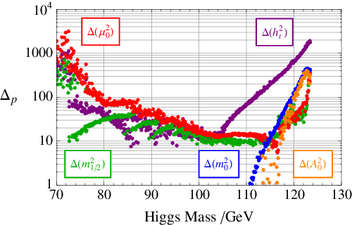
Turning now to the numerical results, Figure 1 presents the two-loop result for the dependence of overall electroweak fine tuning $\Delta$ as a function of the Higgs mass. The dark matter constraint and the LEPII bound on $m_{h}$ are not included. The loop effects reduce the fine tuning amount; the dominant effects come from quantum corrections to the quartic couplings (rather than to soft masses), which are increased by radiative effects and thus reduce $\Delta$ . $\Delta$ is seen to have a minimum close to the LEPII bound of $m_{h}$ . The individual contributions to $\Delta$ are shown in Figure 2. Below the LEPII bound, detailed calculations show that the minimal value of $\Delta$ is dominated by $\Delta_{\mu_{0}^{2}}$ and this increases rapidly for decreasing $m_{h}$ . For values of $m_{h}$ above the LEPII bound, $\Delta$ is dominated by⁵⁵ 5 Larger $m_{h}$ requires larger $m_{\tilde{t}}^{2}\sim m_{0}^{2}$ , and a larger $m_{0}$ , above the focus point region, increases $\Delta_{m_{0}^{2}}$ . $\Delta_{m_{0}^{2}}$ . This happens at the edge of the focus point region. The transition from the dominant $\Delta_{\mu_{0}^{2}}$ regime to the dominant $\Delta_{m_{0}^{2}}$ regime occurs near the LEPII bound value, and this is the point where the QCD radiative effects become important. This can be seen from Figure 1 where an increase by 1 $\sigma$ of $\alpha_{3}$ corresponds to a larger $\Delta$ for a same, fixed value of $m_{h}$ . In this sense one could even say that the minimal value of $\Delta$ is situated at the transition region between dominant effects, Yukawa versus QCD interactions. Away from the minimum of $\Delta$ , fine tuning increases dramatically, roughly exponentially. This is because, as discussed above, $\Delta$ depends exponentially on $m_{h}$ .

In conclusion, the fine tuning at two-loop with all the latest constraints is minimised for

\displaystyle\Delta\approx 8.8,\qquad m_{h}=114\pm 2\,\,\,\textrm{GeV}

(9)

with the theoretical uncertainty of $\pm 2$ GeV, explained earlier.

Note that our analysis also investigated the contribution to $\Delta$ coming from the uncertainty in measured ‘‘parameters’’ such as top Yukawa and strong coupling. Using the modified⁶⁶ 6 $\bar{\Delta}_{p}=\Delta_{p}\times(\sigma_{p}/p)$ where $\sigma_{p}$ is the 1 $\sigma$ error in the parameter $p$ derived from experimental observation. definition [26], appropriate for measured parameters, we find their fine-tuning is sub-dominant.

Finally, let us also mention that the reduction of fine-tuning that we have seen is mostly due to (two-) loop corrections considered, particularly to quartic couplings and is actually very significant, given the conservative scenario considered here assuming universal gaugino mass structure of the CMSSM; relaxing this condition could reduce [6] $\Delta$ further.

3.1 Constraints on $\Delta$ from fixing $\tan\beta$

It is interesting to examine the fine-tuning for fixed values of some of the parameters present, to see the individual impact of such constraints on $\Delta$ . Here we do this for a fixed value of $\tan\beta$ . This is shown⁷⁷ 7 In Figures 3, 4, 5 only, $\Delta$ is computed with our Mathematica code instead of SOFTSUSY, due to long CPU time constraints. This explains the small difference in shape between the two-loop line in these three figures from the more accurate one in Figure 1 and all other figures (based on SOFTSUSY). in Figure 3 for increasing vales of $\tan\beta$ , with $\tan\beta=2$ (blue), $\tan\beta=3$ (red), $\tan\beta=10$ (green). Increasing $\tan\beta$ shifts the curves of $\Delta$ towards larger $m_{h}$ and, to a limited extent, to lower fine-tuning, reached for medium $\tan\beta\sim 10$ , also for larger $\tan\beta\sim 40$ (see later, Fig.7 (a)). As may be seen from the figure, the two-loop expressions for soft masses and couplings bring values of $\Delta$ which are situated between the higher “tree-level” curve (i.e. tree-level for $\lambda_{i}$ , one-loop for soft masses without field dependent threshold effects) and the lower one-loop case (one-loop for both $\lambda_{i}$ and soft masses). This is consistent with what one would expect from a convergent, perturbative, loop expansion. The roughly exponential behaviour of $\Delta$ at large $m_{h}$ for fixed $\tan\beta$ can bring a significant variation of $\Delta$ .

3.2 Constraints on $\Delta$ from the SUSY spectrum

Here we examine the impact on $\Delta$ due to constraints related to the supersymmetric spectrum. The key features of the impact of this spectrum on $\Delta$ can be seen from the limits on the chargino mass considered in Figure 4. Currently, the (lightest) chargino mass bound is the most important, followed by that of the neutralino. It also turns out that the gluino mass limit is not very constraining. These results follow recent experimental data, since using the 1998 data it was the neutralino mass bound that was more constraining for $\Delta$ .

In Figure 4, the effect of the chargino mass $m_{\chi_{1}}>94$ and $m_{\chi_{1}}>80$ GeV is shown by the upper and lower continuous curves. While these can have some impact on fine-tuning for values of $m_{h}$ already ruled out experimentally, for $m_{h}>114.4$ GeV, the effect is overlapping that from $b\rightarrow s\gamma$ (see later). Further, the close vicinity of the upper and lower dotted curves corresponding to all constraints in Table 1 and to the SUSY spectrum limits respectively shows that the latter are the main constraints at the moment for $\Delta$ at low $\tan\beta$ . The graph presents $\Delta$ and $m_{h}$ computed using quartic couplings and mass expressions evaluated at two-loop.

3.3 Constraints on $\Delta$ from $b\rightarrow s\gamma$

Figure 5 gives the impact of the $b\rightarrow s\gamma$ constraint on $\Delta$ . The lower limit of the $b\to s\gamma$ constraint for a given coloured area (fixed $\tan\beta$ ) restricts the right hand edges of the plot, while the upper limit restricts its left hand side. These curves also depend on the mass limits - these constraints are not fully independent. For the experimentally allowed area of $m_{h}>114.4$ GeV, the impact of the constraint $b\rightarrow s\gamma$ is rather small; in this case its effect is overlapping that of the SUSY mass limits, as can be seen from the rhs of the plots for individual $\tan\beta$ plots. The combination of the SUSY mass limits and $b\rightarrow s\gamma$ constraint currently dominate the restriction on how small the fine tuning could be, see also Figure 6. In this last figure one can easily see, at two-loop, the impact on $\Delta$ of removing the $b\rightarrow s\gamma$ constraint. For a related analysis of $b\rightarrow s\gamma$ see recent [27].

The other constraints listed in Table 1 do eliminate further mSUGRA points, but have a negligible effect on the fine tuning limits. With the current mass limits, a change in the $\delta a_{\mu}$ constraint by factors of 2 or more does not affect these results significantly.

3.4 Constraints on $\Delta$ and the CMSSM parameters

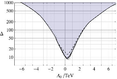
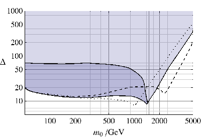
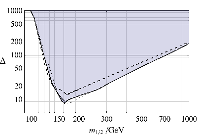
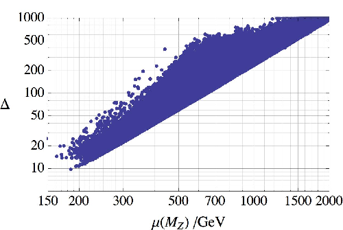
The fine tuning measure can be easily applied to establish the remaining allowed range for the MSSM SUSY parameters. In Figure 7 we plotted the dependence of the total fine tuning wrt various parameters. To understand some aspects of the dependence of the electroweak scale fine tuning on the MSSM parameters, let us use, for the sake of discussion, one of the two minimum conditions which, when ignoring quantum corrections to quartic couplings, simplifies to:

\displaystyle\frac{m_{Z}^{2}}{2}

\displaystyle=

\displaystyle\frac{{m}_{1}^{2}-{m}_{2}^{2}\tan^{2}\beta}{\tan^{2}\beta-1}

(10)

Using 2-loop RGE solutions at $\tan\beta=10$ (for details see the Appendix), one has

	$\displaystyle{m}_{1}^{2}\,(m_{Z})$	$\displaystyle\approx$	$\displaystyle 0.99\,\mu_{0}^{2}+0.946\,m_{0}^{2}+0.331\,m_{1/2}^{2}+0.044\,A_{0}\,m_{1/2}-0.013\,A_{0}^{2}$		(11)
	$\displaystyle{m}_{2}^{2}\,(m_{Z})$	$\displaystyle\approx$	$\displaystyle 0.99\,\mu_{0}^{2}-0.080\,m_{0}^{2}-2.865\,m_{1/2}^{2}+0.445\,A_{0}\,m_{1/2}-0.099\,A_{0}^{2}$		(12)

It is the large cancellation between the $\mu_{0}^{2}$ and $m_{1/2}^{2}$ terms that is often responsible for the large fine tuning (note however that this argument ignores the impact of quantum corrections to quartic couplings, known to reduce the fine-tuning). This leads to the approximate relation $\Delta_{\mu_{0}^{2}}\sim\Delta_{m_{1/2}^{2}}$ . As low fine tuning prefers small $\mu_{0}$ , small $m_{1/2}$ is also preferred and this is observed in Fig 7 (e), (f). The rise in fine tuning at small $m_{1/2}$ is a consequence of the constraints such as the chargino mass limit.

The near flat distribution of minimum fine tuning in $m_{0}$ is a result of the coefficient of $m_{0}$ in $m_{2}$ being driven close to zero. The fine tuning with respect to $m_{0}$ then rarely dominates, until we reach values of $m_{h}$ above the LEPII bound ( $m_{0}$ at the edge of focus point region). The result of applying the Higgs mass constraint also excludes a region with small $m_{1/2}$ at $m_{0}$ below 1.5 TeV. The focus point at $m_{0}\sim 1.5$ TeV where the minimum of $m_{1/2}$ is possible, corresponds to the point where fine tuning is minimised. This only occurs for large $\tan\beta$ , and this available “dip” in fine tuning in the mSUGRA space disappears as $\tan\beta$ is reduced.

Figure 7(c) indicates that a small trilinear coupling $|A_{0}|\lesssim 1$ TeV is preferred for the smallest fine tuning. This follows from a similar argument for preferring small $m_{1/2}$ . Increasing $|A_{0}|$ requires larger cancellations with $\mu$ to set the electroweak scale. However, once the Higgs mass constraint is applied, $A_{0}$ is driven negative for small $\tan\beta$ in order to maximise the stop mixing. The related increase in the minimum fine tuning from being in this region of parameter space then follows. This is important for small $\tan\beta$ where the tree level Higgs mass is smallest. The sign structure of the UV parameter coefficients in $m_{2}$ leads to a preference in a small, positive $A_{0}$ .

As mentioned earlier, the fine tuning measure $\Delta$ can be used to establish the remaining parameter space of the CMSSM compatible with a solution to the hierarchy problem. Assuming that $\Delta=100$ is the upper limit beyond which we consider that SUSY failed to solve the hierarchy problem, we obtain the following bounds:

$m_{h}$	$<~121$ GeV		$5.5~<$	$\tan\beta$	$<~55$
$\mu$	$<~680$ GeV		120 GeV $~<$	$m_{1/2}$	$<~720$ GeV
$m_{0}$	$<~3.2$ TeV		$-2.0$ TeV $~<$	$A_{0}$	$<~2.5$ TeV

(13)

These values can be easily re-calculated for a different value of $\Delta$ .

3.5 Constraints on $\Delta$ from the relic density

It is interesting to see the impact on $\Delta$ and on the CMSSM parameters from the presence of the dark matter relic density constraint (examined using micrOMEGAs2.2 [35]) and the LEPII constraint on $m_{h}$ . These are rather strong constraints, particularly in the “restrictive” context of CMSSM that we study, with universal gaugino mass. The results are presented in Figure 8, where the relative impact of the LEPII constraint can be seen by comparing the left and right plots. If the observed dark matter abundance is imposed as a constraint on the CMSSM, then the range of values given in (13) and valid for $\Delta<100$ is further restricted, as seen in Figure 8. The condition that the SUSY LSP should provide the observed dark matter abundance as well as the constraint $m_{h}>114.4$ GeV removes the intermediate values of $m_{1/2}$ and $m_{0}$ , but has a rather small impact on $A_{0}$ .

3.6 Prediction for $m_{h}$ from minimising $\Delta$ and saturating the relic density

The relic density constraint can be combined with that of minimal electroweak fine-tuning $\Delta$ to make an interesting prediction for $m_{h}$ . Figure 9 shows the impact of non-baryonic relic density constraint on $\Delta$ presented in Figure 1. Obviously, not all initial points in $\Delta$ satisfy this constraint, and this is shown in Figure 9 by the red and blue points which do not fill the whole area above the continuous line of minimal $\Delta$ . As expected, the additional dark matter constraint prefers in some cases larger $\Delta$ relative to its minimal value (continuous line) obtained only with the constraints in Table 1. However, as can be seen in the plots, the region of $m_{h}$ values where this constraint is indeed relevant is actually ruled out by LEPII bound $m_{h}>114.4$ GeV; above this value the two curves on the boundary are almost overlapped and the constraints in Table 1 are sufficient to also satisfy the thermal relic density; note that the red points in the left (right) plots in Figure 9 satisfy the relic density within 1 $\sigma$ and 3 $\sigma$ WMAP bounds [33], respectively. The results are obtained as usual, using two-loop values for the quartic couplings and soft masses and corresponding threshold effects. (with the SOFTSUSY and micrOMEGAs codes).

It is important to notice that, without imposing the LEPII bound, at the two-loop level, the smallest fine tuning $\Delta$ consistent with the relic density WMAP bounds [33] predicts a mass for the lightest Higgs as follows:

$\displaystyle m_{h}$	$\displaystyle=$	$\displaystyle 114.7\pm 2\,\,\,\mbox{GeV},\,\,\,\,\,\Delta=15.0,\,\,\,\,\,\textrm{(sub-saturating the WMAP bound).}$
$\displaystyle m_{h}$	$\displaystyle=$	$\displaystyle 116.0\pm 2\,\,\,\mbox{GeV},\,\,\,\,\,\Delta=19.1,\,\,\,\,\,\textrm{(saturating the WMAP within 1$\sigma$).}$
$\displaystyle m_{h}$	$\displaystyle=$	$\displaystyle 115.9\pm 2\,\,\,\mbox{GeV},\,\,\,\,\,\Delta=17.8,\,\,\,\,\,\textrm{(saturating the WMAP within 3$\sigma$).}$	(14)

To conclude, minimising the fine-tuning together with the constraints from precision electroweak data, the bounds on SUSY masses and the requirement of the observed dark matter abundance lead to a prediction for $m_{h}$ , without imposing the LEPII bound. This is an interesting result, and represents our prediction for the CMSSM lightest Higgs mass based on assuming $\Delta$ as a quantitative test of SUSY as a solution to the hierarchy problem.

4 Dark matter fine tuning and its effect on the Higgs mass

The dark matter abundance can be very sensitive to the choice of parameters and can introduce a new fine tuning to the model. To quantify this it is interesting to consider the dark matter fine tuning $\Delta^{\Omega}$ wrt the CMSSM parameters, and to determine its impact on the overall fine tuning (for earlier studies see [15, 16] and references therein). Its definition is similar to that of $\Delta$ :

\displaystyle\Delta^{\Omega}=\max\bigg|\frac{\partial\ln\Omega h^{2}}{\partial\ln q}\bigg|_{q=m_{0},m_{1/2},A_{0},\tan\beta}

(15)

In Figure 10 we evaluated $\Delta^{\Omega}$ at two-loop level and presented as a function of the Higgs mass, without imposing any restriction on the latter. It turns out that $\Delta^{\Omega}$ can have acceptable values even for $m_{h}$ close to $120$ GeV. In Figure 11 the total fine-tuning, defined as $\max\{\Delta,\Delta^{\Omega}\}$ is presented as a function of $m_{h}$ . Its value is only slightly larger than that found earlier for $\Delta$ alone with WMAP saturated dark matter abundance (in red in the plots). From Figure 11 we predict, from minimising $\max\{\Delta,\Delta^{\Omega}\}$ and from consistency with the 3 $\sigma$ WMAP bound:

	$\displaystyle m_{h}$	$\displaystyle=$	$\displaystyle\!\!114.70\pm 2\,\,\mbox{GeV},\,\,\max\{\Delta,\Delta^{\Omega}\}=15,\,\,\,\,\,\,\textrm{(sub-saturating WMAP bound)}$
	$\displaystyle m_{h}$	$\displaystyle=$	$\displaystyle\!\!116.98\pm 2\,\,\mbox{GeV},\,\,\max\{\Delta,\Delta^{\Omega}\}=28.7,\,\,\,\textrm{(saturating WMAP bound within 3$\sigma$)\,\,\,\,\,\,}$		(16)

The last predicted value of $m_{h}$ is only marginally above that predicted in (14), based on minimised electroweak fine-tuning and right dark matter abundance.

5 Predictions for the superpartners from fine tuning limits

The results so far demonstrate that electroweak fine-tuning has a strong sensitivity to parameters such as $\mu$ , $m_{1/2}$ , with a preference for lower values. Regarding the $m_{0}$ dependence, $\Delta$ has a rather flat dependence when we are in the focus point region. The states that are dominantly controlled by the $\mu$ , $m_{1/2}$ parameters are then the most important in determining the naturalness of the proposed theory. These include the neutralinos, charginos and the gluino states. Further, setting an upper bound on electroweak $\Delta$ gives a bound on the spectrum. If any of these states have masses in excess of those given in Table 2, it will require less than 1% tuning ( $\Delta>100$ ) for the MSSM.

$\tilde{g}$	$\chi_{1}^{0}$	$\chi_{2}^{0}$	$\chi_{3}^{0}$	$\chi_{4}^{0}$	$\chi_{1}^{\pm}$	$\chi_{2}^{\pm}$	$\tilde{t}_{1}$	$\tilde{t}_{2}$	$\tilde{b}_{1}$	$\tilde{b}_{2}$
1720	305	550	660	665	550	670	2080	2660	2660	3140

Table 2: Upper mass limits on superpartners in GeV such that

\Delta<100

remains possible.

These upper mass limits scale approximately as $\sqrt{\Delta_{\mbox{\tiny min}}}$ , so they may be adapted depending on how much fine tuning the reader is willing to accept. Overall low fine tuning prefers a Higgsino mass of ${\cal O}(0.5~\textrm{TeV})$ , a gluino of ${\cal O}(1.5~\textrm{TeV})$ and chargino and neutralino masses of ${\cal O}(300~\textrm{GeV})$ . Stop and sbottom masses are significantly larger at ${\cal O}(3~\textrm{TeV})$ due to the weak limit on $m_{0}$ (focus point).

Finally we return to the intriguing fact that minimum electroweak fine tuning plus correct dark matter abundance corresponds to a Higgs mass just above the LEPII bound⁸⁸ 8 One may ask whether the fine-tuning measure used above has indeed a clear physical meaning. One can object that nature may not choose “minimal” fine-tuning results. One can invoke the example of classical chaotic systems, displaying the familiar “butterfly effect” where small variations of the initial conditions bring large changes of the final state (“fine tuning”), yet the system is “realised”. Such effects exist in (nonlinear) classical systems, where initial close values (states) of a parameter exponentially diverge after evolving according to the dynamics of the differential eqs. In our setup, one could have such effects not from evolution in time but from evolution wrt the energy scale, from the high scale to the low scale, after including quantum effects encoded in the RG differential equations. By this analogy one could object that using criteria of low fine-tuning to obtain mass bounds (for $m_{h}$ ) may not be appropriate. However, the difference is that the discussion in the text is at quantum level, so the counterexamples of classical (chaotic) systems do not necessarily apply.. As we noted above this point is fixed by the current bounds on the SUSY spectrum and not by the current Higgs mass bound which is not included when doing the scans giving Figs 1, 2, 9, 11.

One may interpret the SUSY parameters corresponding to this point as being the most likely given our present knowledge and so it is of interest to compute the SUSY spectrum for this parameter choice as a benchmark for future searches. This is presented in Table 3 where it may be seen that it is somewhat non-standard with very heavy squarks and sleptons and lighter neutralinos, charginos and gluinos. This has similarities to the SPS2 scenario [36].

$h^{0}$	114.5	$\tilde{\chi}_{1}^{0}$	79	$\tilde{b}_{1}$	1147	$\tilde{u}_{L}$	1444
$H^{0}$	1264	$\tilde{\chi}_{2}^{0}$	142	$\tilde{b}_{2}$	1369	$\tilde{u}_{R}$	1446
$H^{\pm}$	1267	$\tilde{\chi}_{3}^{0}$	255	$\tilde{\tau}_{1}$	1328	$\tilde{d}_{L}$	1448
$A^{0}$	1264	$\tilde{\chi}_{4}^{0}$	280	$\tilde{\tau}_{2}$	1368	$\tilde{d}_{R}$	1446
$\tilde{g}$	549	$\tilde{\chi}_{1}^{\pm}$	142	$\tilde{\mu}_{L}$	1406	$\tilde{s}_{L}$	1448
$\tilde{\nu}_{\tau}$	1366	$\tilde{\chi}_{2}^{\pm}$	280	$\tilde{\mu}_{R}$	1406	$\tilde{s}_{R}$	1446
$\tilde{\nu}_{\mu}$	1404	$\tilde{t}_{1}$	873	$\tilde{e}_{L}$	1406	$\tilde{c}_{L}$	1444
$\tilde{\nu}_{e}$	1404	$\tilde{t}_{2}$	1158	$\tilde{e}_{R}$	1406	$\tilde{c}_{R}$	1446

Table 3: The favoured Constrained MSSM spectrum of minimal

\Delta=15

giving a sub-saturation of the WMAP bound. Masses are given in

GeV

5.1 Predictions for SUSY searches at the LHC

It is clear that there is still a wide range of parameters that needs to be explored when testing the CMSSM. Will the LHC be able to cover the whole range? To answer this note that, for a fine tuning measure $\Delta<100$ , one must be able to exclude the upper limits of the mass parameters appearing in Table 2. Of course the state that affects fine tuning most is the Higgs scalar and one may see from Figure 1 that establishing the bound $m_{h}>120$ GeV will imply that $\Delta>100.$ However the least fine tuned region corresponds to the lightest Higgs consistent with the LEPII bound and this is the region where the LHC searches rely on the $h\rightarrow\gamma\gamma$ channel which has a small cross section and will require some $30\,fb^{-1}$ at $\sqrt{s}=14$ TeV to explore. Given this it is of interest to consider to what extent the direct SUSY searches will probe the low fine tuned regions. Following the discussion in the previous section, the most significant processes at the LHC will be those looking for gluinos, winos and neutralinos.

Studies of SUSY at the LHC [37] have shown that the LHC experiments have a sensitivity to gluinos of mass $1.9$ TeV for $\sqrt{s}=10$ TeV, $2.4$ TeV for $\sqrt{s}=14$ TeV and luminosity $10fb^{-1}.$ Of relevance to the first LHC run the limit is $600$ GeV for $\sqrt{s}=10$ TeV and luminosity $100\,pb^{-1}.$ These correspond to probing up to $\Delta=120,180$ and $14$ respectively. As we have discussed charginos and neutralinos can be quite light, but their signal events are difficult for LHC to extract from the background, owing in part to a decreasing $M_{\widetilde{W}}-M_{\widetilde{Z}}$ mass gap as $\left|\mu\right|$ decreases [38, 39]. An Atlas study [40] of the trilepton signal from chargino-neutralino production found that $30fb^{-1}$ luminosity at 14 TeV is needed for a 3 $\sigma$ discovery significance for $M_{2}<300$ GeV and $\mu<250$ GeV [41].

6 Summary and Conclusions

Supersymmetry was introduced to solve the hierarchy problem and to avoid the large fine-tuning in the SM Higgs sector associated with the Planck or GUT scale when quantum corrections are included. While this hierarchy problem is solved by TeV-scale supersymmetry, the non-observation, so far, of SUSY states means that the MSSM has acquired some residual amount of fine-tuning related to unnatural cancellations in the SUSY breaking sector. The goal of this paper was to analyse in detail the level of fine tuning in the CMSSM.

The fine tuning measure $\Delta$ provides a quantitative test of SUSY as a solution to the “little” hierarchy problem and measures the “tension” required to satisfy the scalar potential minimum condition $v^{2}\sim-m_{susy}^{2}/\lambda$ , for a combination of soft masses $m_{susy}^{2}\sim$ TeV, with an effective quartic coupling $\lambda<1$ and $v\sim{\cal O}(100)$ GeV. Although the exact upper limit on the fine tuning $\Delta$ beyond which a theory fails to solve the hierarchy problem is debatable, it is preferable, for a given model, to have a parameter space configuration corresponding to the lowest value of $\Delta$ . We evaluated $\Delta$ at two-loop order and also paid particular attention to threshold corrections and to the $\tan\beta$ radiative dependence on the parameters. Such effects on fine-tuning were not fully considered in the past and turned out to reduce fine tuning significantly.

Our determination of the fine-tuning measure for the CMSSM included the theoretical constraints (radiative EWSB, avoiding charge and colour breaking vacua), and also the experimental constraints (bounds on superpartner masses, electroweak precision data, $b\rightarrow s\,\gamma$ , $b\rightarrow\mu\,\mu$ and muon anomalous magnetic moment, dark matter abundance). As far as we are aware, our study is the first two-loop analysis of the fine tuning problem in the CMSSM, largely based on SOFTSUSY and micrOMEGAs, SuSpect and our own Mathematica code. The latter was very important since it reduced to a feasible level the CPU run time necessary to scan the full parameter space.

Not including the dark matter constraint, we found the minimum value is given by $\Delta=8.8$ . Remarkably, even without imposing the LEP bound on the Higgs mass, the condition fine tuning should be a minimum predicts $m_{h}=114\pm 2$ GeV. Adding the constraint on the dark matter relic density, one finds $\Delta=15$ corresponding to $m_{h}=114.7\pm 2$ GeV and this rises to $\Delta=17.8$ ( $m_{h}=115.9\pm 2$ GeV) for SUSY dark matter abundance within 3 $\sigma$ of the WMAP constraint. The results are encouraging for the search for SUSY because we considered the “conservative” case of CMSSM, and it is well-known that relaxing gaugino universality can reduce $\Delta$ further [6, 9].

The spectrum corresponding to the minimum value of the fine tuning shows similarities to the SPS2 scenario with light neutralinos, charginos and gluinos (corresponding to light $\mu$ , $m_{1/2}$ ) and heavy squarks and sleptons corresponding to large $m_{0}$ , near the focus point limiting value [13, 14]. It provides the ”best” estimate for the SUSY spectrum given the present experimental bounds.

Increasing $m_{h}$ above the minimum fine tuned value causes $\Delta$ to increases exponentially fast and one leaves the focus point region at the edge of which this minimal value is reached; one obtains $\Delta~\!=~\!100\,\,(1000)$ for a scalar mass $m_{h}=121$ ( $126$ ) GeV, respectively. Ultimately the question whether the SUSY solution to the hierarchy problem has been experimentally tested relies on what value of fine tuning represents the limit of acceptability. Given a value one can determine the range of parameter space that is still acceptable. For the case that the fine tuning measure should satisfy $\Delta<100$ , we determined the corresponding superpartners masses and CMSSM parameters values, that can be relevant for SUSY searches.

Acknowledgements

The research was partially supported by the EU RTN grant UNILHC 23792. S.C. is supported by the UK Science and Technology Facilities Council PPA/S/S/2006/04503. D.G. thanks the Theory Group at École Polytechnique Paris for their kind hospitality and acknowledges the financial support from the ERC Advanced Grant ERC-2008-AdG 20080228 (“MassTeV”). D.G. thanks S. Pokorski for many interesting discussions on this topic.

7 Appendix

A.1 Higgs mass and EW fine tuning

We provide technical results used in the text to evaluate $\Delta$ . The potential used in (1)

$\displaystyle V$	$\displaystyle=$	$\displaystyle m_{1}^{2}\,\,\|H_{1}\|^{2}+m_{2}^{2}\,\,\|H_{2}\|^{2}-(m_{3}^{2}\,\,H_{1}\cdot H_{2}+h.c.)$	(A-1)
		$\displaystyle~+~\frac{1}{2}\,\lambda_{1}\,\|H_{1}\|^{4}+\frac{1}{2}\,\lambda_{2}\,\|H_{2}\|^{4}+\lambda_{3}\,\|H_{1}\|^{2}\,\|H_{2}\|^{2}\,+\lambda_{4}\,\|H_{1}\cdot H_{2}\|^{2}$
		$\displaystyle~+~\bigg[\,\frac{1}{2}\,\lambda_{5}\,\,(H_{1}\cdot H_{2})^{2}+\lambda_{6}\,\,\|H_{1}\|^{2}\,(H_{1}\cdot H_{2})+\lambda_{7}\,\,\|H_{2}\|^{2}\,(H_{1}\cdot H_{2})+h.c.\bigg]$

with $H_{1}.H_{2}=H_{1}^{0}\,H_{2}^{0}-H_{1}^{-}H_{2}^{+}$ . Using the notation

	$\displaystyle m^{2}$	$\displaystyle=$	$\displaystyle m_{1}^{2}\,\cos^{2}\beta+m_{2}^{2}\,\sin^{2}\beta-m_{3}^{2}\,\sin 2\beta$
	$\displaystyle\lambda$	$\displaystyle=$	$\displaystyle\frac{\lambda_{1}}{2}\,\cos^{4}\beta+\frac{\lambda_{2}}{2}\,\sin^{4}\beta+\frac{\lambda_{345}}{4}\,\sin^{2}2\beta+\sin 2\beta\left(\lambda_{6}\cos^{2}\beta+\lambda_{7}\sin^{2}\beta\right)$		(A-2)

the minimisation conditions give

\displaystyle v^{2}=-m^{2}/\lambda,\qquad 2\lambda\frac{\partial m^{2}}{\partial\beta}=m^{2}\frac{\partial\lambda}{\partial\beta}

(A-3)

or, equivalently,

	$\displaystyle\frac{2m_{3}^{2}}{\sin 2\beta}~=~m_{1}^{2}+m_{2}^{2}+\frac{v^{2}}{2}\left[\lambda_{1}\,c^{2}_{\beta}+\lambda_{2}\,s^{2}_{\beta}+\lambda_{345}+\left(\lambda_{6}+\lambda_{7}\right)s_{2\beta}+\lambda_{6}\cot\beta+\lambda_{7}\tan\beta\right]$
	$\displaystyle m_{1}^{2}-m_{2}^{2}\tan^{2}\beta~=~-\frac{v^{2}}{2}\left[\cos^{2}\beta\left(\lambda_{1}-\lambda_{2}\tan^{4}\beta\right)+\sin 2\beta\left(\lambda_{6}-\lambda_{7}\tan^{2}\beta\right)\right]$		(A-4)

One finds for the CP odd Higgs mass:

\displaystyle m_{A}^{2}

\displaystyle=

\displaystyle\frac{2m_{3}^{2}}{\sin 2\beta}-\frac{v^{2}}{2}\,\left(2\lambda_{5}+\lambda_{6}\cot\beta+\lambda_{7}\tan\beta\right),\hskip 28.45274ptm_{Z}^{2}~=~\frac{g^{2}\,v^{2}}{4}

(A-5)

with $g^{2}=g_{1}^{2}+g^{2}_{2}$ . In the notation of [42], the CP even Higgs masses are

$\displaystyle m_{h}^{2}$	$\displaystyle=$	$\displaystyle\frac{1}{2}\Big[\,m_{A}^{2}+v^{2}\left(2\lambda+\Lambda_{5}\right)-\sqrt{\left[m_{A}^{2}+v^{2}\left(\Lambda_{5}-2\lambda\right)\right]^{2}+4v^{4}\,\Lambda_{6}^{2}\,}\,\Big]$
$\displaystyle\Lambda_{5}$	$\displaystyle=$	$\displaystyle\frac{s^{2}_{2\beta}}{4}\,\left(\lambda_{1}+\lambda_{2}-2\lambda_{345}\right)+\lambda_{5}-\frac{s_{4\beta}}{2}\,(\lambda_{6}-\lambda_{7})$
$\displaystyle\Lambda_{6}$	$\displaystyle=$	$\displaystyle\frac{s_{2\beta}}{2}\left(\lambda_{3451}\,c^{2}_{\beta}-\lambda_{3452}\,s^{2}_{\beta}\right)+\frac{c_{2\beta}}{2}\left(\lambda_{6}+\lambda_{7}\right)+\frac{c_{4\beta}}{2}\left(\lambda_{6}-\lambda_{7}\right)$	(A-6)

where $\lambda_{345j}=\lambda_{345}-\lambda_{j}$ , $\lambda$ is that of (2), and, $(s_{\beta},c_{\beta})=(\sin\beta,\cos\beta)$ . In the limit of large $m_{A}$ , $m_{h}^{2}$ reaches an upper limit of $2\lambda v^{2}$ (which tends to $\lambda_{2}v^{2}$ for large $\tan\beta$ ). At tree level, $\lambda=(g^{2}/8)\cos^{2}2\beta$ , and the individual $\lambda_{j}$ are:

\displaystyle\lambda_{1,2}~=\,-\lambda_{345}~=~\frac{g^{2}}{4}\hskip 42.67912pt\lambda_{5,6,7}~=~0

(A-7)

The general formula for fine-tuning $\Delta_{p}$ wrt a parameter $p$ in a two-higgs doublet model that we are using can be found in the Appendix of [17]. For large $\tan\beta=v_{2}/v_{1}$ this reduces to

$\displaystyle\Delta_{p}$	$\displaystyle=$	$\displaystyle\frac{\partial\ln v^{2}}{\partial\ln p}$	(A-8)
	$\displaystyle=$	$\displaystyle\frac{[4\lambda_{7}\,(m_{3}^{2})^{\prime}-4\lambda_{7}^{\prime}\,m_{3}^{2}]+[\lambda_{2}^{\prime}\,v^{2}+2(m_{2}^{2})^{\prime}]\,[\lambda_{3452}+2(m_{1}^{2}-m_{2}^{2})/v^{2}]}{2\lambda_{7}^{2}\,v^{2}-\lambda_{2}\,[\lambda_{3452}\,\,v^{2}+2\,(m_{1}^{2}-m_{2}^{2})]}+{\mathcal{O}}(\cot\beta)$
	$\displaystyle\rightarrow$	$\displaystyle-\frac{1}{\lambda_{2}\,v^{2}}\left[2\,(m_{2}^{2})^{\prime}+\lambda_{2}^{\prime}\,v^{2}+4\,v^{2}\left(\frac{\lambda_{7}\,(m_{3}^{2})^{\prime}-\lambda_{7}^{\prime}\,m_{3}^{2}}{\lambda_{3452}\,\,v^{2}+2\,(m_{1}^{2}-m_{2}^{2})}\right)\right],\,\,\,(\textrm{if}\,\,\lambda_{7}\|\ll\|\lambda_{2}\|,\|\lambda_{3452}\|)$

where $x^{\prime}=\partial x/\partial\ln p$ is the partial derivative of $x$ wrt $p$ .

A.2 The scalar potential: 1 Loop Leading Log (1LLL) Terms

Here we show how to obtain the one-loop corrected potential, which is “improved” to the two-loop leading log (2LLL) result in the next section. Start with

\displaystyle V^{(0)}

\displaystyle=

\displaystyle\bar{m}_{1}^{2}\left|H_{1}\right|^{2}+\bar{m}_{2}^{2}\left|H_{2}\right|^{2}-\bar{m}_{3}^{2}\left(H_{1}H_{2}+\mbox{h.c.}\right)+\frac{g^{2}}{8}\left(\left|H_{1}\right|^{2}-\left|H_{2}\right|^{2}\right)^{2}

(A-9)

This receives (field dependent threshold) corrections, computed using the Coleman-Weinberg potential [43]:

\displaystyle V^{(1)}

\displaystyle=

\displaystyle\frac{1}{64\pi^{2}}\,\sum_{k}\,(-1)^{2J_{k}}\,(2J_{k}+1)\,g_{k}\,m_{k}^{4}\left(\log\frac{m_{k}^{2}}{Q^{2}}-\frac{3}{2}\right)

(A-10)

where $m_{k}$ is the field dependent mass, the degeneracy factor $g_{k}$ is 6 for squarks, and $J_{k}$ is the particle spin. All parameters in eq.(A-10) are evaluated at the scale Q using the RGEs which ignore the particle masses. The field dependent squark masses are (neglecting $O\!\left(g^{4}\right)$ terms):

	$\displaystyle m_{\tilde{t}_{1,2}}^{2}$	$\displaystyle\approx$	$\displaystyle M_{S}^{2}+h_{t}^{2}\left\|H_{2}\right\|^{2}+\frac{g^{2}}{8}\left(\left\|H_{1}\right\|^{2}-\left\|H_{2}\right\|^{2}\right)\mp h_{t}\left\|A_{t}H_{2}-\mu H_{1}^{*}\right\|$		(A-11)
	$\displaystyle m_{\tilde{b}_{1,2}}^{2}$	$\displaystyle\approx$	$\displaystyle M_{S}^{2}+h_{b}^{2}\left\|H_{1}\right\|^{2}+\frac{g^{2}}{8}\left(\left\|H_{2}\right\|^{2}-\left\|H_{1}\right\|^{2}\right)\mp h_{b}\left\|A_{b}H_{1}-\mu H_{2}^{*}\right\|$		(A-12)

and where $m_{Q,U,D}(M_{S})=M_{S}$ is assumed. Here, $M_{S}$ is the soft SUSY breaking squark mass evaluated at the squark mass scale.

One can expand the non-linear field dependence (log) in $V^{(1)}$ in inverse powers of $1/M_{S}$ to find the dominant threshold corrections, which come from the third generation squarks:

$\displaystyle V^{(1)}_{\tilde{t}_{1,2}}$	$\displaystyle\approx$	$\displaystyle\frac{3}{16\pi^{2}}\Bigg[t\left(h_{t}^{4}\left\|H_{2}\right\|^{4}+2h_{t}^{2}\,M_{S}^{2}\left\|H_{2}\right\|^{2}+h_{t}^{2}\left\|A_{t}H_{2}-\mu H_{1}^{*}\right\|^{2}\right)$	(A-13)
		$\displaystyle\hskip 42.67912pt+~h_{t}^{4}~\frac{\left\|A_{t}H_{2}-\mu H_{1}^{}\right\|^{2}}{M_{S}^{2}}\left(\left\|H_{2}\right\|^{2}-\frac{\left\|A_{t}H_{2}-\mu H_{1}^{}\right\|^{2}}{12M_{S}^{2}}\right)$
		$\displaystyle\hskip 14.22636pt+~\frac{g^{2}}{8}\left(\left\|H_{1}\right\|^{2}-\left\|H_{2}\right\|^{2}\right)\left(2t\,h_{t}^{2}\left\|H_{2}\right\|^{2}+2M_{S}^{2}\left(t-1\right)+\frac{\left\|A_{t}H_{2}-\mu H_{1}^{*}\right\|^{2}}{M_{S}^{2}}\right)\Bigg]\qquad$

$\displaystyle V^{(1)}_{\tilde{b}_{1,2}}$	$\displaystyle\approx$	$\displaystyle\frac{3}{16\pi^{2}}\Bigg[t\left(h_{b}^{4}\left\|H_{1}\right\|^{4}+2h_{b}^{2}\,M_{S}^{2}\left\|H_{1}\right\|^{2}+h_{b}^{2}\left\|A_{b}H_{1}-\mu H_{2}^{*}\right\|^{2}\right)$	(A-14)
		$\displaystyle\hskip 42.67912pt+~h_{b}^{4}~\frac{\left\|A_{b}H_{1}-\mu H_{2}^{}\right\|^{2}}{M_{S}^{2}}\left(\left\|H_{1}\right\|^{2}-\frac{\left\|A_{b}H_{1}-\mu H_{2}^{}\right\|^{2}}{12M_{S}^{2}}\right)$
		$\displaystyle\hskip 14.22636pt+~\frac{g^{2}}{8}\left(\left\|H_{2}\right\|^{2}-\left\|H_{1}\right\|^{2}\right)\left(2t\,h_{b}^{2}\left\|H_{1}\right\|^{2}+2M_{S}^{2}\left(t-1\right)+\frac{\left\|A_{b}H_{1}-\mu H_{2}^{*}\right\|^{2}}{M_{S}^{2}}\right)\Bigg]\qquad$

where

\displaystyle t=\log(M_{S}^{2}/Q^{2})

(A-15)

When running below the EWSB scale, the inclusion of higher dimensional terms (threshold corrections) lead to a re-summation such that $M_{S}$ is replaced by a mass scale related to the physical particle masses [44]. For the results of this paper, the geometric mean of the stop masses is used in the place of $M_{S}$ .

The above equations are valid down to the top mass scale; below this scale threshold corrections from the top quark should also be included. The dominant effect of running below the top scale can be absorbed by setting $Q$ in the above equations as the “running” top mass evaluated at the scale $Q$ instead of the pole mass.

From eqs.(A-9) to (A-14) one obtains the parameters entering in the scalar potential (1), evaluated at the scale Q (below $M_{S}$ ), in the one-loop leading log approximation (1LLL):

$\displaystyle m_{1}^{2}$	$\displaystyle=$	$\displaystyle\bar{m}_{1}^{2}-\frac{6h_{b}^{2}}{16\pi^{2}}\,M_{S}^{2}+\frac{3}{16\pi^{2}}\left(2h_{b}^{2}\,M_{S}^{2}+h_{b}^{2}A_{b}^{2}+h_{t}^{2}\mu^{2}\right)t$	(A-16)
$\displaystyle m_{2}^{2}$	$\displaystyle=$	$\displaystyle\bar{m}_{2}^{2}-\frac{6h_{t}^{2}}{16\pi^{2}}\,M_{S}^{2}+\frac{3}{16\pi^{2}}\left(2h_{t}^{2}\,M_{S}^{2}+h_{t}^{2}A_{t}^{2}+h_{b}^{2}\mu^{2}\right)t$	(A-17)
$\displaystyle m_{3}^{2}$	$\displaystyle=$	$\displaystyle\bar{m}_{3}^{2}+\frac{3}{16\pi^{2}}\left(h_{t}^{2}A_{t}+h_{b}^{2}A_{b}\right)\mu\,t$	(A-18)

	$\displaystyle\lambda_{1}$	$\displaystyle=$	$\displaystyle\frac{g^{2}}{4}\left(1+\frac{3\left(h_{t}^{2}\,\mu^{2}-h_{b}^{2}\,A_{b}^{2}\right)}{16\pi^{2}\,M_{S}^{2}}\right)+\frac{3}{8\pi^{2}}\left(\frac{h_{b}^{4}\,X_{b}}{2}-\frac{h_{t}^{4}\,\mu^{4}}{12M_{S}^{4}}\right)+\frac{3h_{b}^{2}}{8\pi^{2}}\left(h_{b}^{2}-\frac{g^{2}}{4}\right)t\hskip 28.45274pt$		(A-19)
	$\displaystyle\lambda_{2}$	$\displaystyle=$	$\displaystyle\frac{g^{2}}{4}\left(1+\frac{3\left(h_{b}^{2}\,\mu^{2}-h_{t}^{2}\,A_{t}^{2}\right)}{16\pi^{2}\,M_{S}^{2}}\right)+\frac{3}{8\pi^{2}}\left(\frac{h_{t}^{4}\,X_{t}}{2}-\frac{h_{b}^{4}\,\mu^{4}}{12M_{S}^{4}}\right)+\frac{3h_{t}^{2}}{8\pi^{2}}\left(h_{t}^{2}-\frac{g^{2}}{4}\right)t$		(A-20)

	$\displaystyle\lambda_{34}$	$\displaystyle=$	$\displaystyle-\frac{g^{2}}{4}\left(1+\frac{3h_{t}^{2}\left(\mu^{2}-A_{t}^{2}\right)}{32\pi^{2}\,M_{S}^{2}}+\frac{3h_{b}^{2}\left(\mu^{2}-A_{b}^{2}\right)}{32\pi^{2}\,M_{S}^{2}}\right)+\frac{3\left(h_{t}^{2}+h_{b}^{2}\right)}{16\pi^{2}}\,\frac{g^{2}}{4}\,t$		(A-21)
			$\displaystyle\hskip 28.45274pt+~\frac{3h_{t}^{4}}{16\pi^{2}}\left(\frac{\mu^{2}}{M_{S}^{2}}-\frac{\mu^{2}A_{t}^{2}}{3M_{S}^{4}}\right)+\frac{3h_{b}^{4}}{16\pi^{2}}\left(\frac{\mu^{2}}{M_{S}^{2}}-\frac{\mu^{2}A_{b}^{2}}{3M_{S}^{4}}\right)\qquad\qquad\quad$		(A-21)

	$\displaystyle\lambda_{5}$	$\displaystyle=$	$\displaystyle-\frac{3h_{t}^{4}}{96\pi^{2}}\frac{\mu^{2}A_{t}^{2}}{M_{S}^{4}}-\frac{3h_{b}^{4}}{96\pi^{2}}\frac{\mu^{2}A_{b}^{2}}{M_{S}^{4}}$		(A-22)
	$\displaystyle\lambda_{6}$	$\displaystyle=$	$\displaystyle\frac{g^{2}}{4}\left(\frac{3\mu\left(h_{b}^{2}A_{b}-h_{t}^{2}A_{t}\right)}{32\pi^{2}\,M_{S}^{2}}\right)+\frac{3h_{t}^{4}}{96\pi^{2}}\,\frac{\mu^{3}A_{t}}{M_{S}^{4}}+\frac{3h_{b}^{4}}{96\pi^{2}}\,\frac{\mu}{M_{S}}\left(\frac{A_{b}^{3}}{M_{S}^{3}}-\frac{6A_{b}}{M_{S}}\right)$		(A-23)

\displaystyle\lambda_{7}

\displaystyle=

\displaystyle\frac{g^{2}}{4}\left(\frac{3\mu\left(h_{t}^{2}A_{t}-h_{b}^{2}A_{b}\right)}{32\pi^{2}\,M_{S}^{2}}\right)+\frac{3h_{b}^{4}}{96\pi^{2}}\,\frac{\mu^{3}A_{b}}{M_{S}^{4}}+\frac{3h_{t}^{4}}{96\pi^{2}}\,\frac{\mu}{M_{S}}\left(\frac{A_{t}^{3}}{M_{S}^{3}}-\frac{6A_{t}}{M_{S}}\right)

(A-24)

These analytic results agree with [25] which ignore the stop mixing corrections to the D-terms, but are included here for completeness. The following notation is used in this appendix.

\displaystyle X_{t,b}

\displaystyle=

\displaystyle\frac{2A_{t,b}^{2}}{M_{S}^{2}}\left(1-\frac{A_{t,b}^{2}}{12M_{S}^{2}}\right)

(A-25)

A.3 The scalar potential: 2 Loop Leading Log (2LLL) Terms

The two-loop leading log (2LLL) Coleman-Weinberg potential can be found in the arXiv version of [45] to $O\!\left(g_{3}^{2}\,h_{t}^{4},g_{3}^{2}\,h_{b}^{4}\right)$ and $O\!\left(h_{t}^{6},h_{t}^{4}\,h_{b}^{2},h_{t}^{2}\,h_{b}^{4},h_{b}^{6}\right)$ , see also [46, 47] for the general case. The method of the previous section may be used to determine the 2LLL contributions to the Higgs scalar potential, however here we proceed instead with an approach similar to that in [44], to RG-improve the 1-loop result into a 2LLL result. A step approximation is applied to the $\beta$ -functions so that the MSSM RG eqs are used between the GUT and stop mass scale, then the 2HDM SM RG eqs between the stop and top mass scales, and finally the top is integrated out to reach the electroweak scale.

When setting the renormalisation scale in eqs (A-16) to (A-24) as $Q=M_{S}$ , the logarithmic terms are removed but the finite corrections from stop mixing remain. These results are then used as boundary conditions for the parameters at the scale $M_{S}$ . A series expansion of the RG eqs is then applied:

	$\displaystyle\lambda\left(Q\right)$	$\displaystyle\approx$	$\displaystyle\lambda\left(M_{S}\right)-\beta_{\lambda}\left(M_{S}\right)\,t+\frac{1}{2}\,\beta^{\prime}_{\lambda}\left(M_{S}\right)\,t^{2}+O\!\left(t^{3}\right)$		(A-26)
		$\displaystyle=$	$\displaystyle\lambda\left(M_{S}\right)-\beta_{\lambda}\left(Q\right)\,t-\frac{1}{2}\,\beta^{\prime}_{\lambda}\left(Q\right)\,t^{2}+O\!\left(t^{3}\right)$		(A-27)

where $\beta_{p}=\partial p/\partial\log Q^{2}$ . Eventually, all parameters will be expressed at a scale $Q$ as in the Coleman-Weinberg potential approach. For a $\beta_{\lambda}$ -function of the form $b\,\lambda+c$ , eq (A-27) becomes

\displaystyle\lambda

\displaystyle\approx

\displaystyle\lambda\left(M_{S}\right)-t\left[b\,\lambda\left(M_{S}\right)+c\right]+t^{2}\left[b\,c-\frac{1}{2}\,\beta^{\prime}_{\lambda}+O\!\left(\lambda\right)\right]

(A-28)

where the couplings are evaluated at the scale $Q$ unless stated otherwise. The $\beta$ -functions for the 2HDM SM [48] are listed below, neglecting $O\!\left(h_{\tau}^{2}\right)$ terms, and with the $\beta_{\lambda_{i}}$ -functions also neglecting $O\!\left(g^{4},g^{2}\lambda_{i},\lambda_{i}^{2}\right)$ terms:

$\displaystyle 16\pi^{2}\,\beta_{m_{1}^{2}}$	$\displaystyle=$	$\displaystyle 3h_{b}^{2}\,m_{1}^{2}+O\left(g^{2}m^{2}\right)$
$\displaystyle 16\pi^{2}\,\beta_{m_{2}^{2}}$	$\displaystyle=$	$\displaystyle 3h_{t}^{2}m_{2}^{2}+O\left(g^{2}m^{2}\right)$
$\displaystyle 16\pi^{2}\,\beta_{m_{3}^{2}}$	$\displaystyle=$	$\displaystyle\frac{3}{2}\left(h_{t}^{2}+h_{b}^{2}\right)m_{3}^{2}+O\left(g^{2}m^{2}\right)$	(A-29)

$\displaystyle 16\pi^{2}\,\beta_{\lambda_{1}}$	$\displaystyle\approx$	$\displaystyle 6h_{b}^{2}\left(\lambda_{1}-h_{b}^{2}\right)$
$\displaystyle 16\pi^{2}\,\beta_{\lambda_{2}}$	$\displaystyle\approx$	$\displaystyle 6h_{t}^{2}\left(\lambda_{2}-h_{t}^{2}\right)$
$\displaystyle 16\pi^{2}\,\beta_{\lambda_{3}}$	$\displaystyle\approx$	$\displaystyle 3\lambda_{3}\left(h_{t}^{2}+h_{b}^{2}\right)-6h_{t}^{2}h_{b}^{2}$
$\displaystyle 16\pi^{2}\,\beta_{\lambda_{4}}$	$\displaystyle\approx$	$\displaystyle 3\lambda_{4}\left(h_{t}^{2}+h_{b}^{2}\right)+6h_{t}^{2}h_{b}^{2}$
$\displaystyle 16\pi^{2}\,\beta_{\lambda_{5}}$	$\displaystyle\approx$	$\displaystyle 3\lambda_{5}\left(h_{t}^{2}+h_{b}^{2}\right)$
$\displaystyle 16\pi^{2}\,\beta_{\lambda_{6}}$	$\displaystyle\approx$	$\displaystyle\lambda_{6}\left(\frac{9}{2}\,h_{b}^{2}+\frac{3}{2}\,h_{t}^{2}\right)$
$\displaystyle 16\pi^{2}\,\beta_{\lambda_{7}}$	$\displaystyle\approx$	$\displaystyle\lambda_{7}\left(\frac{9}{2}\,h_{t}^{2}+\frac{3}{2}\,h_{b}^{2}\right)$	(A-30)

and finally

	$\displaystyle 16\pi^{2}\,\beta_{h_{t}^{2}}$	$\displaystyle\approx$	$\displaystyle h_{t}^{2}\left(\frac{9}{2}\,h_{t}^{2}+\frac{1}{2}\,h_{b}^{2}-8g_{3}^{2}-\frac{9}{4}\,g_{2}^{2}-\frac{17}{12}\,g_{1}^{2}\right)$		(A-31)
	$\displaystyle 16\pi^{2}\,\beta_{h_{b}^{2}}$	$\displaystyle\approx$	$\displaystyle h_{b}^{2}\left(\frac{9}{2}\,h_{b}^{2}+\frac{1}{2}\,h_{t}^{2}+h_{\tau}^{2}-8g_{3}^{2}-\frac{9}{4}\,g_{2}^{2}-\frac{5}{12}\,g_{1}^{2}\right)$		(A-32)

Using (A-28), the analytic 2-loop results in [25] are then recovered when the same level of approximation is considered. For example,

	$\displaystyle\lambda_{2}$	$\displaystyle\approx$	$\displaystyle\left[\lambda_{2}\left(M_{S}\right)-\lambda_{2}\,a_{2}\,t\right]-b_{2}\,t+\left[\,a_{2}\,b_{2}+\frac{3h_{t}^{2}}{16\pi^{2}}\left(2\beta_{h_{t}^{2}}-\beta_{\lambda_{2}}\right)+O\!\left(\lambda\right)\right]t^{2}$		(A-33)
		$\displaystyle=$	$\displaystyle\left[\lambda_{2}\left(M_{S}\right)-\lambda_{2}\,\frac{6h_{t}^{2}}{16\pi^{2}}\,t\right]+\frac{3h_{t}^{4}}{8\pi^{2}}\left[t+\frac{1}{16\pi^{2}}\left(\frac{3}{2}\,h_{t}^{2}+\frac{1}{2}\,h_{b}^{2}-8g_{3}^{2}\right)t^{2}\right]$		(A-34)

The couplings entering in the expression of $\lambda_{2}\left(M_{S}\right)$ are re-expressed in terms of their values at the scale $Q$ , (with a logarithmic correction which compensates for the running below $M_{S}$ ):

	$\displaystyle h_{t}^{4}(M_{S})$	$\displaystyle=$	$\displaystyle h_{t}^{4}\left(1+\frac{t}{16\pi^{2}}\left(9h_{t}^{2}+h_{b}^{2}-16g_{3}^{2}\right)+O\!\left(g^{2}\,t,t^{2}\right)\right)$		(A-35)
	$\displaystyle h_{b}^{4}(M_{S})$	$\displaystyle=$	$\displaystyle h_{b}^{4}\left(1+\frac{t}{16\pi^{2}}\left(9h_{b}^{2}+h_{t}^{2}-16g_{3}^{2}\right)+O\!\left(g^{2}\,t,t^{2}\right)\right)$		(A-36)

This leads to the following expression, in agreement with [25], when the stop mixing contributions to the D-terms in the potential are neglected:

	$\displaystyle\lambda_{2}$	$\displaystyle\approx$	$\displaystyle\frac{g^{2}}{4}\left(1-\frac{3h_{t}^{2}}{8\pi^{2}}\,t\right)-\frac{3h_{b}^{4}}{96\pi^{2}}\,\frac{\mu^{4}}{M_{S}^{4}}\left[1+\frac{t}{16\pi^{2}}\left(9h_{b}^{2}-5h_{t}^{2}-16g_{3}^{2}\right)\right]$		(A-37)
			$\displaystyle+~\frac{3h_{t}^{4}}{8\pi^{2}}\left[t+\frac{X_{t}}{2}+\frac{t}{16\pi^{2}}\left(\frac{3h_{t}^{2}}{2}+\frac{h_{b}^{2}}{2}-8g_{3}^{2}\right)\left(X_{t}+t\right)\right]$		(A-37)

Note that these results assume that the CP odd Higgs mass is not decoupled. If this is the case, the usual SM $\beta$ -functions should be used. The effective quartic coupling at the EW scale when $m_{A}\lesssim M_{S}$ is given by:

$\displaystyle\lambda$	$\displaystyle\approx$	$\displaystyle\frac{g^{2}}{8}\cos^{2}2\beta\Big[1-\frac{3}{16\pi^{2}}\left(h_{b}^{2}+h_{t}^{2}+\left(h_{b}^{2}-h_{t}^{2}\right)\sec 2\beta\right)t\Big]$	(A-38)
		$\displaystyle+~\frac{3\,h_{t}^{4}}{16\pi^{2}}\,\sin^{4}\beta\bigg[t+\frac{\tilde{X}_{t}}{2}\,+\frac{1}{16\pi^{2}}\left(\frac{3\,h_{t}^{2}}{2}+\frac{h_{b}^{2}}{2}-8g_{3}^{2}\right)\left(\tilde{X}_{t}\,t+t^{2}\right)+\delta_{1}\bigg]$
		$\displaystyle+~\frac{3\,h_{b}^{4}}{16\pi^{2}}\,\cos^{4}\beta\bigg[t+\frac{\tilde{X}_{b}}{2}+\frac{1}{16\pi^{2}}\left(\frac{3\,h_{b}^{2}}{2}+\frac{h_{t}^{2}}{2}-8g_{3}^{2}\right)\left(\tilde{X}_{b}\,t+t^{2}\right)+\delta_{2}\bigg]$

with the following notation:

	$\displaystyle\delta_{1}$	$\displaystyle=$	$\displaystyle\frac{3t\left(h_{b}^{2}-h_{t}^{2}\right)}{16\pi^{2}}~\frac{\tilde{A}_{t}\,\mu\cot\beta}{M_{S}^{2}}\,\left(1-\frac{\tilde{A}_{t}^{2}}{6M_{S}^{2}}\right)$		(A-39)
	$\displaystyle\delta_{2}$	$\displaystyle=$	$\displaystyle\frac{3t\left(h_{t}^{2}-h_{b}^{2}\right)}{16\pi^{2}}~\frac{\tilde{A}_{b}\,\mu\tan\beta}{M_{S}^{2}}\,\left(1-\frac{\tilde{A}_{b}^{2}}{6M_{S}^{2}}\right)$		(A-40)

where $\tilde{X}_{t,b}$ is defined as $X_{t,b}(A_{t,b}\to\tilde{A}_{t,b})$ with

	$\displaystyle\tilde{A}_{t}$	$\displaystyle=$	$\displaystyle A_{t}-\mu\cot\beta$
	$\displaystyle\tilde{A}_{b}$	$\displaystyle=$	$\displaystyle A_{b}-\mu\tan\beta$		(A-41)

A similar but distinct result is obtained when $m_{A}\sim M_{S}$ (notably no $\delta_{i}$ terms and a different dependence on $\tan\beta$ and the mixed Yukawa couplings). The threshold corrections are dependent on where the CP odd Higgs decouples. The same procedure has been applied to determine the 2LLL threshold corrections to the mass terms.

References

[1] J. R. Ellis, K. Enqvist, D. V. Nanopoulos and F. Zwirner, “Observables In Low-Energy Superstring Models,” Mod. Phys. Lett. A 1 (1986) 57.
[2] R. Barbieri and G. F. Giudice, “Upper Bounds On Supersymmetric Particle Masses,” Nucl. Phys. B 306 (1988) 63;
[3] R. Barbieri and A. Strumia, “About the fine-tuning price of LEP,” Phys. Lett. B 433 (1998) 63 [arXiv:hep-ph/9801353].
[4] P. H. Chankowski, J. R. Ellis and S. Pokorski, “The fine-tuning price of LEP,” Phys. Lett. B 423 (1998) 327 [arXiv:hep-ph/9712234].
[5] P. H. Chankowski, J. R. Ellis, M. Olechowski and S. Pokorski, “Haggling over the fine-tuning price of LEP,” Nucl. Phys. B 544 (1999) 39 [arXiv:hep-ph/9808275].
[6] G. L. Kane and S. F. King, “Naturalness implications of LEP results,” Phys. Lett. B 451 (1999) 113 [arXiv:hep-ph/9810374].
[7] G. F. Giudice and R. Rattazzi, “Living dangerously with low-energy supersymmetry,” Nucl. Phys. B 757 (2006) 19 [arXiv:hep-ph/0606105].
[8] A. Romanino and A. Strumia, “Are heavy scalars natural in minimal supergravity?,” Phys. Lett. B 487 (2000) 165 [arXiv:hep-ph/9912301].
[9] D. Horton and G. G. Ross, “Naturalness and Focus Points with Non-Universal Gaugino Masses,” arXiv:0908.0857 [hep-ph].
[10] R. Dermisek and J. F. Gunion, “The NMSSM Solution to the Fine-Tuning Problem, Precision Electroweak Constraints and the Largest LEP Higgs Event Excess,” Phys. Rev. D 76 (2007) 095006 [arXiv:0705.4387 [hep-ph]].
[11] J. A. Casas, J. R. Espinosa and I. Hidalgo, “The MSSM fine tuning problem: A way out,” JHEP 0401 (2004) 008 [arXiv:hep-ph/0310137]; “A relief to the supersymmetric fine tuning problem,” [arXiv:hep-ph/0402017].
[12] R. Barbieri and A. Strumia, “What is the limit on the Higgs mass?,” Phys. Lett. B 462 (1999) 144 [arXiv:hep-ph/9905281].
[13] J. L. Feng and K. T. Matchev, “Focus Point Supersymmetry: Proton Decay, Flavor and CP Violation, and the Higgs Boson Mass,” Phys. Rev. D 63 (2001) 095003 [arXiv:hep-ph/0011356]; J. L. Feng, K. T. Matchev and T. Moroi, “Multi-TeV scalars are natural in minimal supergravity,” Phys. Rev. Lett. 84 (2000) 2322 [arXiv:hep-ph/9908309]; J. L. Feng, K. T. Matchev and F. Wilczek, “Neutralino Dark Matter in Focus Point Supersymmetry,” Phys. Lett. B 482 (2000) 388 [arXiv:hep-ph/0004043].
[14] K. L. Chan, U. Chattopadhyay and P. Nath, “Naturalness, weak scale supersymmetry and the prospect for the observation of supersymmetry at the Tevatron and at the LHC,” Phys. Rev. D 58 (1998) 096004 [arXiv:hep-ph/9710473].
[15] P. H. Chankowski, J. R. Ellis, K. A. Olive and S. Pokorski, “Cosmological fine tuning, supersymmetry, and the gauge hierarchy problem,” Phys. Lett. B 452 (1999) 28 [arXiv:hep-ph/9811284].
[16] J. R. Ellis, S. F. King and J. P. Roberts, “The Fine-Tuning Price of Neutralino Dark Matter in Models with Non-Universal Higgs Masses,” JHEP 0804 (2008) 099 [arXiv:0711.2741 [hep-ph]].
[17] S. Cassel, D. M. Ghilencea and G. G. Ross, “Fine tuning as an indication of physics beyond the MSSM,” Nucl. Phys. B 825 (2010) 203 [arXiv:0903.1115 [hep-ph]].
[18] S. Cassel, D. M. Ghilencea and G. G. Ross, “Testing SUSY,” arXiv:0911.1134 [hep-ph], submitted to Physics Letters B.
[19] R. Barate et al. [LEP Working Group for Higgs boson searches], “Search for the standard model Higgs boson at LEP,” Phys. Lett. B 565, 61 (2003) [arXiv:hep-ex/0306033]; S. Schael et al. [ALEPH Collaboration], “Search for neutral MSSM Higgs bosons at LEP,” Eur. Phys. J. C 47, 547 (2006) [arXiv:hep-ex/0602042].
[20] M. Dine, N. Seiberg and S. Thomas, “Higgs Physics as a Window Beyond the MSSM (BMSSM),” Phys. Rev. D 76 (2007) 095004 [arXiv:0707.0005 [hep-ph]].
[21] I. Antoniadis, E. Dudas, D. M. Ghilencea and P. Tziveloglou, “MSSM with Dimension-five Operators (MSSM₅),” Nucl. Phys. B 808 (2009) 155 [arXiv:0806.3778 [hep-ph]].
[22] I. Antoniadis, E. Dudas, D. M. Ghilencea and P. Tziveloglou, “MSSM Higgs with dimension-six operators,” arXiv:0910.1100 [hep-ph].
[23] M. Carena, K. Kong, E. Ponton and J. Zurita, “Supersymmetric Higgs Bosons and Beyond,” arXiv:0909.5434 [hep-ph].
[24] S. P. Martin and M. T. Vaughn, “Two Loop Renormalization Group Equations For Soft Supersymmetry Breaking Couplings,” Phys. Rev. D 50, 2282 (1994) [Erratum-ibid. D 78, 039903 (2008)] [arXiv:hep-ph/9311340].
[25] M. S. Carena, J. R. Espinosa, M. Quiros and C. E. M. Wagner, “Analytical expressions for radiatively corrected Higgs masses and couplings in the MSSM,” Phys. Lett. B 355 (1995) 209 [arXiv:hep-ph/9504316].
[26] P. Ciafaloni and A. Strumia, “Naturalness upper bounds on gauge mediated soft terms,” Nucl. Phys. B 494 (1997) 41 [arXiv:hep-ph/9611204]; L. Giusti, A. Romanino and A. Strumia, “Natural ranges of supersymmetric signals,” Nucl. Phys. B 550 (1999) 3 [arXiv:hep-ph/9811386].
[27] N. Chen, D. Feldman, Z. Liu and P. Nath, “SUSY and Higgs Signatures Implied by Cancellations in $b\to s\gamma$ ,” arXiv:0911.0217 [hep-ph].
[28] S. Dimopoulos and G. F. Giudice, “Naturalness constraints in supersymmetric theories with nonuniversal soft terms,” Phys. Lett. B 357 (1995) 573 [arXiv:hep-ph/9507282].
[29] B. C. Allanach, “SOFTSUSY: A C++ program for calculating supersymmetric spectra,” Comput. Phys. Commun. 143 (2002) 305 [arXiv:hep-ph/0104145].
[30] A. Djouadi, J. L. Kneur and G. Moultaka, “SuSpect: A Fortran code for the supersymmetric and Higgs particle spectrum in the MSSM,” Comput. Phys. Commun. 176, 426 (2007) [arXiv:hep-ph/0211331].
[31] B. C. Allanach, A. Djouadi, J. L. Kneur, W. Porod and P. Slavich, “Precise determination of the neutral Higgs boson masses in the MSSM,” JHEP 0409 (2004) 044 [arXiv:hep-ph/0406166].
[32] T. Hahn, S. Heinemeyer, W. Hollik, H. Rzehak and G. Weiglein, “FeynHiggs: A program for the calculation of MSSM Higgs-boson observables - Version 2.6.5,” Comput. Phys. Commun. 180, 1426 (2009).
[33] G. Hinshaw et al. [WMAP Collaboration], “Five-Year Wilkinson Microwave Anisotropy Probe (WMAP) Observations:Data Processing, Sky Maps, & Basic Results,” Astrophys. J. Suppl. 180 (2009) 225 [arXiv:0803.0732 [astro-ph]].
[34] The Tevatron Electroweak Working Group (TevEWWG) and CDF Collaboration and D0 Collab, “A Combination of CDF and D0 Results on the Mass of the Top Quark,” [arXiv:0803.1683 [hep-ex]].
[35] G. Belanger, F. Boudjema, A. Pukhov and A. Semenov, “micrOMEGAs2.0: A program to calculate the relic density of dark matter in a generic model,” Comput. Phys. Commun. 176, 367 (2007) [arXiv:hep-ph/0607059].
[36] B.C. Allanach et al, “The Snowmass points and Slopes: Benchmarks for SUSY Searches”, Eur.Phys.J.C25:113-123,2002 [arXiv: hep-ph/0202233].
[37] H. Baer, V. Barger, A. Lessa and X. Tata, “Supersymmetry discovery potential of the LHC at $\sqrt{s}=$ 10 and 14 TeV without and with missing $E_{T}$ ,” JHEP 0909 (2009) 063 [arXiv:0907.1922 [hep-ph]].
[38] R. Barbieri, F. Caravaglios, M. Frigeni and M. L. Mangano, “Production and leptonic decays of charginos and neutralinos in hadronic collisions,” Nucl. Phys. B 367 (1991) 28
[39] H. Baer, A. Belyaev, T. Krupovnickas and J. O’Farrill, “Indirect, direct and collider detection of neutralino dark matter,” JCAP 0408 (2004) 005 [arXiv:hep-ph/0405210].
[40] W. Vandelli, “Prospects for the detection of chargino - neutralino direct production with the ATLAS detector at the LHC,” CERN-THESIS-2007-072.
[41] See also the CMS study: W. de Boer, I. Gebauer, M. Niegel, C. Sander, M. Weber, V. Zhukov and K. Mazumdar, “Trilepton final state from neutralino chargino production in mSUGRA,” CERN-CMS-NOTE-2006-113.
[42] S. Davidson and H. E. Haber, “Basis-independent methods for the two-Higgs-doublet model,” Phys. Rev. D 72 (2005) 035004 [Erratum-ibid. D 72 (2005) 099902] [arXiv:hep-ph/0504050].
[43] S. R. Coleman and E. J. Weinberg, “Radiative Corrections As The Origin Of Spontaneous Symmetry Breaking,” Phys. Rev. D 7 (1973) 1888.
[44] M. S. Carena, M. Quiros and C. E. M. Wagner, “Effective potential methods and the Higgs mass spectrum in the MSSM,” Nucl. Phys. B 461 (1996) 407 [arXiv:hep-ph/9508343].
[45] J. R. Espinosa and R. J. Zhang, “Complete two-loop dominant corrections to the mass of the lightest CP-even Higgs boson in the minimal supersymmetric standard model,” Nucl. Phys. B 586 (2000) 3 [arXiv:hep-ph/0003246].
[46] S. P. Martin, “Two-loop effective potential for a general renormalizable theory and softly broken supersymmetry,” Phys. Rev. D 65 (2002) 116003 [arXiv:hep-ph/0111209].
[47] S. P. Martin, “Two-loop effective potential for the minimal supersymmetric standard model,” Phys. Rev. D 66 (2002) 096001 [arXiv:hep-ph/0206136].
[48] H. E. Haber and R. Hempfling, “The Renormalization group improved Higgs sector of the minimal supersymmetric model,” Phys. Rev. D 48, 4280 (1993) [arXiv:hep-ph/9307201].
[49] R. Hempfling and A. H. Hoang, “Two loop radiative corrections to the upper limit of the lightest Higgs boson mass in the minimal supersymmetric model,” Phys. Lett. B 331 (1994) 99 [arXiv:hep-ph/9401219].

Abstract