Epidemic spreading in evolving networks

A number of models of disease spreading have been introduced and studied in the past. In the present work we use the Susceptible Infected Susceptible (SIS) model [10, 11, 17, 9, 14, 4, 5]. In this model a healthy individual, with respect to the disease, may be infected through interaction with diseased individuals. Meaning, that a susceptible node may be infected through a link connecting it to an infected node, which we will refer to as his neighbor. Once an individual is infected he may become susceptible again by being spontaneously cured from the disease. The curing process does not immune the individual and it can be reinfected.

The continuous time dynamics of an epidemic in the SIS model is defined by two stochastic processes using two parameters:

$\lambda$- Infection rate

$\delta$ - Rate of recovery

An infected node is spontaneously cured with a rate $\delta$ which we choose to be equal to 1 by adjusting the time scale. On the other hand a susceptible node gets infected with rate $\lambda$ from each of its infected neighbors. Thus, the rate a node is infected depends linearly on the number of infected neighbors. This model of infection is different from the model explored in [14, 10, 11, 17] where the infection rate is independent of the number of infected neighbors. However, both models behave similarly near the threshold for an endemic state and we expect our conclusions to hold for both models.

The problem is addressed using a mean field (MF) approach and numerical simulations. The MF approach neglects correlation in infection between nodes in the sense that for any pair of nodes $i,j$ we have $\langle\eta_{i}\eta_{j}\rangle=\langle\eta_{i}\rangle\langle\eta_{j}\rangle$ where $\eta=0,1$ is a parameter indicating whether a node is susceptible or infected, respectively. As an order parameter we use the prevalence of the disease, the density of infected nodes in the network, defined as $\rho\equiv N_{\text{infected}}/N$. Hence, our problem is reduced to a contact equation for the order parameter $\rho$. Since we are interested in formulating the problem for any degree distribution, as was previously done in [10, 11], we shall distinguish between nodes of different degree by defining $\rho_{k}$ as the fraction of diseased nodes of degree $k$. The total prevalence is thus given by

The MF contact equation has the following form

With $\ell$ being the density of “infected links” defined as

Note that

is the degree distribution of a randomly chosen neighbor of nodes. Thus (4) gives the probability that a randomly chosen end of a randomly chosen link is infected. In the steady state, a non- vanishing solution for the prevalence is possible only for infection rates greater than (see [10, 11])

For infection rates above the threshold, $\lambda>\lambda_{c}$, a finite fraction of the nodes is infected while for $\lambda\leq\lambda_{c}$ the disease dies out¹¹ 1 In the thermodynamic limit this is a transition to an absorbing state, but for finite size systems the only true steady state is one with zero prevalence [12]. As a result, in finite networks there is no true threshold but a crossover infection rate which can be calculated for a quasi-stationary state. .

For Erdős-Rényi (ER) networks, which obey a Poisson degree distribution [18], the threshold can be rewritten in the form $\lambda_{c}=1/(\langle k\rangle+1)$. Moreover, for SF networks with $2<\gamma\leq 3$ the second moment diverges and as a result the threshold vanishes. As a consequence such a system will always reach an endemic steady state for any non zero infection rate $\lambda>0$.

During rewiring dynamics of a network the number of nodes and the number of links are unchanged but the links are stochastically detached from one node and reattached to another. In our model the process of rewiring a randomly chosen end of a link from a node with degree $k$ to a node with degree $k^{\prime}$ occurs with rate $u(k)v(k^{\prime})$. A schematic representation of the process is given in Fig. 1. These rates determine the steady state degree distribution of the network through the relation

which can be derived from the master equation for the node degree distribution [14].

Under such rewiring dynamics, the resulting networks are uncorrelated in the sense that the joint probability $\pi(k,k^{\prime})$ that the ends of a randomly chosen link are nodes of degree $k$ and $k^{\prime}$ factorizes to

By choosing the proper attachment and detachment rates one can create an evolving network with a constant size and any desired degree distribution. One such choice of rewiring yields an evolving ER type network. This is achieved by choosing a link at random and rewiring one of it’s randomly chosen ends to a randomly chosen node. This rewiring scheme has a constant attachment rate and a linearly preferential detachment rate. One can easily verify by using (7) that the choice

indeed yields a Poisson degree distribution.

Through the use of such rewiring dynamics we can create an uncorrelated SF network with any desired exponent in the power law distribution. In what follows we work with rewiring dynamics similar to that of zero-range processes (ZRP) [16, 15], where the rewiring rate does not depend on the destination site, i.e., $v(k)=1/N$. As a further specification we consider detachment rates of the form

with $b$ as a parameter of the dynamics. In this case, for a specific choice of the average number of links (given by $\langle k\rangle=1/(b-2)$) the underlying zero-range process exhibits critical behavior in which the steady state degree distribution is a power law $\mathcal{P}(k)\sim k^{-b}$ at large $k$. At lower average link numbers the steady state distribution decays exponentially with $k$ while at larger averages a hub becomes present which is linked to a finite fraction of the nodes in the network [16, 15].

In order to be able to control the critical value of $\langle k\rangle$ for a given value of $b$ one can make a slight modification in the dynamics by considering

Due to the same asymptotic behavior of (10) and (11) this modification does not change the power law tail of the stationary degree distribution. In this case the critical value of $\langle k\rangle$ can be obtained numerically [15]. Note that for rewiring rates of the form (10) and (11), $\langle u\rangle=1$ at criticality [15].

It is important to note that the dynamics, as defined, allows for multiple link between two nodes (melons) and links that connect a node with itself (tadpoles). By not allowing for melons and tadpoles we are introducing an effective preferential attachment rate $v(k)=1-k/N$ as opposed to a constant rate as given in (10). This rate takes into account the fact that the neighbors of a node of degree $k$ are not available as target nodes for the rewired link. The preferential attachment rate means that a highly connected node has a lower rate of attachment than a node with a lower connectivity and induces disassortative, or negative correlations. It can be shown using (7) that this attachment rate imposes a Gaussian cutoff on the degree distribution of the form

where $\mathcal{P}(k)$ is the degree distribution for similar dynamics which allows for tadpoles and melons. For ER type networks and for SF networks with $\gamma>3$ the fraction of melons and tadpoles vanishes in the thermodynamic limit [19]. However, for SF networks with $\gamma\leq 3$ the number of melons and tadpoles diverges and cannot be neglected. Since the infection process was taken to depend linearly on the number of infected links, the problem could be restated by choosing networks with weighted links and an infection process which depends linearly on the weight of the link.

In order to account for the rewiring dynamics (3) has to be modified as follows:

By multiplying (13) with $\mathcal{P}(k)$ and summing up for all $k$ one obtains

in the stationary state. For infinitesimal $\rho$ and $\ell$ (at the threshold) this reduces to

Note that one can rewrite definition (4) of $\ell$ as

where $\langle\cdot\rangle_{\mathrm{inf}}$ denotes an average in the ensemble of infected nodes. We define the average of a quantity $x$ in the ensemble of infected nodes as

Using this, (15) takes the following simple form

On the other hand, multiplying (13) by $k\mathcal{P}(k)$ and summing up over all $k$ one obtains using (15) for the steady state

Whether or not there exists a non-zero infection rate threshold can be easily deduced from this equation. For the rewiring rates (11) both $\langle u\rangle$ and $\langle u\rangle_{\mathrm{inf}}$ are finite. Thus there exists a finite positive threshold as long as $\langle k^{2}\rangle$ is finite, namely for networks with $\gamma>3$. In this case the rewiring rate $\nu$ affects the threshold quite strongly. On the other hand for networks with $2<\gamma\leq 3$, $\langle k^{2}\rangle$ diverges and $\lambda_{c}$ vanishes.

It is obvious that for $\nu\to 0$ (19) reduces to $\lambda_{c}=\langle k\rangle/\langle k^{2}\rangle$ as discussed before. In the other extreme case, when $\nu\to\infty$, due to the fast rewiring we expect that the degree distribution of infected and non-infected nodes become identical. This would imply that $\rho_{k}=\rho$ for all $k$ and $\langle k\rangle_{\mathrm{inf}}=\langle k\rangle$. Therefore, based on (18), one has $\lambda_{c}=\langle k\rangle^{-1}$. Note also that in this infinite rewiring limit the rhs of (19) is nontrivial, since $\nu\to\infty$, while $\langle u\rangle-\langle u\rangle_{\mathrm{inf}}$ is expected to vanish.

It is important to note that whereas for small values of $\nu$ the MF approximation, that we use throughout this section, is not necessarily valid. However in the $\nu\to\infty$ limit the fast rewiring ruins all the correlations in the system, and the MF approximation is expected to become asymptotically exact.

As shown by (18) the threshold is determined by the degree distribution of infected nodes at the transition point. In the following we attempt to get a deeper understanding of how this distribution changes with the rewiring rate $\nu$. For this reason we define

and assume that this quantity is finite for all $k$. This implies the following normalization for $r_{k}$:

It is easy to see that

is the degree distribution of infected nodes close to the threshold.

Equation (13) together with the steady state relation

implies

for the steady state. Inserting (20) into (24) and using (23) and (15) one obtains the following set of equations for $r_{k}$ at the transition point:

After solving the above set of equations for $r_{k}$ one can determine $\lambda_{c}$ from (18) and (20) as

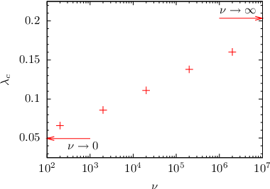
One can immediately see that in the $\nu\to\infty$ limit the solution of (25) is $r_{k}=1$. This implies $\tilde{\cal P}={\cal P}$ which results in the already noted limiting behavior with $\lambda_{c}=1/\langle k\rangle$. On the other hand, in the case of a static network, where $\nu=0$, $\rho_{k}$ is proportional to $k$ near the threshold, implying $r_{k}=k/\langle k\rangle$ and $\tilde{\mathcal{P}}=\mathcal{P}^{*}$, which results in $\lambda_{c}=\langle k\rangle/\langle k^{2}\rangle$.

Numerical solutions of (25) for intermediate values of $\nu$ are shown in Fig. 2. One can see that for a large but finite $\nu$ there are two crossover values of $k$. For $k$ below some value $k_{1}$ one has $r_{k}=1$ and $\tilde{\mathcal{P}}=\mathcal{P}$ (infinite rewiring), whereas for $k$ larger than some other value $k_{2}$, one has $r_{k}=k/\langle k\rangle$ and $\tilde{\mathcal{P}}=\mathcal{P}^{*}$ (static). Between $k_{1}$ and $k_{2}$ we find an intermediate regime, which connects the two extreme cases. The crossover values $k_{1}$ and $k_{2}$ increase with increasing $\nu$.

Using these numerical solutions for $r_{k}$ we calculated numerically the effect of rewiring on the threshold $\lambda_{c}$ by using (26). Results are shown in Fig. 2. One can clearly see that as the rewiring rate increases the threshold increases.

As discussed above, for SF networks with $2<\gamma\leq 3$ there is no threshold in the infection rate, and the prevalence is non-zero for any $\lambda>0$. For SF networks with $\gamma>3$ a threshold exists such that for an infection rate below $\lambda<\lambda_{c}$ the prevalence is zero. The prevalence corresponding to such networks is studied in this section using numerical simulations of finite networks.

The networks were constructed using two sets of parameter values for the rewiring dynamics (11). As an example of a network with $2<\gamma\leq 3$ we use the dynamics with $v(k)=1/N$, $u(k)=1+b/k$ ($k_{0}=1$) and $b=2.5$ . As described previously, $\langle k\rangle=1/(b-2)=2$ corresponds to the critical average value of the underlying zero-range process for which the steady state degree distribution is a power law with $\gamma=2.5$. The resulting prevalence as a function of the infection rate is plotted in Fig. 3(a) for various rewiring rates.

As an example of a network with $\gamma>3$ we used the dynamics (11) with $\langle k\rangle\approx 4.917$, $b=3.5$ and $k_{0}=15$, corresponding to the critical average value of the underlying zero-range process for which the steady state degree distribution is a power law with $\gamma=3.5$. The resulting prevalence as a function of the infection rate is plotted in Fig. 4(a) for various rewiring rates.

For a network of finite size, there is no true threshold but a crossover infection rate which is obtained for a quasi-stationary state. In simulations one can identify this crossover value $\lambda_{c}(N,L)$ as the point where the (numerically obtained) derivative $\mathrm{d}\rho/\mathrm{d}\lambda$ takes its maximum. With such a definition $\lambda_{c}(N,L)\to\lambda_{c}$ in the thermodynamic limit. One can see in Fig. 3(b), corresponding to $2<\gamma<3$, that as the rewiring rate increases $\lambda_{c}(N,L)$ increases from approximately $\langle k\rangle/\langle k^{2}\rangle\approx 0.04$ towards $1/\langle k\rangle=0.5$. Similarly, one can see in Fig. 4(b), corresponding to $\gamma>3$, that as the rewiring rate increases $\lambda_{c}(N,L)$ increases from approximately $\langle k\rangle/\langle k^{2}\rangle\approx 0.07$ towards $1/\langle k\rangle=0.2$.

In the simulations a very weak external source of infection was introduced in order to prevent the system from fluctuating into the absorbing state. There are several other methods of simulating an absorbing phase transition and computing from it the value of the threshold which are reviewed in [25].

Note that for the considered value of $b=2.5$, $\langle k^{2}\rangle$ diverges in the thermodynamic limit, therefore, based on the MF results, the threshold is expected to vanish for $\nu=0$. However, for a finite system one expects a finite crossover value for $\lambda$, which is of order $1/\langle k^{2}\rangle$. On the other hand, for $\nu\gg\langle k^{2}\rangle$ the crossover value should increase up to $1/\langle k\rangle$. It is interesting to examine how the crossover $\lambda$ changes if the rewiring rate is of order $\langle k^{2}\rangle$. To this end we performed simulations with $\nu\sim\langle k^{2}\rangle$. We found that the threshold scales as $\lambda_{c}^{-1}\sim\langle k^{2}\rangle$. The corresponding data collapse is presented in Fig. 5 where the prevalence is plotted as a function of a scaled infection rate $\lambda_{c}\langle k^{2}\rangle$ for networks of different sizes with a rewiring rate equal to the second moment of the degree distribution $\nu=\langle k^{2}\rangle$.

In Fig. 6 and Fig. 7 the simulation results are compared to the numerical solution of (14) for $b=2.5$ and $b=3.5$ for both a static network ($\nu=0$) and for $\nu=10^{4}$. The numerical calculation of the MF contact equation was carried out by solving (13) for each infection rate. The degree distribution used in the calculation was taken from the simulation results. For both the $b=2.5$ and $b=3.5$ cases the MF solution for $\nu=10^{4}$ agrees quite well with the simulation results which supports our general argument that as the rewiring rate increases, compared to the infection process, both the degree of a node and fluctuations average out such that the MF approximation better describes the process.

References

- [1] F. Liljeros, C. R. Edling, L. A. N. Amaral, H. E. Stanley, and Y. Aberg, Nature 411, 907 (2001).
- [2] A. L. Lloyd and R. M. May, Science 292, 1316 (2001).
- [3] M. E. J. Newman, S. Forrest, and J. Balthrop, Phys. Rev. E 66, 035101 (2002).
- [4] S. N. Dorogovtsev, A. V. Goltsev, and J. F. F. Mendes, Reviews of Modern Physics 80, 1275 (2008).
- [5] A. Barrat, M. Barthelemy, and A. Vespignani, Dynamical processes in complex networks (Cambridge University Press, 2008).
- [6] A.-L. Barabasi and R. Albert, Science 286, 509 (1999).
- [7] A.-L. Barabasi, R. Albert, and H. Jeong, Physica A: Statistical Mechanics and its Applications 272, 173 (1999).
- [8] A.-L. Barabasi, R. Albert, and H. Jeong, Physica A: Statistical Mechanics and its Applications 281, 69 (2000).
- [9] R. Albert and A. L. Barabasi, Reviews of Modern Physics 74, 47 (2002).
- [10] R. Pastor-Satorras and A. Vespignani, Phys. Rev. Lett. 86, 3200 (2001a).
- [11] R. Pastor-Satorras and A. Vespignani, Phys. Rev. E 63, 066117 (2001b).
- [12] R. Pastor-Satorras and A. Vespignani, Phys. Rev. E 65, 035108 (2002a).
- [13] M. Boguñá, R. Pastor-Satorras, and A. Vespignani, Lect. Notes Phys. 625, 127 (2003).
- [14] S. N. Dorogovtsev and J. F. F. Mendes, Evolution of networks (Oxford University Press, 2003).
- [15] M. R. Evans and T. Hanney, Math.Gen. 38, R195 (2005).
- [16] A. G. Angel, M. R. Evans, E. Levine, and D. Mukamel, Phys. Rev. E 72, 046132 (2005).
- [17] R. Pastor-Satorras and A. Vespignani, Phys. Rev. E 65, 036104 (2002b).
- [18] P. Erdős and A. Rënyi, Publ. Math. Inst. Hung. Acad. Sci 5, 17 (1960).
- [19] M. Boguñá, R. Pastor-Satorras, and A. Vespignani, The European Physical Journal B 38, 205 (2004).
- [20] T. Gross, C. J. D. D’Lima, and B. Blasius, Phys. Rev. Lett. 96, 208701 (2006).
- [21] E. Volz and L. A. Meyers, Proceedings of the Royal Society B: Biological Sciences 274, 2925 (2007).
- [22] N. H. Fefferman and K. L. Ng, Phys. Rev. E 76, 031919 (2007).
- [23] L. B. Shaw and I. B. Schwartz, Phys. Rev. E 77, 066101 (pages 10) (2008).
- [24] L. B. Shaw and I. B. Schwartz, in Adaptive Networks: Theory, Models and Applications, edited by T. Gross and H. Sayama (Springer/NECSI, 2009), Studies on Complexity Series.
- [25] M. M. de Oliveira and R. Dickman, Phys. Rev. E 71, 016129 (pages 5) (2005).