Jump-diffusion modeling in emission markets

Emission Trading Schemes (ETSs) have recently been designed with the main aim to reduce emissions of greenhouse gases and other pollutants. Two examples of ETSs are the EU ETS (European Union Emission Trading Scheme) and the US Sulfur Dioxide Trading System. In such schemes, the regulator allocates each market participant a number of credits, each of which gives the holder the right to emit a specified amount of pollutant (e.g. CO₂). At the end of a compliance period, each agent should not have released more pollutant than covered by the credits it holds at that time, or it will have to pay a fine proportional to the excess of the pollutant amount over the one corresponding to the credits held. During the compliance period, however, each agent can trade credits with other market participants, depending on whether it is cheaper to reduce emission or to buy credits.

The present study relies on a detailed mathematical model for such a scheme based on market equilibrium. We exploit its implications for the risk neutral allowance price evolution. The key issue is a feedback relationship between allowance prices and pollution abatement activity. Namely, any increase in allowance price enforces emission reduction since agents would then tend to sell their allowances. Hence the increase of the allowance price encourages supply of certificates and lowers the probability of non-compliance, which, in its turn, tends to diminish allowance prices. Following [15], we describe this feedback relationship in terms of market fundamentals, using a stylized evolution of the expected non-compliance and emission savings costs. We pay particular attention to discontinuities in the information flow, assuming that some events may cause market participants to change their views on the future reduction volumes required to reach compliance. We show how risk neutral allowance price reacts to such “information discontinuity” and study this effect in derivatives valuation.

The paper is organized as follows. In Section 2, we extend the discrete-time framework from [15] to the continuous-time setting. In Section 3, we interpret our results in the context of diffusion processes, derive the corresponding partial differential equations and discuss option pricing. Section 4 is devoted to modeling shock events in the information flow. Our description is based on jump-diffusion processes and requires solving a nonlinear partial integro-differential equation. We show that solutions to these non-linear equations from Section 3 and 4 satisfy the maximum principle. In the last section we propose a numerical implementation of its solution. In particular, we prove that the discretized problem possesses a unique solution and satisfies the maximum principle.

The suggested allowance price model is suitable for option pricing. It turns out that the fair price dynamics of European options written on emission allowance prices can be obtained by solving a linear partial integro-differential equation. We illustrate our results by numerical examples.

The literature on this subject is rather extensive, and we refer the interested reader to a nice expository work [27] which reviews the fundamental concepts of the environmental economics and provides a valuable guide to publications, which, however, is far from being complete. The economic theory of allowance trading goes back to [12] and [21], where the authors proposed trading the public good environment by means of transferable permits. Important results in dynamic allowance trading were obtained in [11], [28], [23], [19], [24], [26], [20] and in the literature cited therein. Recently, after the introduction of the real-world emission market EU ETS, the empirical evidence has become available. The experience gained from the operation of Phase I of the EU ETS is discussed in [13], and a detailed analysis of spot and futures allowance prices from this market is given in [29] and [30]. The contributions [2] and [22] are devoted to econometric modeling of emission allowance prices. Beyond confirming stylized facts of financial time series for prices of emission allowances, Markov switch and AR-GARCH models are suggested. The modeling of dynamic price equilibrium is addressed in [4] and [5], which provide a mathematical analysis of the market equilibrium and use optimal stochastic control theory to show social optimality of emission trading schemes. A recent work [15] considers equilibrium of risk averse market players and elaborates on risk neutral dynamics. The problems of derivatives valuation in emission markets are also addressed. The paper [8] discusses an endogenous emission permit price dynamics within equilibrium setting and elaborates on the valuation of European options on emission allowances. The dissertation [31] and the paper [25] deal with the risk-neutral allowance price formation within the EU ETS. In that paper, when utilizing equilibrium properties, the price evolution is treated in terms of marginal abatement costs and optimal stochastic control. The work [7] is also devoted to option pricing within EU ETS. The authors suppose that the drift of allowance spot prices is related to a hidden variable, which describes the overall market position in allowance contracts, and make use of filtering techniques to derive option price formulas which reflect specific allowance banking regulations valid in the EU ETS. Finally, the recent work [6] presents an approach where emission certificate futures are modeled in terms of a deterministic time change applied to a certain class of interval-valued diffusion processes.

During the compliance period (typically 3–5 years), each ETS participant dynamically adjusts its production processes (and hence its emissions) and trades emission credits at times $t=0,1,2,\ldots,T<\infty$ to maximize its revenue. In this setting, allowance price reaches its equilibrium determined by supply and demand of emission allowances. In what follows, we base on the model from [15] which characterizes the equilibrium allowance prices in terms of non-compliance uncertainty and abatement costs. This characterization forms the starting point for our analysis.

Let $\left(\Omega,{\cal F},\mathbf{P},\{{\cal F}_{t}\}_{t=0}^{T}\right)$ be a filtered probability space. We assume that all the processes considered in this section are adapted to $\{{\cal F}_{t}\}_{t=0}^{T}$. Consider a market with a finite set $I$ of agents who must comply with the ETS rules. Assume that, for each $i\in I$, an exogenously given stochastic process $\{E^{i}_{t}\}_{t=0}^{T-1}$ describes the so-called “business as usual” emission of agent $i$. That is, $E^{i}_{t}=E^{i}_{t}(\omega)$ stands for the total pollution of the agent $i$ which will be emitted during the time interval $(t,t+1]$ if no abatement measures are applied by the agent. Suppose that each agent $i$ can decide, at any time $t=0,\dots,T-1$, to perform a reduction of $\xi^{i}_{t}$ pollutant units to be emitted during $(t,t+1]$. The cost of abatement is modeled by a function of the reduced volume that can be random (reflecting the uncertainty in fuel prices). Thus, if at time $t=0,\dots,T-1$ agent $i$ decides on reduction by $x\in[0,\infty)$ units for the time interval $(t,t+1]$, then it costs it $C^{i}_{t}(x)=C^{i}_{t}(x)(\omega)$, where $C^{i}_{t}:[0,\infty)\times\Omega\mapsto[0,\infty)$ is ${\cal B}([0,\infty))\otimes{\cal F}_{t}$-measurable, and for each $\omega\in\Omega$, the mapping $x\mapsto C^{i}_{t}(x)(\omega)$ is strictly convex and continuous with $C_{t}(0)=0$. Therefore, following this abatement policy $\{\xi^{i}_{t}\}_{t=0}^{T-1}$, agent $i$ will have born by the compliance date $T$ the total abatement costs of

For each $i\in I$, $\omega\in\Omega$, $t=0,\dots,T-1$ and $a\in[0,\infty)$, we introduce the “reduction volume”

This quantity gives the “locally optimal” reduction volume for agent $i$ for the time period $(t,t+1]$ given that the price of one allowance unit is equal to $a$ for that time period; we may assume (and Proposition 2.1 (b) below supports this) that, being rational, agent $i$ will implement emission reduction at that level. As is well known (see e.g. [15]), under the above assumptions $r_{t}^{i}(a)(\omega)$ is a non-decreasing and continuous function of $a\in[0,\infty)$ for each $\omega\in\Omega$ and $t=0,\dots,T-1$. Next denote the total $t$-th time period reduction by

which represents the total reduction by all agents in the market for the time period $(t,t+1]$, given the time $t$ price of one allowance unit is $a$.

Suppose that, at any time $t=0,\dots,T$, credits can be traded at the spot price $A_{t}$. Denote by $\vartheta^{i}_{t}$ the change in the allowance number held by agent $i$ at time $t$. Then, given the allowance prices $\{A_{t}\}_{t=0}^{T}$, the position changes $\{\vartheta^{i}_{t}\}_{t=0}^{T}$ will result for agent $i$ in the total trading costs of

Here and in what follows, for simplicity’s sake we assume, zero interest rates (or, equivalently, that all the prices are already discounted).

Further, the total pollution of agent $i$ during the compliance interval $[0,T]$ can be expressed as the cumulative business-as-usual emission less the agent’s total reduction:

Denoting by $\gamma_{i}$ the agent’s initial allowance allocation, we observe that $i$ will hold $\gamma_{i}+\sum_{t=0}^{T}\vartheta^{i}_{t}$ allowances at time $T$ and hence its loss resulting from the potential penalty payment at rate $\pi$ (the penalty for the amount of emissions corresponding to one allowance) is

Finally, we define the space of feasible trading strategies $\vartheta^{i}=\{\vartheta^{i}_{t}\}_{t=0}^{T}$ and abatement strategies $\xi^{i}=\{\xi^{i}_{t}\}_{t=0}^{T-1}$ of agent $i\in I$ as

In view of (1), (4) and (5), the total revenue of agent $i$ following an admissible policy $(\vartheta^{i},\xi^{i})\in{\cal U}^{i}$ is equal to

To specify risk preferences, we describe agents’ risk attitudes by individual utility functions $U^{i}$, $i\in I$, that are assumed to be continuous strictly increasing and concave. For a random variable $X$, consider the utility functional

which is defined whenever the expectation exists and is not $-\infty$. Given an allowance price process $A=\{A_{t}\}_{t=0}^{T}$, agent $i$ behaves rationally in the sense that it maximizes its utility from the terminal wealth

by an appropriate choice of the strategy that we denote by $(\vartheta^{i*},\xi^{i*})$. Following the standard apprehension, a realistic market state is described by the so-called equilibrium — a situation where the allowance price, positions and abatement measures are such that each agent is satisfied with the own strategy and, at the same time, the natural restrictions are met.

In [15], this equilibrium notion was used to establish a reduced-form model which describes the allowance price evolution from the risk-neutral perspective. This approach utilizes the following three properties of the above equilibrium.

• (a)

  There is no arbitrage since any profitable strategy would immediately be followed by all agents.

• (b)

  Given a technology with lower reduction costs than the present allowance price, it is optimal to immediately reduce one’s pollution and take profit from selling allowances.

• (c)

  There are only two final outcomes for allowance price: at maturity, either the price will vanish if there is an excess in allowances, or, in the case of their shortage, the price will rise to the penalty level. Exact coincidences of allowance demand and supply at maturity occur with zero probability under broad assumptions and can be neglected.

The last property follows from the assumption that the random variable $\sum_{i}E_{T}^{i}$ representing the total emissions at maturity has a continuous distribution, given the information up to time $T-1$. Under mild additional assumptions, [15] claims that the above assertions can be deduced from the equilibrium in the following form.

In fact, Proposition 2.1 states the above-mentioned feedback relationship. Namely, the equilibrium allowance price process $\{A^{*}_{t}\}_{t=0}^{T}$ is a martingale under $\mathbf{Q}\sim\mathbf{P}$ that has the terminal value (7). However, this terminal random variable depends on the intermediate values $\{A^{*}_{t}\}_{t=0}^{T-1}$ through (6). A surprising consequence of the feedback relationship is that, from the risk-neutral perspective, only the cumulative market quantities are relevant. To see this, introduce the overall “business-as-usual” allowance shortage by

Further, recall from (3) the cumulative abatement function $r_{t}(a)$ to express the risk-neutral certificate price dynamics using (6) (7) and the martingale property of $\{A_{t}^{\ast}\}_{t=0}^{T}$ under $\mathbf{Q}$ as

Although the individual market attributes seem to be irrelevant here, the reader should notice that this picture appears only from the risk-neutral viewpoint.

With this, the problem of risk neutral allowance price modeling boils down to the following task:

In this form, transition to the continuous time case is straightforward and the resulting problem can be stated as follows:

Problem (8) is the starting point of our investigation in this paper. This approach utilizes the ingredients $\{r_{t}\}_{t\in[0,T]}$ and ${\cal E}_{T}$, which is reasonable from the practical perspective since the price-dependent reduction functions $\{r_{t}\}_{t\in[0,T]}$ can be estimated from the market data and the potential allowance shortage ${\cal E}_{T}$ can be modeled in terms of emission fluctuations.

Modeling in continuous time stipulates that the compliance period is an interval $[0,T]$ and that all the relevant random evolutions are described by adapted stochastic processes on a filtered probability space $(\Omega,{\cal F},\mathbf{Q},\{{\cal F}_{t}\}_{t\in[0,T]})$ which is equipped with a “spot martingale” probability measure $\mathbf{Q}\sim\mathbf{P}$. Given a random variable ${\cal E}_{T}$ and appropriate non-decreasing continuous abatement functions $r_{t}:\mathbb{R}_{+}\times\Omega\to\mathbb{R}_{+}$ indexed by $t\in[0,T]$, we want to find a solution $\{A_{t}\}_{t\in[0,T]}$ to

The results of the discrete-time analysis given in [15] suggest that, if the increments of the martingale

are independent and the abatement functions $r_{t}:\mathbb{R}_{+}\times\Omega\to\mathbb{R}_{+}$ are deterministic and time independent, then one can reasonably expect that a solution to (9) can have the functional form

with an appropriate deterministic function

and a state process $\{X_{t}\}_{t\in[0,T]}$ given by

In this section, we demonstrate how this approach enables one to find a solution in the framework of diffusion processes. Assume that $\{W_{t}\}_{t\in[0,T]}$ is a standard Brownian motion process (under $\mathbf{Q}\sim\mathbf{P}$) and that our $\{{\cal F}_{t}\}_{t\in[0,T]}$ is the natural filtration of the process. In this case, by the martingale representation theorem [16], one must have

for some admissible adapted process $\{\sigma_{t}\}_{t\in[0,T]}$. To ensure that $\{{\cal E}_{t}\}_{t\in[0,T]}$ has independent increments, we assume that $\{\sigma_{t}=\sigma(t)\}_{t\in[0,T]}$ is a known deterministic function and that we are given continuous non-decreasing time-independent abatement functions $\{r_{t}=r\}_{t\in[0,T]}$. To verify the martingale property of the allowance price process

we use Itô’s formula and (11) to write the stochastic differential of the process as

Here $[{\cal E}]_{t}$ stands for the quadratic variation of the martingale $\{{\cal E}_{t}\}_{t\in[0,T]}$ and $\partial_{(i,j)}$ denotes the respective partial derivatives. Now we observe that the function $\alpha$ is a solution to

in $(0,T)\times\mathbb{R}$ with the boundary condition

justified by the digital terminal allowance price, then the thus constructed $\{A_{t}\}_{t\in[0,T]}$ will indeed be a martingale that satisfies (9) by construction. Note that $\alpha(t,x)$ satisfies the maximum principle, so that $0\leqslant\alpha(t,x)\leqslant\pi$ for all $(t,x)\in[0,T]\times\mathbb{R}$. For the proof of this fact, see Proposition 4.1 below.

The following summarizes the above-presented approach.

Allowance price in the diffusion framework

1. 1.

   Given a continuous non-decreasing function $r:[0,\infty)\to[0,\infty)$ and a positive function $\sigma(t)$, $t\in[0,T]\times\mathbb{R}$, determine a solution $\alpha$ to the boundary value problem (12), (13). (We assume that $\sigma(t)$ is regular enough to ensure existence and uniqueness of the solution.)

2. 2.

   Verify that there is a unique strong solution to

   $$dX_{t}=d{\cal E}_{t}-r(\alpha(t,X_{t}))dt,\qquad X_{0}={\cal E}_{0}.$$

   (14)

3. 3.

   Introduce the allowance price $\{A_{t}\}_{t\in[0,T]}$ by

   $$A_{t}:=\alpha(t,X_{t}),\qquad t\in[0,T].$$

Having constructed the allowance price process $\{A_{t}\}_{t\in[0,T]}$ in this way, one obtains a standard procedure for the valuation of European options. Indeed, observe that, due to the Markov property of the strong solution to $(\ref{sde})$, the fair time $t$ price of a European call option written on the allowance price at (maturity) date $\tau\in(t,T]$ is given in terms of an appropriate function of the state variable:

To ensure that $\{C_{t}=f^{\tau}(t,X_{t})\}_{t\in[0,\tau]}$ is a martingale, the function $f^{\tau}:[0,\tau)\times\mathbb{R}\to\mathbb{R}$ is to be taken as a solution to the linear partial differential equation

in $(0,\tau)\times\mathbb{R}.$ However, the boundary condition in this case will be

Summarizing, we obtain the following description for the procedure.

Valuating a European call in the diffusion framework

1. 1.

   Find the function $\alpha$ as above.

2. 2.

   Given a strike price $K\geq 0$ and maturity time $\tau\in[0,T]$ of a European call, calculate $f^{\tau}$ as the solution to the boundary problem (15), (16).

3. 3.

   Given a time $t\in[0,\tau]$ and the allowance price $a\in[0,\pi]$ at time $t$, obtain $x$ as the solution to $\alpha(t,x)=a$.

4. 4.

   Substitute $t$ and the thus obtained $x$ into the function $f^{\tau}$ to obtain the time $t$ price of the European call as $f^{\tau}(t,x)$.

Note that one can also estimate $f^{\tau}$ directly using Monte Carlo simulations: given a strike price $K\geq 0$, a maturity time $\tau\in[0,T]$ of a European call, a time $t\in[0,\tau]$ and the allowance price $a\in[0,\pi]$ at time $t$, obtain $X_{t}=x$ as the solution to $\alpha(t,x)=a$. Then, using the Markov property of $\{X_{t}\}$, one can evaluate the option price

by estimating the expectation via simulating a (large enough) number $N_{MC}$ of copies of the random variable $X_{\tau}$.

Note that closed-form solutions to the non-linear partial differential equation (12) are rarely available. However, a linear abatement function leads to explicit expressions, as pointed out in [25] and [31]. We will consider this case as an illustration.
Example. Given a linear abatement function $r(a)=ca$, $c\in(0,\infty)$, and a constant diffusion coefficient $\{\sigma_{t}=\sigma\}_{t\in[0,T]}$ with $\sigma\in(0,\infty)$, the partial differential equation (12) becomes Burger’s equation

whose solution can be obtained from that of the heat equation via the Hopf-Cole transform.

Namely, a direct calculation shows that if $v:[0,T]\times\mathbb{R}\mapsto\mathbb{R}$ solves the heat equation

then its Hopf-Cole transform

solves (17). In order to satisfy an original boundary condition

the boundary value function for (18) must be chosen as

Our digital boundary condition has the form

so that we should take

Denoting by $\mathbf{N}(\mu,s^{2})$ the normal distribution with mean $\mu$ and variance $s^{2}$ and by $\Phi(y)$ and $\varphi(y)=\Phi^{\prime}(y)$ the standard normal distribution function and its density, respectively, we can write:

The derivative of this expression with respect to $x$ is equal to

Next we use (19) to calculate

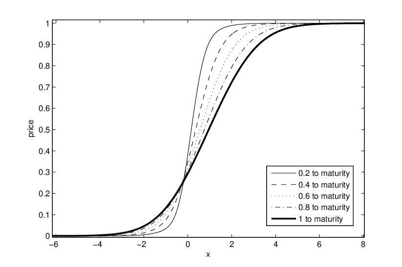
The shape of this function is depicted in Figure 1.

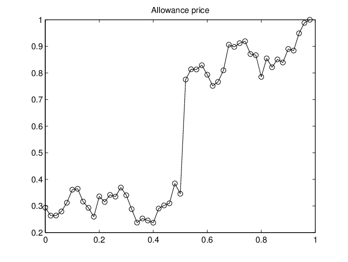
To illustrate our valuation procedure, consider the following parameters: time to compliance date $T=2$, diffusion coefficient $\sigma=4$, penalty $\pi=100$ and a linear abatement function $r(a)=ca$ with $c=0.02$. Taking $t=0$, we consider a family of European calls with the same strike price $K=25$, but different maturity times $\tau$. Suppose that the initial allowance price is equal to the strike price $a=A_{0}=25$ (the so-called at-the-money situation), which is attained by $\alpha(0,x)=25$ with $x\approx-2.434$. Next, we determine the call prices $C(0,\tau)$ at time $t=0$ for different maturity times $\tau\in[0,T]$. Independently of the model, the price of an expiring call with $\tau=0$ must be equal to zero, whereas the longest-maturity call with $\tau=T$ must have the price $A_{0}(\pi-K)/\pi=25\times 0.75=18.75$. (Note that, because of the digital payoff, such a call is equivalent to $0.75$ allowances). That is, the call prices increase with contract’s maturity from $0$ to $18.75$. The shape of this curve is obtained using a crude Monte Carlo procedure. We have simulated $N_{MC}=10^{4}$ i.i.d. copies of the random variable $X_{\tau}$. We used the forward Euler method to generate i.i.d. copies of $\{X_{t}\}$, with time step $0.02$. The curve is presented in Figure 2, together with $95\%$ confidence intervals.

In this section, we describe a situation where the market can suddenly change due to the presence of jumps. We propose a framework suitable to the present practice of the EU ETS where the member states negotiate their allowance allocations and the market needs to adapt to the new situation. For instance, revised decision on the amount of allocated certificates yields a jump of allowance market prices. Also, a sudden change in demand and/or price for fuel can result in the pollution levels changing dramatically which impacts on the allowance prices.

We discuss how to solve problem (8) in the jump-diffusion setting using a similar approach to the one employed in Section 3. Namely, we choose a candidate for (9) of the form

where $\alpha$ and $X_{t}$ are as in (10) and (11), respectively. But now we assume that the martingale

is modeled using a general jump-diffusion process adapted to a filtration $\{{\cal F}_{t}\}_{t\in[0,T]}$. In this setting, the process $\{X_{t}\}_{t\in[0,T]}$ is given by the following stochastic differential equation:

where $\mathbb{R}_{0}=\mathbb{R}\setminus\{0\}$, $\{W_{t}\}_{t\in[0,T]}$ is a Brownian motion adapted to the filtration $\{{\cal F}_{t}\}_{t\in[0,T]}$, and $p_{\nu}$ is an independent of $\{W_{t}\}_{t\in[0,T]}$ $\{{\cal F}_{t}\}_{t\in[0,T]}$-adapted random Poisson measure with intensity $q_{\nu}(dy\times dt)=\lambda\nu(dy)dt$, $\nu$ being a probability distribution on $\mathbb{R}$ and $\lambda\in(0,\infty)$ a positive constant. Expression (23) allows us to model jumps with great flexibility, as the distribution of the jump is state and time dependent. It is known that, under suitable Lipschitz and growth conditions on $r$, $\sigma$ and $a$, stochastic differential equation (23) possesses a unique strong solution [14].

We again use Itô’s lemma for $A_{t}=\alpha(t,X_{t})$ to find conditions on $\alpha$ under which the process $\{A_{t}\}_{t\in[0,T]}$ will be a martingale under $\mathbf{Q}$. Let $\tau=T-t$. For convenience, we introduce a new function $\beta(\tau,x)=\alpha(T-\tau,x)$ and, instead of (12), obtain the following nonlinear partial integro-differential equation for $\beta$:

$(\tau,x)\in[0,T]\times\mathbb{R}$, with the boundary condition

Under certain assumptions, jump-diffusion models for option pricing lead to partial integro-differential equations, see e.g. [1, 9]. Equation (24) differs from them in that it has a nonlinear coefficient $r(\beta(\tau,x))$. We assume that there exists a classical solution $\beta\in C^{1,2}([0,T)\times\mathbb{R})$ to the problem (24), (25). It is not difficult to see that it satisfies the maximum principle.

Note that Proposition 4.1 also proves the maximum principle for solution to the boundary value problem (12), (13).

We will see that, under a mild condition, the maximum principle remains valid for the discretized problem as well (see Proposition 4.2 below).

Analytical solution to partial integro-differential equations can only be obtained in a few special cases, so in most situations one can only solve them numerically. In this section, we discuss a discretization of (24) using the finite difference method and prove that the discretized equation has a unique solution. Finally, we illustrate the approach by providing a numerical example.

First we need to truncate the domain of $x$. Let $D_{l}:=\{x\in\mathbb{R}:\,|x|<l\}$, where the bound $l>0$ of the domain can be chosen so that the probability that the process $\{X_{t}\}$ leaves $D_{l}$ during the time interval $[0,T]$ given it starts at $X_{0}$ does not exceed a given small $\epsilon>0$. This procedure will be illustrated at the end of the section.

Next, we restrict the domain of integration for the integral term on the RHS of (24) to an interval $[K_{1},K_{2}]$, chosen such that the error made due to the truncation also remains small. For a good choice of the terminals $K_{j}$, one can refer to the study presented in [3].

The numerical solution will be computed on a discrete grid. Let $N$ denote the total number of discrete $x$-values and $M$ the total number of $\tau$-values we want to use in the grid for the numerical solution, so that the step sizes in $x$ and $\tau$ are respectively $\Delta_{x}=2l/N$ and $\Delta_{\tau}=T/M$. Put $x_{i}=-l+i\Delta_{x}$, $\tau_{n}=n\Delta_{\tau}$, for $i\in\mathbb{Z}$ and $n=0,\ldots,M$. We use $\beta_{i}^{n}=\beta(\tau_{n},x_{i})$ for the values of $\beta$ on this grid. Because of the presence of the non local term on the RHS of equation (24), one needs to define $\beta$ outside $[0,T]\times D_{l}$. We chose the simplest and most intuitive approach and set $\beta_{i}^{n}:=g(x_{i})$ for $i\notin\{0,\ldots,N-1\}$, where

The partial derivatives are replaced by the respective finite differences:

Following an approach similar to the one used in [10], we consider the same step size $\Delta_{x}$ to approximate the integral term, and choose $J_{1}$ and $J_{2}$ such that $[K_{1},K_{2}]\subseteq[(J_{1}-1/2)\Delta_{x},(J_{2}+1/2)\Delta_{x}]$, which leads to the approximation

where

and

References

- [1] Andersen, A. and Andreasen, J. (2000). Jump diffusion processes: Volatility smile fitting and numerical methods for option pricing, Rev. Derivatives Res. 4(3) 231–262.
- [2] E. Benz and S. Trueck (2008). Modeling the price dynamics of CO2 emission allowances, Bonn Graduate School of Economics
- [3] Briani, M., La Chioma, C. and Natalini, R. (2004). Convergence of numerical schemes for viscosity solutions to integro-differential degenerate parabolic problems arising in finance theory, Numerische Mathematik 98(4) 607–646.
- [4] R. Carmona and F. Fehr and J. Hinz (2009). Optimal stochastic control and carbon price formation, SIAM Journal on Control and Optimization
- [5] R. Carmona and F. Fehr and J. Hinz and A. Porchet (2009). Market Designs for Emissions Trading Schemes, preprint
- [6] R. Carmona and J. Hinz (2009). Risk Neutral Modeling of Emission Allowance Prices and Option Valuation, Technical Report, Princeton University
- [7] U. Cetin and M. Verschuere (2008). Pricing and hedging in carbon emissions markets, Technical Report, London School of Economics
- [8] M Chesney and L. Taschini (2009). The endogenous price dynamics of the emission allowances: An application to CO2 option pricing, Swiss Finance Institute Research Paper No. 08-02; EFA 2008 Athens Meetings Paper
- [9] Cont, R. and Tankov, P. (2004). Financial Modelling with Jump Processes, Chapman Hall
- [10] Cont, R. and Voltchkova, E. (2005). A finite diference scheme for option pricing in jump diffusion and exponential Lévy models, SIAM J. Numer. Anal. 43(4) 1596–1626.
- [11] Cronshaw, M. and Kruse, J. B. (1996). Regulated Firms in Pollution Permit Markets with Banking, Journal of Regulatory Economics 9(2) 179–89.
- [12] Dales, J. H. (1968). Pollution, Property and Prices University of Toronto Press, Toronto
- [13] G. Daskalakis and D. Psychoyios and R. N. Markellos (2009). Modeling CO2 Emission Allowance Prices and Derivatives: evidence from the European Trading Scheme, Journal of Banking Finance 33(7) 1230–1241.
- [14] Gikhman, I. I. and Skorokhod, A. V. (1972). Stochastic Differential Equations, Springer-Verlag
- [15] Hinz, J. and Novikov, A. (to appear). On fair pricing of emission-related derivatives, Bernoulli
- [16] I. Karatzas and S. Shreve (1991). Brownian Motion and Stochastic Differential Equations, Springer Verlag
- [17] Kloeden, P. E. and Platen, E. (1992). Numerical Solution of Stochastic Differential Equations, Berlin; New York : Springer-Verlag
- [18] Lancaster, P. (1969). Theory of Matrices, New York, Academic Press
- [19] Leiby, P. and Rubin, J. (2001). Intertemporal Permit Trading for the Control of Greenhouse Gas Emissions, Environmental and Resource Economics 19(3) 229–256.
- [20] Maeda, A. (2004). Impact of Banking and Forward Contracts on Tradable Permit Markets, Environmental Economics and Policy Studies 6(2) 81–102.
- [21] Montgomery, W. D. (1972). Markets in Licenses and Efficient Pollution Control Programs, Journal of Economic Theory 5(3) 395–418.
- [22] M. S. Paolella and L. Taschini (2008). An Econometric Analysis of Emissions Trading Allowances, Journal of Banking and Finance
- [23] Rubin, J. (1996). A Model of Intertemporal Emission Trading, Banking and Borrowing, Journal of Environmental Economics and Managemen 31(3) 269–286.
- [24] Schennach, S. M. (2000). The Economics of Pollution Permit Banking in the Context of Title IV of the 1990 Clean Air Act Amendments, Journal of Environmental Economics and Management 40(3) 189–21.
- [25] Seifert, J. and Uhrig-Homburg, M. and Wagner, M. (2008). Dynamic Behavior of carbon Spot Prices. Theory and Empirical Evidence, Journal of Environmental Economics and Management 56(2) 180–194.
- [26] B. Stevens and A. Rose (2002). A Dynamic Analysis of the Marketable Permits Approach to Global Warming Policy: a Comparison of Spatial and Temporal Flexibility, Journal of Environmental Economics and Management 44 45–69.
- [27] Taschini, L. (to appear). Environmental Economics and Modeling Marketable Permits: A Survey, Asian Pacific Financial Markets
- [28] Tietenberg, T. (1985). Emissions Trading: An Exercise in Reforming Pollution Policy, Resources for the Future, Boston
- [29] M. Uhrig-Homburg and M. Wagner (2007). Derivatives Instruments in the EU Emissions Trading Scheme, and Early Market Perspective, Technical Report, University of Karlsruhe
- [30] M. Uhrig-Homburg and M. Wagner (2007). Futures Price Dynamics of CO2 Emissions Certificates: an Empirical Analysis, Technical Report, University of Karlsruhe
- [31] M. Wagner (2006). Emissionszertifikate, Preismodellierung und Derivatebewertung PhD thesis, Universität Karlsruhe