Secure Communication in
Stochastic Wireless NetworksThanks: The present document is a draft submitted for publication on November 24, 2009.Thanks: P. C. Pinto and M. Z. Win are with the Laboratory for Information and Decision Systems (LIDS), Massachusetts Institute of Technology, Room 32-D674, 77 Massachusetts Avenue, Cambridge, MA 02139, USA (e-mail: ppinto@mit.edu, moewin@mit.edu). J. Barros is with Departamento de Engenharia Electrotécnica e de Computadores, Faculdade de Engenharia da Universidade do Porto, Portugal (e-mail: jbarros@fe.up.pt).Thanks: This research was supported, in part, by the Portuguese Science and Technology Foundation under grant SFRH-BD-17388-2004; the MIT Institute for Soldier Nanotechnologies; the Office of Naval Research under Presidential Early Career Award for Scientists and Engineers (PECASE) N00014-09-1-0435; and the National Science Foundation under grant ECS-0636519.

Pedro C. Pinto Student Member, IEEE João Barros Member, IEEE Affiliation: and Moe Z. Win, Fellow, IEEE Affiliation: Affiliation: Affiliation: Affiliation: Corresponding Address: Affiliation: Pedro C. Pinto Affiliation: Laboratory for Information and Decision Systems (LIDS) Affiliation: Massachusetts Institute of Technology (MIT) Affiliation: 77 Massachusetts Avenue, Room 32-D674 Affiliation: Cambridge, MA 02139 USA Affiliation: Affiliation: Tel.: (857) 928-6444 Affiliation: e-mail: ppinto@mit.edu

Abstract

Information-theoretic security – widely accepted as the strictest notion of security – relies on channel coding techniques that exploit the inherent randomness of the propagation channels to significantly strengthen the security of digital communications systems. Motivated by recent developments in the field, this paper aims at a characterization of the fundamental secrecy limits of wireless networks. Based on a general model in which legitimate nodes and potential eavesdroppers are randomly scattered in space, the intrinsically secure communications graph ( $i\mathcal{S}\textrm{-}$ graph) is defined from the point of view of information-theoretic security. Conclusive results are provided for the local connectivity of the Poisson $i\mathcal{S}\textrm{-}$ graph, in terms of node degrees and isolation probabilities. It is shown how the secure connectivity of the network varies with the wireless propagation effects, the secrecy rate threshold of each link, and the noise powers of legitimate nodes and eavesdroppers. Sectorized transmission and eavesdropper neutralization are explored as viable strategies for improving the secure connectivity. Lastly, the maximum secrecy rate between a node and each of its neighbours is characterized, and the case of colluding eavesdroppers is studied. The results help clarify how the spatial density of eavesdroppers can compromise the intrinsic security of wireless networks.

Index Terms:

Physical-layer security, wireless networks, stochastic geometry, secure connectivity, node degree, secrecy capacity, colluding eavesdroppers.

I Introduction

Contemporary security systems for wireless networks are based on cryptographic primitives that generally ignore two key factors: (a) the physical properties of the wireless medium, and (b) the spatial configuration of both the legitimate and malicious nodes. These two factors are important since they affect the communication channels between the nodes, which in turn determine the fundamental secrecy limits of a wireless network. In fact, the inherent randomness of the physics of the wireless medium and the spatial location of the nodes can be leveraged to provide intrinsic security of the communications infrastructure at the physical-layer level.¹¹ 1 In the literature, the term “security” typically encompasses 3 different characteristics: secrecy (or privacy), integrity, and authenticity. This paper does not consider the issues of integrity or authenticity, and the terms “secrecy and “security” are used interchangeably.

The basis for information-theoretic security, which builds on the notion of perfect secrecy [1], was laid in [2] and later in [3]. Moreover, almost at the same time, the basic principles of public-key cryptography, which lead to the predominance of computational security, were published in [4]. More recently, there has been a renewed interest in information-theoretic security over wireless channels. Space-time signal processing techniques for secure communication over wireless links are introduced in [5]. The secrecy of cooperative relay broadcast channels is considered in [6]. The case of a fixed number of colluding eavesdroppers placed at the same location is analyzed in [7]. The scenario of compound wiretap channels is considered in [8]. The capacity of cognitive interference channels with secrecy constraints is analyzed in [9]. The achievable secret communication rates using multiple-input multiple-output communications are investigated in [10, 11, 12, 13, 14]. The secrecy capacity of various degraded fading channels is established in [15]. A detailed characterization of the outage secrecy capacity of slow fading channels is provided in [16]. The ergodic secrecy capacity of fading channels was derived independently in [17, 18, 19]. The notion of strong secrecy for wireless channels is introduced in [20]. Some secrecy properties of random geometric graphs were presented in [21].

We are interested in the fundamental secrecy limits of large-scale wireless networks. The spatial location of the nodes can be modeled either deterministically or stochastically. Deterministic models include square, triangular, and hexagonal lattices in the two-dimensional plane [22, 23, 24], which are applicable when the position of the nodes in the network is known exactly or is constrained to a regular structure. In contrast, in many important scenarios, only a statistical description of the node positions is available, and thus a stochastic spatial model is the natural choice. In particular, the Poisson point process [25] has been successfully used in the context of wireless networks, most notably in what concerns connectivity and coverage [26, 27, 28], throughput [29, 30], interference [31, 32, 33, 34], environmental monitoring [35], and sensor cooperation [36], among other topics.

In this paper, we aim at a mathematical characterization of the secrecy properties of stochastic wireless networks. The main contributions are as follows:

•

Framework for intrinsic security in stochastic networks: We introduce an information-theoretic definition of the intrinsically secure communications graph ( $i\mathcal{S}\textrm{-}$ graph), based on the notion of strong secrecy. Our framework considers spatially scattered users and eavesdroppers, subject to generic wireless propagation characteristics.
•

Local connectivity in the $i\mathcal{S}\textrm{-}$ graph: We provide a complete probabilistic characterization of both in-degree and out-degree of a typical node in the Poisson $i\mathcal{S}\textrm{-}$ graph, using fundamental tools of stochastic geometry.
•

Techniques for communication with enhanced secrecy: We proposed sectorized transmission and eavesdropper neutralization as two techniques for enhancing the secrecy of communication, and quantify their effectiveness in terms of the resulting average node degrees.
•

Maximum secrecy rate (MSR) in the $i\mathcal{S}\textrm{-}$ graph: We provide a complete probabilistic characterization of the MSR between a typical node of the Poisson $i\mathcal{S}\textrm{-}$ graph and each of its neighbors. In addition, we derive expressions for the probability of existence of a non-zero MSR, and the probability of secrecy outage.
•

The case of colluding eavesdroppers: We provide a characterization of the MSR and average node degrees for scenarios in which the eavesdroppers are allowed to collude, i.e, exchange and combine information. We quantify exactly how eavesdropper collusion degrades the secrecy properties of the legitimate nodes, in comparison to a non-colluding scenario.

This paper is organized as follows. Section II describes the system model. Section III characterizes local connectivity in the Poisson $i\mathcal{S}\textrm{-}$ graph. Section IV analyzes two techniques for enhancing the secrecy of communication. Section V considers the MSR between a node and its neighbours. Section VI characterizes the case of colluding eavesdroppers. Section VII concludes the paper and summarizes important findings.

II System Model

We start by describing our system model and defining our measures of secrecy. The notation and symbols used throughout the paper are summarized in Table I.

II-A Wireless Propagation Characteristics

In a wireless environment, the received power $P_{\mathrm{rx}}(x_{i},x_{j})$ associated with the link $\overrightarrow{x_{i}x_{j}}$ can be written as

P_{\mathrm{rx}}(x_{i},x_{j})=P_{\ell}\cdot g(x_{i},x_{j},Z_{x_{i},x_{j}}),

(1)

where $P_{\ell}$ is the (common) transmit power of the legitimate nodes; and $g(x_{i},x_{j},Z_{x_{i},x_{j}})$ is the power gain of the link $\overrightarrow{x_{i}x_{j}}$ , where the random variable (RV) $Z_{x_{i},x_{j}}$ represents the random propagation effects (such as multipath fading or shadowing) associated with link $\overrightarrow{x_{i}x_{j}}$ . We consider that the $Z_{x_{i},x_{j}},x_{i}\neq x_{j}$ are independent identically distributed (IID) RVs with common probability density function (PDF) $f_{Z}(z)$ , and that $Z_{x_{i},x_{j}}=Z_{x_{j},x_{i}}$ due to channel reciprocity. The channel gain $g(x_{i},x_{j},Z_{x_{i},x_{j}})$ is considered constant (quasi-static) throughout the use of the communications channel, which corresponds to channels with a large coherence time. The gain function is assumed to satisfy the following conditions:

1.

$g(x_{i},x_{j},Z_{x_{i},x_{j}})$ depends on $x_{i}$ and $x_{j}$ only through the link length $|x_{i}-x_{j}|$ ; with abuse of notation, we can write $g(r,z)\triangleq g(x_{i},x_{j},z)|_{|x_{i}-x_{j}|\rightarrow r}$ .
2.

$g(r,z)$ is continuous and strictly decreasing in $r$ .
3.

$\lim_{r\rightarrow\infty}g(r,z)=0$ .

The proposed model is general enough to account for common choices of $g$ . One example is the unbounded model where $g(r,z)=\frac{z}{r^{2b}}$ . The term $\frac{1}{r^{2b}}$ accounts for the far-field path loss with distance, where the amplitude loss exponent $b$ is environment-dependent and can approximately range from $0.8$ (e.g., hallways inside buildings) to $4$ (e.g., dense urban environments), with $b=1$ corresponding to free space propagation. This model is analytically convenient [31], but since the gain becomes unbounded as the distance approaches zero, it must be used with care for extremely dense networks. Another example is the bounded model where $g(r,z)=\frac{z}{1+r^{2b}}$ . This model has the same far-field dependence as the unbounded model, but eliminates the singularity at the origin. Unfortunately, it often leads to intractable analytical results. The effect of the singularity at $r=0$ on the performance evaluation of a wireless system is considered in [37].

Furthermore, by appropriately choosing of the distribution of $Z_{x_{i},x_{j}}$ , both models can account for various random propagation effects [31], including:

1.

Path loss only: $Z_{x_{i},x_{j}}=1$ .
2.

Path loss and Nakagami- $m$ fading: $Z_{x_{i},x_{j}}=\alpha_{x_{i},x_{j}}^{2}$ , where $\alpha_{x_{i},x_{j}}^{2}\sim\mathcal{G}(m,\frac{1}{m})$ .²² 2 We use $\mathcal{G}(x,\theta)$ to denote a gamma distribution with mean $x\theta$ and variance $x\theta^{2}$ .
3.

Path loss and log-normal shadowing: $Z_{x_{i},x_{j}}=\exp(2\sigma_{\mathrm{s}}G_{x_{i},x_{j}})$ , where $G_{x_{i},x_{j}}\sim\mathcal{N}(0,1)$ .³³ 3 We use $\mathcal{N}(\mu,\sigma^{2})$ to denote a Gaussian distribution with mean $\mu$ and variance $\sigma^{2}$ . The term $\exp(2\sigma_{\mathrm{s}}G_{x_{i},x_{j}})$ has a log-normal distribution, where $\sigma_{\mathrm{s}}$ is the shadowing coefficient.
4.

Path loss, Nakagami- $m$ fading, and log-normal shadowing: $Z_{x_{i},x_{j}}=\alpha_{x_{i},x_{j}}^{2}\exp(2\sigma_{\mathrm{s}}G_{x_{i},x_{j}})$ , where $\alpha_{x_{i},x_{j}}^{2}\sim\mathcal{G}(m,\frac{1}{m})$ , $G_{x_{i},x_{j}}\sim\mathcal{N}(0,1)$ , with $\alpha_{x_{i},x_{j}}$ independent of $G_{x_{i},x_{j}}$ .

II-B Wireless Information-Theoretic Security

We now define our measure of secrecy more precisely. While our main interest is targeted towards the behavior of large-scale networks, we briefly review the setup for a single legitimate link with a single eavesdropper. The results thereof will serve as basis for the notion of $i\mathcal{S}\textrm{-}$ graph to be established later.

Consider the model depicted in Fig. 1, where a legitimate user (Alice) wants to send messages to another user (Bob). Alice encodes a message $s$ , represented by a discrete RV, into a codeword, represented by the complex random sequence of length $n$ , $x^{n}=(x(1),\ldots,x(n))\in\mathbb{C}^{n}$ , for transmission over the channel. Bob observes the output of a discrete-time channel (the legitimate channel), which at time $i$ is given by

y_{\ell}(i)=h_{\ell}\cdot x(i)+w_{\ell}(i),\quad 1\leq i\leq n,

where $h_{\ell}\in\mathbb{C}$ is the quasi-static amplitude gain of the legitimate channel,⁴⁴ 4 The amplitude gain $h_{\L}$ can be related to the power gain in (1) as $g(r_{\ell},Z_{\ell})=|h_{\ell}|^{2}$ , where $r_{\ell}$ and $Z_{\ell}$ are, respectively, the length and random propagation effects of the legitimate link. and $w_{\ell}(i)\sim\mathcal{N}_{\mathrm{c}}(0,\sigma_{\ell}^{2})$ is AWGN with power $\sigma_{\ell}^{2}$ per complex sample.⁵⁵ 5 We use $\mathcal{N}_{\textrm{c}}(0,\sigma^{2})$ to denote a CS complex Gaussian distribution, where the real and imaginary parts are IID $\mathcal{N}(0,\sigma^{2}/2)$ . Bob makes a decision $\hat{s}_{\ell}$ on $s$ based on the output $y_{\ell}$ , incurring in an error probability equal to $\mathbb{P}\{\hat{s}_{\ell}\neq s\}.$ A third party (Eve) is also capable of eavesdropping on Alice’s transmissions. Eve observes the output of a discrete-time channel (the eavesdropper’s channel), which at time $i$ is given by

y_{\mathrm{e}}(i)=h_{\mathrm{e}}\cdot x(i)+w_{\mathrm{e}}(i),\quad 1\leq i\leq n,

where $h_{\mathrm{e}}\in\mathbb{C}$ is the quasi-static amplitude gain of the eavesdropper channel, and $w_{\mathrm{e}}(i)\sim\mathcal{N}_{\mathrm{c}}(0,\sigma_{\textrm{e}}^{2})$ is AWGN with power $\sigma_{\textrm{e}}^{2}$ per complex sample. It is assumed that the signals $x$ , $h_{\ell}$ , $h_{\mathrm{e}}$ , $w_{\ell}$ , and $w_{\mathrm{e}}$ are mutually independent. Each codeword transmitted by Alice is subject to the average power constraint of $P_{\ell}$ per complex symbol, i.e.,

\frac{1}{n}\sum_{i=1}^{n}\mathbb{E}\{|x(i)|^{2}\}\leq P_{\ell}.

(2)

We define the transmission rate between Alice and Bob as

\mathpzc{R}\triangleq\frac{H(s)}{n},

where $H(\cdot)$ denotes the entropy function.

Throughout the paper, we use strong secrecy as the condition for information-theoretic security, and define it as follows [38].

Definition II.1 (Strong Secrecy)

The rate $\mathpzc{R}^{\!\!*}$ is said to be achievable with strong secrecy if $\forall\epsilon>0$ , for sufficiently large $n$ , there exists an encoder-decoder pair with rate $\mathpzc{R}$ satisfying the following conditions:

	$\displaystyle\mathpzc{R}$	$\displaystyle\geq\mathpzc{R}^{\!\!*}-\epsilon,$
	$\displaystyle H(s\|y_{\mathrm{e}}^{n})$	$\displaystyle\geq H(s)-\epsilon,$
	$\displaystyle\mathbb{P}\{\hat{s}_{\ell}\neq s\}$	$\displaystyle\leq\epsilon.$

We define the maximum secrecy rate (MSR) $\mathpzc{R}_{\mathrm{s}}$ of the legitimate channel to be the maximum rate $\mathpzc{R}^{\!\!*}$ that is achievable with strong secrecy.⁶⁶ 6 See [20] for a comparison between the concepts of weak and strong secrecy. In the case of Gaussian noise, the MSR is the same under the weak and strong secrecy conditions. If the legitimate link operates at a rate below the MSR $\mathpzc{R}_{\mathrm{s}}$ , there exists an encoder-decoder pair such that the eavesdropper is unable to obtain additional information about $s$ from the observation $y_{\mathrm{e}}^{n}$ , in the sense that $H(s|y_{\mathrm{e}}^{n})$ approaches $H(s)$ as the codeword length $n$ grows. It was shown in [39, 16] that for a given realization of the channel gains $h_{\ell},h_{\mathrm{e}}$ , the MSR of the Gaussian wiretap channel is

\mathpzc{R}_{\mathrm{s}}(x_{i},x_{j})=\left[\log_{2}\left(1+\frac{P_{\ell}\cdot|h_{\ell}|^{2}}{\sigma_{\ell}^{2}}\right)-\log_{2}\left(1+\frac{P_{\ell}\cdot|h_{\mathrm{e}}|^{2}}{\sigma_{\textrm{e}}^{2}}\right)\right]^{+},

(3)

in bits per complex dimension, where $[x]^{+}=\max\{x,0\}$ .⁷⁷ 7 Operationally, the MSR $\mathpzc{R}_{\mathrm{s}}$ can be achieved if Alice first estimates $h_{\ell}$ and $h_{\mathrm{e}}$ (i.e., has full CSI), and then uses a code that achieves MSR in the AWGN channel. Estimation of $h_{\mathrm{e}}$ is possible, for instance, when Eve is another active user in the wireless network, so that Alice can estimate the eavesdropper’s channel during Eve’s transmissions. As we shall see, the $i\mathcal{S}\textrm{-}$ graph model presented in this paper relies on an outage formulation, and therefore does not make assumptions concerning availability of full CSI. In the next sections, we use these basic results to analyze secrecy in large-scale networks.

II-C $i\mathcal{S}\textrm{-}$ Graph

Consider a wireless network where legitimate nodes and potential eavesdroppers are randomly scattered in space, according to some point process. The $i\mathcal{S}\textrm{-}$ graph is a convenient geometrical representation of the information-theoretically secure links that can be established on such network. In the following, we introduce a precise definition of the $i\mathcal{S}\textrm{-}$ graph, based on the notion of strong secrecy.

Definition II.2 ( $i\mathcal{S}\textrm{-}$ graph)

Let $\Pi_{\ell}=\{x_{i}\}\subset\mathbb{R}^{d}$ denote the set of legitimate nodes, and $\Pi_{\textrm{e}}=\{e_{i}\}\subset\mathbb{R}^{d}$ denote the set of eavesdroppers. The $i\mathcal{S}\textrm{-}$ graph is the directed graph $G=\{\Pi_{\ell},\mathcal{E}\}$ with vertex set $\Pi_{\ell}$ and edge set

\mathcal{E}=\{\overrightarrow{x_{i}x_{j}}:\mathpzc{R}_{\mathrm{s}}(x_{i},x_{j})>\varrho\},

(4)

where $\varrho$ is a threshold representing the prescribed infimum secrecy rate for each communication link; and $\mathpzc{R}_{\mathrm{s}}(x_{i},x_{j})$ is the MSR, for a given realization of the channel gains, of the link between the transmitter $x_{i}$ and the receiver $x_{j}$ , given by

\mathpzc{R}_{\mathrm{s}}(x_{i},x_{j})=\left[\log_{2}\left(1+\frac{P_{\mathrm{rx}}(x_{i},x_{j})}{\sigma_{\ell}^{2}}\right)-\log_{2}\left(1+\frac{P_{\mathrm{rx}}(x_{i},e^{*})}{\sigma_{\textrm{e}}^{2}}\right)\right]^{+},

(5)

with

e^{*}=\underset{e_{k}\in\Pi_{\textrm{e}}}{\mathrm{argmax}}\>P_{\mathrm{rx}}(x_{i},e_{k}).

(6)

This definition presupposes that the eavesdroppers are not allowed to collude (i.e., they cannot exchange or combine information), and therefore only the eavesdropper with the strongest received signal from $x_{i}$ determines the MSR between $x_{i}$ and $x_{j}$ . The case of colluding eavesdroppers is analyzed in Section VI.

The $i\mathcal{S}\textrm{-}$ graph admits an outage interpretation, in the sense that legitimate nodes set a target secrecy rate $\varrho$ at which they transmit without knowing the channel state information (CSI) of the legitimate nodes and eavesdroppers. In this context, an edge between two nodes signifies that the corresponding channel is not in secrecy outage.

Consider now the particular scenario where the following conditions hold: (a) the infimum desired secrecy rate is zero, i.e., $\varrho=0$ ; (b) the wireless environment introduces only path loss, i.e., $Z_{x_{i},x_{j}}=1$ in (1); and (c) the noise powers of the legitimate users and eavesdroppers are equal, i.e., $\sigma_{\ell}^{2}=\sigma_{\textrm{e}}^{2}=\sigma^{2}$ . Note that by setting $\varrho=0$ , we are considering the existence of secure links, in the sense that an edge $\overrightarrow{x_{i}x_{j}}$ is present if and only if $\mathpzc{R}_{\mathrm{s}}(x_{i},x_{j})>0$ . Thus, a positive (but possibly small) rate exists at which $x_{i}$ can transmit to $x_{j}$ with information-theoretic security. In this scenario, (5) reduces to⁸⁸ 8 For notational simplicity, when $Z=1$ , we omit the second argument of the function $g(r,z)$ and simply use $g(r)$ .

\mathpzc{R}_{\mathrm{s}}(x_{i},x_{j})=\left[\log_{2}\left(1+\frac{P_{\ell}\cdot g(|x_{i}-x_{j}|)}{\sigma^{2}}\right)-\log_{2}\left(1+\frac{P_{\ell}\cdot g(|x_{i}-e^{*}|)}{\sigma^{2}}\right)\right]^{+},

(7)

where

e^{*}=\underset{e_{k}\in\Pi_{\textrm{e}}}{\mathrm{argmin}}\>|x_{i}-e_{k}|,

(8)

i.e., $e^{*}$ is the eavesdropper closest to the transmitter $x_{i}$ . Since $g(\cdot)$ is strictly decreasing with its argument, the edge set $\mathcal{E}$ in (4) simplifies in this case to

\mathcal{E}=\Bigl\{\overrightarrow{x_{i}x_{j}}:|x_{i}-x_{j}|<|x_{i}-e^{*}|,\quad e^{*}=\underset{e_{k}\in\Pi_{\textrm{e}}}{\mathrm{argmin}}\>|x_{i}-e_{k}|\Bigr\},

(9)

i.e., the transmitter $x_{i}$ can communicate with information-theoretic security with $x_{j}$ at some positive rate if and only if $x_{j}$ is closer to $x_{i}$ than any other eavesdropper. Thus, in the special case where $\varrho=0$ , $Z_{x_{i},x_{j}}=1$ , and $\sigma_{\ell}^{2}=\sigma_{\textrm{e}}^{2}$ , the $i\mathcal{S}\textrm{-}$ graph is characterized by a simple geometrical description. Fig. 2 shows an example of such an $i\mathcal{S}\textrm{-}$ graph. Note that the description in (9) – and therefore all results that will follow from it – do not depend on the specific form of the function $g(r)$ , as long as it satisfies the conditions in Section II-A. The special case in (9) was also considered in [21], starting from a formulation of security based on geometrical – not information-theoretic – considerations.

II-D Poisson $i\mathcal{S}\textrm{-}$ Graph

The spatial location of the nodes can be modeled either deterministically or stochastically. However, in many important scenarios, only a statistical description of the node positions is available, and thus a stochastic spatial model is more suitable. In particular, when the node positions are unknown to the network designer a priori, we may as well treat them as completely random according to a homogeneous Poisson point process [25].⁹⁹ 9 The spatial Poisson process is a natural choice in such situation because, given that a node is inside a region $\mathcal{R}$ , the PDF of its position is conditionally uniform over $\mathcal{R}$ . The Poisson process has maximum entropy among all homogeneous processes [40], and serves as a simple and useful model for the position of nodes in a network.

Definition II.3 (Poisson $i\mathcal{S}\textrm{-}$ graph)

The Poisson $i\mathcal{S}\textrm{-}$ graph is an $i\mathcal{S}\textrm{-}$ graph where $\Pi_{\ell},\Pi_{\textrm{e}}\subset\mathbb{R}^{d}$ are mutually independent, homogeneous Poisson point processes with densities $\lambda_{\ell}$ and $\lambda_{\textrm{e}}$ , respectively.

In the remainder of the paper (unless otherwise indicated), we focus on Poisson $i\mathcal{S}\textrm{-}$ graphs in $\mathbb{R}^{2}$ . We use $\{R_{\ell,i}\}_{i=1}^{\infty}$ and $\{R_{\textrm{e},i}\}_{i=1}^{\infty}$ to denote the ordered random distances between the origin of the coordinate system and the nodes in $\Pi_{\ell}$ and $\Pi_{\textrm{e}}$ , respectively, where $R_{\ell,1}\leq R_{\ell,2}\leq\ldots$ and $R_{\textrm{e},1}\leq R_{\textrm{e},2}\leq\ldots.$

III Local Connectivity in the Poisson $i\mathcal{S}\textrm{-}$ Graph

In graph theory, the node degrees are an important property of a graph, since they describe the connectivity between a node and its immediate neighbors. In a graph, the in-degree and out-degree of a vertex are, respectively, the number of edges entering and exiting the vertex. Since the $i\mathcal{S}\textrm{-}$ graph is a random graph, the in- and out-degrees of the legitimate nodes are RVs. In this section, we provide a complete probabilistic characterization of both in-degree $N_{\mathrm{in}}$ and out-degree $N_{\mathrm{out}}$ of a typical node in the Poisson $i\mathcal{S}\textrm{-}$ graph.¹⁰¹⁰ 10 In this paper, we analyze the local properties of a typical node in the $i\mathcal{S}\textrm{-}$ graph. This notion is made precise in [41, Sec. 4.4] using Palm theory. Specifically, Slivnyak’s theorem states that the properties observed by a typical legitimate node $x\in\Pi_{\ell}$ are the same as those observed by node $0$ in the process $\Pi_{\ell}\cup\{0\}$ . Informally, a typical node of $\Pi_{\ell}$ is one that is uniformly picked from a finite region expanding to $\mathbb{R}^{2}$ . In this paper, we often omit the word “typical” for brevity. We first consider the simplest case of $\varrho=0$ (the existence of secure links), $Z_{x_{i},x_{j}}=1$ (path loss only), and $\sigma_{\textrm{e}}^{2}=\sigma_{\ell}^{2}$ (equal noise powers) in Sections III-A, III-B, and III-C. This scenario leads to an $i\mathcal{S}\textrm{-}$ graph with a simple geometric description, thus providing various insights that are useful in understanding more complex cases. Later, in Sections III-D and III-E, we separately analyze how the node degrees are affected by wireless propagation effects other than path loss (e.g., multipath fading), a non-zero secrecy rate threshold $\varrho$ , and unequal noise powers $\sigma_{\textrm{e}}^{2},\sigma_{\ell}^{2}$ .

We start by showing that under the simple geometric description in (9), the distributions of the in- and out-degree of a node depend exclusively on the ratio of densities $\frac{\lambda_{\ell}}{\lambda_{\textrm{e}}}$ .

Property III.1

In the case of $\varrho=0$ , $Z_{x_{i},x_{j}}=1$ , and $\sigma_{\textrm{e}}^{2}=\sigma_{\ell}^{2}$ , the probability mass functions (PMFs) $p_{N_{\mathrm{out}}}(n)$ and $p_{N_{\mathrm{in}}}(n)$ of a node depend on the densities $\lambda_{\ell}$ and $\lambda_{\textrm{e}}$ only through the ratio $\frac{\lambda_{\ell}}{\lambda_{\textrm{e}}}$ .

Proof:

Consider a given realization of the processes $\Pi_{\ell}$ and $\Pi_{\textrm{e}}$ , with densities $\lambda_{\ell}$ and $\lambda_{\textrm{e}}$ , respectively. This induces an $i\mathcal{S}\textrm{-}$ graph $G=(\Pi_{\ell},\mathcal{E})$ with vertex set $\Pi_{\ell}$ and edge set $\mathcal{E}$ given by (9). We now apply the transformation $x\rightarrow\sqrt{c}x$ in $\mathbb{R}^{2}$ , resulting in scaled processes $\sqrt{c}\Pi_{\ell}$ and $\sqrt{c}\Pi_{\textrm{e}}$ , with densities $\frac{\lambda_{\ell}}{c}$ and $\frac{\lambda_{\textrm{e}}}{c}$ , respectively. Note that the $i\mathcal{S}\textrm{-}$ graph $\breve{G}=\{\sqrt{c}\Pi_{\ell},\mathcal{E}\}$ corresponding to the scaled processes has exactly the same edge set as $G$ , because the scaling transformation does not change the geometrical configuration of the network. We then conclude that the node degree distributions before and after scaling are the same, and hence only depend on the ratio $\frac{\lambda_{\ell}}{\lambda_{\textrm{e}}}$ . This concludes the proof.∎

III-A In-Degree Characterization

The characterization of the in-degree relies on the notion of Voronoi tessellation, which we now introduce. A planar tessellation is a collection of disjoint polygons whose closures cover $\mathbb{R}^{2}$ , and which is locally finite (i.e., the number of polygons intersecting any given compact set is finite). Given a generic point process $\Pi=\{x_{i}\}\subset\mathbb{R}^{2}$ , we define the Voronoi cell $\mathcal{C}_{x_{i}}$ of the point $x_{i}$ as the set of points of $\mathbb{R}^{2}$ which are closer to $x_{i}$ than any other point of $\Pi$ , i.e.,

\mathcal{C}_{x_{i}}=\{y\in\mathbb{R}^{2}:|y-x_{i}|<|y-x_{j}|,\forall x_{j}\neq x_{i}\}.

The collection $\{C_{x_{i}}\}$ of all the cells forms a random Voronoi tessellation with respect to the underlying point process $\Pi$ . Let $\mathcal{C}_{0}$ denote the typical Voronoi cell, i.e., the Voronoi cell associated with a point placed at the origin, according to Slivnyak’s theorem. Using the notions just introduced, the following theorem provides a probabilistic characterization of the in-degree of the $i\mathcal{S}\textrm{-}$ graph.

Theorem III.1

The in-degree $N_{\mathrm{in}}$ of a typical node in the Poisson $i\mathcal{S}\textrm{-}$ graph has the following moment generating function (MGF)

M_{N_{\mathrm{in}}}(s)=\mathbb{E}\left\{\exp\left(\frac{\lambda_{\ell}}{\lambda_{\textrm{e}}}\widetilde{A}(e^{s}-1)\right)\right\},

(10)

where $\widetilde{A}$ is the area of a typical Voronoi cell induced by a unit-density Poisson process. Furthermore, all the moments of $N_{\mathrm{in}}$ are given by

\mathbb{E}\{N_{\mathrm{in}}^{n}\}=\sum_{k=1}^{n}\left(\frac{\lambda_{\ell}}{\lambda_{\textrm{e}}}\right)^{k}S(n,k)\,\mathbb{E}\{\widetilde{A}^{k}\},\quad n\geq 1,

(11)

where $S(n,k)$ , $1\leq k\leq n$ , are the Stirling numbers of the second kind [42, Ch. 24].

Proof:

Using Slivnyak’s theorem [41, Sec. 4.4], we consider the process $\Pi_{\ell}\cup\{0\}$ obtained by adding a legitimate node to the origin of the coordinate system, and denote the in-degree of the node at the origin by $N_{\mathrm{in}}$ . The RV $N_{\mathrm{in}}$ corresponds to the number of nodes from the process $\Pi_{\ell}$ that fall inside the typical Voronoi cell $\mathcal{C}_{0}$ constructed from the process $\Pi_{\textrm{e}}\cup\{0\}$ . This is depicted in Fig. 4. Denoting the random area of such a cell by $A$ , the MGF of $N_{\mathrm{in}}$ is given by

	$\displaystyle M_{N_{\mathrm{in}}}(s)$	$\displaystyle=\mathbb{E}\{e^{sN_{\mathrm{in}}}\}$
		$\displaystyle=\mathbb{E}\{\exp\left(\lambda_{\ell}A(e^{s}-1)\right)\},$

where we used the fact that conditioned on $A$ , the RV $N_{\mathrm{in}}$ is Poisson distributed with parameter $\lambda_{\ell}A$ . If $\widetilde{A}$ denotes the random area of a typical Voronoi cell induced by a unit-density Poisson process, then $\widetilde{A}=A\lambda_{\textrm{e}}$ and (10) follows. This completes the first half of the proof.

To obtain the moments of $N_{\mathrm{in}}$ , we use Dobinski’s formula [43]

\sum_{k=0}^{\infty}k^{n}\frac{e^{-\mu}\mu^{k}}{k!}=\sum_{k=1}^{n}\mu^{k}S(n,k),

which establishes the relationship between the $n$ -th moment of a Poisson RV with mean $\mu$ and the Stirling numbers of the second kind, $S(n,k)$ . Then,

	$\displaystyle\mathbb{E}\{N_{\mathrm{in}}^{n}\}$	$\displaystyle=\mathbb{E}\left\{\mathbb{E}\{N_{\mathrm{in}}^{n}\|A\}\right\}$
		$\displaystyle=\mathbb{E}\left\{\sum_{k=1}^{n}(\lambda_{\ell}A)^{k}S(n,k)\right\}$
		$\displaystyle=\sum_{k=1}^{n}\left(\frac{\lambda_{\ell}}{\lambda_{\textrm{e}}}\right)^{k}S(n,k)\,\mathbb{E}\{\widetilde{A}^{k}\},$

for $n\geq 1$ . This is the result in (11) and the second half of proof is concluded.∎

Equation (11) expresses the moments of $N_{\mathrm{in}}$ in terms of the moments of $\widetilde{A}$ . Note that the Stirling numbers of the second kind can be obtained recursively as

	$\displaystyle S(n,k)$	$\displaystyle=S(n-1,k-1)+kS(n-1,k),$
	$\displaystyle S(n,n)$	$\displaystyle=S(n,1)=1,$

or explicitly as

S(n,k)=\frac{1}{k!}\sum_{i=0}^{k}(-1)^{i}{k\choose i}(k-i)^{n}.

Table II provides some values for $S(n,k)$ . In general, $\mathbb{E}\{\widetilde{A}^{k}\}$ cannot be obtained in closed form, except in the case of $k=1$ , which is derived below in (14). For $k=2$ and $k=3$ , $\mathbb{E}\{\widetilde{A}^{k}\}$ can be expressed as multiple integrals and then computed numerically [44, 45, 46]. Alternatively, the moments of $\widetilde{A}$ can be determined using Monte Carlo simulation of random Poisson-Voronoi tessellations [47, 48, 49]. The first four moments of $\widetilde{A}$ are given in Table III.

The above theorem can be used to obtain the in-connectivity properties a node, such as the in-isolation probability, as given in the following corollary.

Corollary III.1

The average in-degree of a typical node in the Poisson $i\mathcal{S}\textrm{-}$ graph is

\mathbb{E}\{N_{\mathrm{in}}\}=\frac{\lambda_{\ell}}{\lambda_{\textrm{e}}}

(12)

and the probability that a typical node cannot receive from anyone with positive secrecy rate (in-isolation) is

p_{\mathrm{in-isol}}=\mathbb{E}\left\{e^{-\frac{\lambda_{\ell}}{\lambda_{\textrm{e}}}\widetilde{A}}\right\}.

(13)

Proof:

Setting $n=1$ in (11), we obtain $\mathbb{E}\{N_{\mathrm{in}}\}=\frac{\lambda_{\ell}}{\lambda_{\textrm{e}}}\mathbb{E}\{\widetilde{A}\}$ . Noting that

\widetilde{A}={\int\intop}_{\mathbb{R}^{2}}\mathbbm{1}\{z\in\mathcal{C}_{0}\}dz,

where $\mathcal{C}_{0}$ is the typical Voronoi cell induced by a unit-density Poisson process $\widetilde{\Pi}$ , we can write¹¹¹¹ 11 We use $\mathcal{B}_{x}(\rho)\triangleq\{y\in\mathbb{R}^{2}:|y-x|\leq\rho\}$ to denote the closed two-dimensional ball centered at point $x$ , with radius $\rho$ .

$\displaystyle\mathbb{E}\{\widetilde{A}\}$	$\displaystyle={\int\intop}_{\mathbb{R}^{2}}\mathbb{P}\{z\in\mathcal{C}_{0}\}dz$	(14)
	$\displaystyle={\int\intop}_{\mathbb{R}^{2}}\mathbb{P}\{\widetilde{\Pi}\{\mathcal{B}_{z}(\|z\|)\}=0\}dz$	(15)
	$\displaystyle=\int_{0}^{2\pi}\int_{0}^{\infty}e^{-\pi r^{2}}rdrd\theta=$
	$\displaystyle=1.$

Equation (14) follows from Fubini’s Theorem, while (15) follows from the fact that, for any $z\in\mathbb{R}^{2}$ , the event $\{z\in\mathcal{C}_{0}\}$ is equivalent to having no points of $\widetilde{\Pi}$ in $\mathcal{B}_{z}(|z|)$ , as depicted in Fig. 5. This completes the proof of (12). To derive (13), note that the RV $N_{\mathrm{in}}$ conditioned on $A$ is Poisson distributed with parameter $\lambda_{\ell}A$ , and thus $p_{\mathrm{in-isol}}=p_{N_{\mathrm{in}}}(0)=\mathbb{E}\{p_{N_{\mathrm{in}}|A}(0)\}=\mathbb{E}\left\{e^{-\frac{\lambda_{\ell}}{\lambda_{\textrm{e}}}\widetilde{A}}\right\}$ .∎

We can obtain an alternative expression for (13) by performing a power series expansion of the exponential function, resulting in

p_{\mathrm{in-isol}}=\sum_{k=0}^{\infty}\frac{(-1)^{k}}{k!}\left(\frac{\lambda_{\ell}}{\lambda_{\textrm{e}}}\right)^{k}\mathbb{E}\{\widetilde{A}^{k}\}.

This equation expresses $p_{\mathrm{in-isol}}$ as a power series with argument $\frac{\lambda_{\ell}}{\lambda_{\textrm{e}}}$ , since $\mathbb{E}\{\widetilde{A}^{k}\}$ are deterministic. The power series can be truncated, since the summands become smaller as $k\rightarrow\infty$ .

III-B Out-Degree Characterization

Theorem III.2

The out-degree $N_{\mathrm{out}}$ of a typical node in the Poisson $i\mathcal{S}\textrm{-}$ graph has the following geometric PMF

p_{N_{\mathrm{out}}}(n)=\left(\frac{\lambda_{\ell}}{\lambda_{\ell}+\lambda_{\textrm{e}}}\right)^{n}\left(\frac{\lambda_{\textrm{e}}}{\lambda_{\ell}+\lambda_{\textrm{e}}}\right),\quad n\geq 0.

(16)

Proof:

We consider the process $\Pi_{\ell}\cup\{0\}$ obtained by adding a legitimate node to the origin of the coordinate system, and denote the out-degree of the origin by $N_{\mathrm{out}}$ . The RV $N_{\mathrm{out}}$ corresponds to the number of nodes from the process $\Pi_{\ell}$ that fall inside the circle with random radius $R_{\textrm{e},1}$ centered at the origin, i.e., $N_{\mathrm{out}}=\#\{R_{\ell,i}:R_{\ell,i}<R_{\textrm{e},1}\}$ . This is depicted in Fig. 3. To determine the PMF of $N_{\mathrm{out}}$ , consider the one-dimensional arrival processes $\widetilde{\Pi}_{\ell}=\{R_{\ell,i}^{2}\}_{i=1}^{\infty}$ and $\widetilde{\Pi}_{\mathrm{e}}=\{R_{\textrm{e},i}^{2}\}_{i=1}^{\infty}$ . As can be easily shown using the mapping theorem [25, Section 2.3], $\widetilde{\Pi}_{\ell}$ and $\widetilde{\Pi}_{\mathrm{e}}$ are independent homogeneous Poisson processes with arrival rates $\pi\lambda_{\ell}$ and $\pi\lambda_{\textrm{e}}$ , respectively. When there is an arrival in the merged process $\widetilde{\Pi}_{\ell}\cup\widetilde{\Pi}_{\mathrm{e}}$ , it comes from process $\widetilde{\Pi}_{\ell}$ with probability $p=\frac{\pi\lambda_{\ell}}{\pi\lambda_{\ell}+\pi\lambda_{\textrm{e}}}=\frac{\lambda_{\ell}}{\lambda_{\ell}+\lambda_{\textrm{e}}}$ , and from $\widetilde{\Pi}_{\mathrm{e}}$ with probability $1-p=\frac{\lambda_{\textrm{e}}}{\lambda_{\ell}+\lambda_{\textrm{e}}}$ , and these events are independent for different arrivals [50]. Since the event $\{N_{\mathrm{out}}=n\}$ is equivalent to the occurrence of $n$ arrivals from $\widetilde{\Pi}_{\ell}$ followed by one arrival from $\widetilde{\Pi}_{\mathrm{e}}$ , then we have the geometric PMF $p_{N_{\mathrm{out}}}(n)=p^{n}(1-p),$ $n\geq 0$ , with parameter $p=\frac{\lambda_{\ell}}{\lambda_{\ell}+\lambda_{\textrm{e}}}$ . This is the result in (16) and the proof is completed.∎

Note that this particular result was also derived in [21]. The above theorem can be used to obtain the out-connectivity properties a node, such as the out-isolation probability, as given in the following corollary.

Corollary III.2

The average out-degree of a typical node in the Poisson $i\mathcal{S}\textrm{-}$ graph is

\mathbb{E}\{N_{\mathrm{out}}\}=\frac{\lambda_{\ell}}{\lambda_{\textrm{e}}},

(17)

and the probability that a typical node cannot transmit to anyone with positive secrecy rate (out-isolation) is

p_{\mathrm{out-isol}}=\frac{\lambda_{\textrm{e}}}{\lambda_{\ell}+\lambda_{\textrm{e}}}.

(18)

Proof:

This follows directly from Theorem III.2.∎

III-C General Relationships Between In- and Out-Degree

We have so far considered the probabilistic distribution of the in- and out-degrees in a separate fashion. This section establishes a direct comparison between some characteristics of the in- and out-degrees.

Property III.2

For the Poisson $i\mathcal{S}\textrm{-}$ graph with $\lambda_{\ell}>0$ and $\lambda_{\textrm{e}}>0$ , the average degrees of a typical node satisfy

\mathbb{E}\{N_{\mathrm{in}}\}=\mathbb{E}\{N_{\mathrm{out}}\}=\frac{\lambda_{\ell}}{\lambda_{\textrm{e}}}.

(19)

Proof:

This follows directly by comparing (17) and (12).∎

The property $\mathbb{E}\{N_{\mathrm{in}}\}=\mathbb{E}\{N_{\mathrm{out}}\}$ is valid in general for any directed random graph.

Property III.3

For the Poisson $i\mathcal{S}\textrm{-}$ graph with $\lambda_{\ell}>0$ and $\lambda_{\textrm{e}}>0$ , the probabilities of in- and out-isolation of a typical node satisfy

p_{\mathrm{in-isol}}<p_{\mathrm{out-isol}}.

(20)

Proof:

Let $\Pi_{\textrm{e}}\{\mathcal{R}\}\triangleq\#\{\Pi_{\textrm{e}}\cap\mathcal{R}\}$ denote the number of eavesdroppers inside region $\mathcal{R}$ . With this definition, we can rewrite the edge set $\mathcal{E}$ in (9) as

\mathcal{E}=\{\overrightarrow{x_{i}x_{j}}:\Pi_{\textrm{e}}\{\mathcal{B}_{x_{i}}(|x_{i}-x_{j}|\}=0\},

(21)

i.e., $x_{i}$ is connected to $x_{j}$ if and only if the ball centered at $x_{i}$ with radius $|x_{i}-x_{j}|$ is free of eavesdroppers. We consider the process $\Pi_{\ell}\cup\{0\}$ obtained by adding a legitimate node to the origin of the coordinate system. Let $\breve{x}_{i}$ denote the ordered points in process $\Pi_{\ell}$ of legitimate nodes, such that $|\breve{x}_{1}|<|\breve{x}_{2}|<\ldots$ . From (21), the node at the origin is out-isolated if and only if $\Pi_{\textrm{e}}\{\mathcal{B}_{0}(|\breve{x}_{j}|)\}\geq 1$ for all $j\geq 1$ . This is depicted in Fig. 5. Since the balls $\mathcal{B}_{0}(|\breve{x}_{j}|)$ , $j\geq 1$ , are concentric at the origin, we have that

\displaystyle p_{\mathrm{out-isol}}

\displaystyle=\mathbb{P}\left\{\Pi_{\textrm{e}}\{\mathcal{B}_{0}(|\breve{x}_{1}|)\}\geq 1\right\}.

Similarly, we see from (21) that the node at the origin is in-isolated if and only if $\Pi_{\textrm{e}}\{\mathcal{B}_{\breve{x}_{i}}(|\breve{x}_{i}|)\}\geq 1$ for all $i\geq 1$ . This is depicted in Fig. 5. Then,

$\displaystyle p_{\mathrm{in-isol}}$	$\displaystyle=\mathbb{P}\left\{\bigwedge_{i=1}^{\infty}\Pi_{\textrm{e}}\{\mathcal{B}_{\breve{x}_{i}}(\|\breve{x}_{i}\|)\}\geq 1\right\}$	(22)
	$\displaystyle<\mathbb{P}\left\{\Pi_{\textrm{e}}\{\mathcal{B}_{\breve{x}_{1}}(\|\breve{x}_{1}\|)\}\geq 1\right\}$	(23)
	$\displaystyle=\mathbb{P}\left\{\Pi_{\textrm{e}}\{\mathcal{B}_{0}(\|\breve{x}_{1}\|)\}\geq 1\right\}$	(24)
	$\displaystyle=p_{\mathrm{out-isol}}.$

The fact that the inequality in (23) is strict proved in Appendix A. Equation (24) follows from the spatial invariance of the homogeneous Poisson process $\Pi_{\textrm{e}}$ . This concludes the proof.∎

Intuitively, out-isolation is more likely than in-isolation because out-isolation only requires that one or more eavesdroppers are closer than the nearest legitimate node $\breve{x}_{1}$ . On the other hand, in-isolation requires that every ball $\mathcal{B}_{\breve{x}_{i}}(|\breve{x}_{i}|)$ , $i\geq 1$ , has one or more eavesdroppers, which is less likely. Property III.3 can then be restated in the following way: it is easier for an individual node to be in-connected than out-connected.

III-D Effect of the Wireless Propagation Characteristics

We have so far analyzed the local connectivity of the $i\mathcal{S}\textrm{-}$ graph in the presence of path loss only. However, wireless propagation typically introduces random propagation effects such as multipath fading and shadowing, which are modeled by the RV $Z_{x_{i},x_{j}}$ in (1). In this section, we aim to quantify the impact of such propagation effects on the local connectivity of a node.

Considering $\varrho=0$ , $\sigma_{\ell}^{2}=\sigma_{\textrm{e}}^{2}=\sigma^{2}$ , and arbitrary propagation effects $Z_{x_{i},x_{j}}$ with PDF $f_{Z}(z)$ , we can combine (5) with the general propagation model of (1) and write

\mathpzc{R}_{\mathrm{s}}(x_{i},x_{j})=\left[\log_{2}\left(1+\frac{P_{\ell}\cdot g(|x_{i}-x_{j}|,Z_{x_{i},x_{j}})}{\sigma^{2}}\right)-\log_{2}\left(1+\frac{P_{\ell}\cdot g(|x_{i}-e^{*}|,Z_{x_{i},e^{*}}),}{\sigma^{2}}\right)\right]^{+},

(25)

where

e^{*}=\underset{e_{k}\in\Pi_{\textrm{e}}}{\mathrm{argmax}}\>g(|x_{i}-e_{k}|,Z_{x_{i},e_{k}}).

(26)

After some algebra, the edge set for the resulting $i\mathcal{S}\textrm{-}$ graph can be written as

\mathcal{E}=\Bigl\{\overrightarrow{x_{i}x_{j}}:g(|x_{i}-x_{j}|,Z_{x_{i},x_{j}})>g(|x_{i}-e^{*}|,Z_{x_{i},e^{*}}),\quad e^{*}=\underset{e_{k}\in\Pi_{\textrm{e}}}{\mathrm{argmax}}\>g(|x_{i}-e_{k}|,Z_{x_{i},e_{k}})\Bigr\}.

(27)

Unlike the case of path-loss only, where the out-connections of a node are determined only by the closest eavesdropper, here they are determined by the eavesdropper with the least attenuated channel. We start by characterizing the distribution of the out-degree by the following theorem.

Theorem III.3

For the Poisson $i\mathcal{S}\textrm{-}$ graph with propagation effects $Z_{x_{i},x_{j}}$ whose PDF is given by a continuous function $f_{Z}(z)$ , the PMF of the out-degree $N_{\mathrm{out}}$ of a typical node is given in (16), and is invariant with respect to $f_{Z}(z)$ .

Proof:

We consider the process $\Pi_{\ell}\cup\{0\}$ obtained by adding a legitimate node to the origin of the coordinate system, and denote the out-degree of the node at the origin by $N_{\mathrm{out}}$ . For the legitimate nodes, let the distances to the origin (not necessarily ordered) be $R_{\ell,i}\triangleq|x_{i}|,$ $x_{i}\in\Pi_{\ell}$ , and the corresponding channel propagation effects be $Z_{\ell,i}$ . Similarly, we can define $R_{\mathrm{e},i}\triangleq|e_{i}|$ , $e_{i}\in\Pi_{\textrm{e}}$ , and $Z_{\mathrm{e},i}$ for the eavesdroppers. Define also the loss function as $l(r,z)\triangleq 1/g(r,z)$ . We can now consider the one-dimensional loss processes for the legitimate nodes, $\Lambda_{\ell}\triangleq\{L_{\ell,i}\}_{i=1}^{\infty}$ with $L_{\ell,i}\triangleq l(R_{\ell,i},Z_{\ell,i})$ , and for the eavesdroppers, $\Lambda_{\mathrm{e}}\triangleq\{L_{\mathrm{e},i}\}_{i=1}^{\infty}$ with $L_{\mathrm{e},i}\triangleq l(R_{\mathrm{e},i},Z_{\mathrm{e},i})$ . Note that loss process $\{L_{\ell,i}\}$ can be interpreted as a stochastic mapping of the distance process $\{R_{\ell,i}\}$ , where the mapping depends on the random sequence $\{Z_{\ell,i}\}$ (a similar statement can be made for $\{L_{\mathrm{e},i}\}$ , $\{R_{\mathrm{e},i}\}$ , and $\{Z_{\mathrm{e},i}\}$ ). With these definitions, the out-degree of node $0$ can be expressed as $N_{\mathrm{out}}=\#\{L_{\ell,i}:L_{\ell,i}<\min_{k}L_{\mathrm{e},k}\}$ , i.e., it is the number of occurrences in the process $\Lambda_{\ell}$ before the first occurrence in the process $\Lambda_{\mathrm{e}}$ . In the remainder of the proof, we first characterize the processes $\Lambda_{\ell}$ and $\Lambda_{\mathrm{e}}$ ; then, using appropriate transformations, we map them into homogeneous processes, where the distribution of $N_{\mathrm{out}}$ can be readily determined.

Since the RVs $\{Z_{\ell,i}\}$ are IID in $i$ and independent of $\{R_{\ell,i}\}$ , we know from the marking theorem [25, Section 5.2] that the points $\{(R_{\ell,i},Z_{\ell,i})\}$ form a non-homogeneous Poisson process on $\mathbb{R}^{+}\times\mathbb{R}^{+}$ with density $2\pi\lambda_{\ell}rf_{Z}(z)$ , where $f_{Z}(z)$ is the PDF of $Z_{\ell,i}$ . Then, from the mapping theorem [25, Section 2.3], $\Lambda_{\ell}=\{l(R_{\ell,i},Z_{\ell,i})\}$ is also a non-homogeneous Poisson process on $\mathbb{R}^{+}$ with density denoted by $\lambda_{\Lambda_{\ell}}(l)$ .¹²¹² 12 In our theorem, the continuity of the function $f_{Z}(z)$ is sufficient to ensure that $\Lambda_{\ell}$ is a Poisson process. In general, we may allow Dirac impulses in $f_{Z}(z)$ , as long as the distinct points $\{(R_{\ell,i},Z_{\ell,i})\}$ do not pile on top of one another when forming the process $\Lambda_{\ell}=\{l(R_{\ell,i},Z_{\ell,i})\}$ . Furthermore, the process $\Lambda_{\ell}$ can be made homogeneous through the transformation $M_{\Lambda_{\ell}}(t)\triangleq\int_{0}^{t}\lambda_{\Lambda_{\ell}}(l)dl$ , such that $M_{\Lambda_{\ell}}(\Lambda_{\ell})$ is a Poisson process with density $1$ . The homogenizing function $M_{\Lambda_{\ell}}(t)$ can be calculated as follows

	$\displaystyle M_{\Lambda_{\ell}}(t)$	$\displaystyle=\int_{0}^{t}\lambda_{\Lambda_{\ell}}(l)dl$
		$\displaystyle={\int\intop}_{0<l(r,z)<t}2\pi\lambda_{\ell}rf_{Z_{\ell}}(z)drdz$

Using a completely analogous reasoning for the process $\Lambda_{\mathrm{e}}$ , its homogenizing function $M_{\Lambda_{\mathrm{e}}}(t)$ can be written as

	$\displaystyle M_{\Lambda_{\mathrm{e}}}(t)$	$\displaystyle=\int_{0}^{t}\lambda_{\Lambda_{\mathrm{e}}}(l)dl$
		$\displaystyle={\int\intop}_{0<l(r,z)<t}2\pi\lambda_{\textrm{e}}rf_{Z_{\mathrm{e}}}(z)drdz.$

But since $f_{Z_{\ell}}(z)=f_{Z_{\mathrm{e}}}(z)$ , it follows that $M_{\Lambda_{\ell}}(t)=\frac{\lambda_{\ell}}{\lambda_{\textrm{e}}}M_{\Lambda_{\mathrm{e}}}(t).$ The out-degree $N_{\mathrm{out}}$ can now be easily obtained in the homogenized domain. Consider that both processes $\Lambda_{\ell}$ and $\Lambda_{\mathrm{e}}$ are homogenized by the same transformation $M_{\Lambda_{\ell}}(\cdot)$ , such that $M_{\Lambda_{\ell}}(\Lambda_{\mathrm{l}})$ and $M_{\Lambda_{\ell}}(\Lambda_{\mathrm{e}})$ are independent Poisson processes with density $1$ and $\frac{\lambda_{\textrm{e}}}{\lambda_{\ell}}$ . Furthermore, since $M_{\Lambda_{\ell}}(\cdot)$ is monotonically increasing, $N_{\mathrm{out}}$ can be re-expressed as

	$\displaystyle N_{\mathrm{out}}$	$\displaystyle=\#\{L_{\ell,i}:L_{\ell,i}<\min_{k}L_{\mathrm{e},k}\},$
		$\displaystyle=\#\{L_{\ell,i}:M_{\Lambda_{\ell}}(L_{\ell,i})<M_{\Lambda_{\ell}}(\min_{k}L_{\mathrm{e},k})\}.$

In this homogenized domain, the propagation effects have disappeared, and the problem is now equivalent to that in Theorem III.2. Specifically, when there is an arrival in the merged process $M_{\Lambda_{\ell}}(\Lambda_{\ell})\cup M_{\Lambda_{\ell}}(\Lambda_{\mathrm{e}})$ , it comes from process $M_{\Lambda_{\ell}}(\Lambda_{\ell})$ with probability $p=\frac{1}{1+\lambda_{\textrm{e}}/\lambda_{\ell}}=\frac{\lambda_{\ell}}{\lambda_{\ell}+\lambda_{\textrm{e}}}$ , and from $M_{\Lambda_{\ell}}(\Lambda_{\mathrm{e}})$ with probability $1-p=\frac{\lambda_{\textrm{e}}}{\lambda_{\ell}+\lambda_{\textrm{e}}}$ . As a result, $N_{\mathrm{out}}$ has the geometric PMF $p_{N_{\mathrm{out}}}(n)=p^{n}(1-p),$ $n\geq 0$ , with parameter $p=\frac{\lambda_{\ell}}{\lambda_{\ell}+\lambda_{\textrm{e}}}$ . This is exactly the same PMF as the one given in (16), and is therefore invariant with respect to the distribution $f_{Z}(z)$ . This concludes the proof.∎

Intuitively, the propagation environment affect both the legitimate nodes and eavesdroppers in the same way (in the sense that $Z_{\ell,i}$ and $Z_{\mathrm{e},i}$ have the same distribution), such that the PMF of $N_{\mathrm{out}}$ is invariant with respect to the PDF $f_{Z}(z)$ . However, the PMF of $N_{\mathrm{in}}$ does depend on $f_{Z}(z)$ in a non-trivial way, although its mean remains the same, as specified in the following corollary.

Corollary III.3

For the Poisson $i\mathcal{S}\textrm{-}$ graph with propagation effects $Z_{x_{i},x_{j}}$ distributed according to $f_{Z}(z)$ , the average node degrees are

\mathbb{E}\{N_{\mathrm{in}}\}=\mathbb{E}\{N_{\mathrm{out}}\}=\frac{\lambda_{\ell}}{\lambda_{\textrm{e}}},

(28)

for any distribution $f_{Z}(z)$ .

Proof:

This follows directly from Theorem III.3 and the fact that $\mathbb{E}\{N_{\mathrm{in}}\}=\mathbb{E}\{N_{\mathrm{out}}\}$ in any directed random graph.∎

We thus conclude that the expected node degrees are invariant with respect to the distribution characterizing the propagation effects, and always equal the ratio $\frac{\lambda_{\ell}}{\lambda_{\textrm{e}}}$ of spatial densities.

III-E Effect of the Secrecy Rate Threshold and Noise Powers

We have so far analyzed the local connectivity of the $i\mathcal{S}\textrm{-}$ graph based on the existence of positive MSR, by considering that the infimum desired secrecy rate is zero, i.e., $\varrho=0$ in (4). This implies that the edge $\overrightarrow{x_{i}x_{j}}$ is present if and only if there exists a positive rate at which $x_{i}$ can transmit to $x_{j}$ with information-theoretic security. We have furthermore considered that the noise powers of the legitimate users and eavesdroppers are equal, i.e., $\sigma_{\ell}^{2}=\sigma_{\textrm{e}}^{2}$ in (5). Under these two conditions, the $i\mathcal{S}\textrm{-}$ graph can be reduced to the simple geometric description in (9), where the edge $\overrightarrow{x_{i}x_{j}}$ is present if and only if $x_{j}$ is closer to $x_{i}$ than any other eavesdropper. In this section, we study the effect of non-zero secrecy rate threshold, i.e., $\varrho>0$ , and unequal noise powers, i.e., $\sigma_{\ell}^{2}\neq\sigma_{\textrm{e}}^{2}$ , on the $i\mathcal{S}\textrm{-}$ graph.

Considering $Z_{x_{i},x_{j}}=1$ and arbitrary noise powers $\sigma_{\ell}^{2},\sigma_{\textrm{e}}^{2}$ , we can combine (5) with the general propagation model of (1) and write

\mathpzc{R}_{\mathrm{s}}(x_{i},x_{j})=\left[\log_{2}\left(1+\frac{P_{\ell}\cdot g(|x_{i}-x_{j}|)}{\sigma_{\ell}^{2}}\right)-\log_{2}\left(1+\frac{P_{\ell}\cdot g(|x_{i}-e^{*}|)}{\sigma_{\textrm{e}}^{2}}\right)\right]^{+},

(29)

where

e^{*}=\underset{e_{k}\in\Pi_{\textrm{e}}}{\mathrm{argmin}}\>|x_{i}-e_{k}|.

(30)

We can now replace this expression for $\mathpzc{R}_{\mathrm{s}}(x_{i},x_{j})$ into (4) while allowing an arbitrary threshold $\varrho$ . After some algebra, the edge set for the resulting $i\mathcal{S}\textrm{-}$ graph can be written as

\mathcal{E}=\Bigl\{\overrightarrow{x_{i}x_{j}}:g(|x_{i}-x_{j}|)>\frac{\sigma_{\ell}^{2}}{\sigma_{\textrm{e}}^{2}}2^{\varrho}g(|x_{i}-e^{*}|)+\frac{\sigma_{\ell}^{2}}{P_{\ell}}(2^{\varrho}-1),\quad e^{*}=\underset{e_{k}\in\Pi_{\textrm{e}}}{\mathrm{argmin}}\>|x_{i}-e_{k}|\Bigr\}.

(31)

By setting $\varrho=0$ and $\sigma_{\ell}^{2}=\sigma_{\textrm{e}}^{2}$ in (31) we obtain the edge set in (9) as a special case. However, for arbitrary parameters $\varrho,\sigma_{\ell}^{2},\sigma_{\textrm{e}}^{2}$ , the $i\mathcal{S}\textrm{-}$ graph can no longer be characterized by the simple geometric description of (9). We now analyze the impact of the secrecy rate threshold $\varrho$ and the noise powers $\sigma_{\ell}^{2},\sigma_{\textrm{e}}^{2}$ on the average node degrees, for a general channel gain function $g(r)$ .

Property III.4

For the Poisson $i\mathcal{S}\textrm{-}$ graph with edge set in (31) and any channel gain function $g(r)$ satisfying the conditions in Section II-A, the average node degrees $\mathbb{E}\{N_{\mathrm{out}}\}=\mathbb{E}\{N_{\mathrm{in}}\}$ are decreasing functions of $\varrho$ and $\sigma_{\ell}^{2}$ , and increasing functions of $\sigma_{\textrm{e}}^{2}$ .

Proof:

We prove the theorem with a coupling argument. We consider the process $\Pi_{\ell}\cup\{0\}$ obtained by adding a legitimate node to the origin of the coordinate system, and denote the out-degree of the node at the origin by $N_{\mathrm{out}}$ . Let $R_{\textrm{e},1}\triangleq\min_{e_{i}\in\Pi_{\textrm{e}}}|e_{i}|$ be the random distance between the origin and its closest eavesdropper. We first consider the variation of $\mathbb{E}\{N_{\mathrm{out}}\}$ with $\varrho$ , for fixed $\sigma_{\ell}^{2},\sigma_{\textrm{e}}^{2}$ . Let $X(\varrho)\triangleq\left\{x_{i}\in\Pi_{\ell}:g(|x_{i}|)>\frac{\sigma_{\ell}^{2}}{\sigma_{\textrm{e}}^{2}}2^{\varrho}g(R_{\textrm{e},1})+\frac{\sigma_{\ell}^{2}}{P_{\ell}}(2^{\varrho}-1)\right\}$ be the set of legitimate nodes to which the origin is out-connected. With this definition,

\mathbb{E}\{N_{\mathrm{out}}(\varrho)\}=\mathbb{E}_{\Pi_{\ell},R_{\textrm{e},1}}\{\#X(\varrho)\},

where we have explicitly indicated the dependence of $\mathbb{E}\{N_{\mathrm{out}}\}$ on $\varrho$ . Since $\frac{\sigma_{\ell}^{2}}{\sigma_{\textrm{e}}^{2}}2^{\varrho}g(R_{\textrm{e},1})+\frac{\sigma_{\ell}^{2}}{P_{\mathrm{l}}}(2^{\varrho}-1)$ is increasing in $\varrho$ , for each realization of $\Pi$ and $R_{\textrm{e},1}$ we have that $X(\varrho_{1})\supseteq X(\varrho_{2})$ , whenever $0<\varrho_{1}<\varrho_{2}$ . This implies that $\mathbb{E}_{\Pi_{\ell},R_{\textrm{e},1}}\{\#X(\varrho_{1})\}\geq\mathbb{E}_{\Pi_{\ell},R_{\textrm{e},1}}\{\#X(\varrho_{2})\}$ , or equivalently, $\mathbb{E}\{N_{\mathrm{out}}(\varrho_{1})\}\geq\mathbb{E}\{N_{\mathrm{out}}(\varrho_{2})\}$ for $0<\varrho_{1}<\varrho_{2}$ , and thus $\mathbb{E}\{N_{\mathrm{out}}(\varrho)\}$ is decreasing with $\varrho$ . A similar argument holds for the parameters $\sigma_{\ell}^{2},\sigma_{\textrm{e}}^{2}$ , showing that $\mathbb{E}\{N_{\mathrm{out}}\}$ is decreasing with $\sigma_{\ell}^{2}$ and increasing with $\sigma_{\textrm{e}}^{2}$ . This concludes the proof.∎

In essence, by increasing the secrecy rate threshold $\varrho$ , the requirement $C_{s}(x_{i},x_{j})>\varrho$ for any two nodes $x_{i},x_{j}$ to be securely connected becomes stricter, and thus the local connectivity (as measured by the average node degrees) becomes worse. On the other hand, increasing $\sigma_{\ell}^{2}$ or decreasing $\sigma_{\textrm{e}}^{2}$ makes the requirement $C_{s}(x_{i},x_{j})>\varrho$ harder to satisfy for any two legitimate nodes $x_{i},x_{j}$ . As a result, the local connectivity (as measured by the average node degrees) becomes worse.

The exact dependence of the average node degree on the parameters $\varrho,\sigma_{\ell}^{2},\sigma_{\textrm{e}}^{2}$ depends on the function $g(r)$ . To gain further insights, we now consider the specific channel gain function

g(r)=\frac{1}{r^{2b}},\quad r>0.

(32)

This function has been widely used in the literature to model path loss behavior as a function of distance, and satisfies the conditions in Section II-A. Replacing (32) into (31) and rearranging terms, the edge set reduces to

\mathcal{E}=\left\{\overrightarrow{x_{i}x_{j}}:|x_{i}-x_{j}|<\frac{|x_{i}-e^{*}|}{\left(\frac{\sigma_{\ell}^{2}}{\sigma_{\textrm{e}}^{2}}2^{\varrho}+\frac{\sigma_{\ell}^{2}}{P_{\ell}}(2^{\varrho}-1)|x_{i}-e^{*}|^{2b}\right)^{1/2b}},\quad e^{*}=\underset{e_{k}\in\Pi_{\textrm{e}}}{\mathrm{argmin}}\>|x_{i}-e_{k}|\Bigr\}\right\}.

(33)

For this case, a characterization of the first order moments of $N_{\mathrm{in}}$ and $N_{\mathrm{out}}$ is possible, and is provided in the following theorem.

Theorem III.4

For the Poisson $i\mathcal{S}\textrm{-}$ graph with secrecy rate threshold $\varrho$ , noise powers $\sigma_{\ell}^{2},\sigma_{\textrm{e}}^{2}$ , and channel gain function $g(r)=\frac{1}{r^{2b}}$ , the average node degrees are

	$\displaystyle\mathbb{E}\{N_{\mathrm{in}}\}=\mathbb{E}\{N_{\mathrm{out}}\}$	$\displaystyle=\pi^{2}\lambda_{\ell}\lambda_{\textrm{e}}\int_{0}^{\infty}\frac{xe^{-\pi\lambda_{\textrm{e}}x}}{\left(\frac{\sigma_{\ell}^{2}}{\sigma_{\textrm{e}}^{2}}2^{\varrho}+\frac{\sigma_{\ell}^{2}}{P_{\ell}}(2^{\varrho}-1)x^{b}\right)^{1/b}}dx$		(34)
		$\displaystyle\leq\frac{\lambda_{\ell}}{\lambda_{\textrm{e}}}\frac{1}{\left(\frac{\sigma_{\ell}^{2}}{\sigma_{\textrm{e}}^{2}}2^{\varrho}+\frac{\sigma_{\ell}^{2}}{P_{\ell}(\pi\lambda_{\textrm{e}})^{b}}(2^{\varrho}-1)\right)^{1/b}}.$		(35)

Proof:

We consider the process $\Pi_{\ell}\cup\{0\}$ obtained by adding a legitimate node to the origin of the coordinate system, and denote the out-degree of the node at the origin by $N_{\mathrm{out}}$ . Let $R_{\textrm{e},1}\triangleq\min_{e_{i}\in\Pi_{\textrm{e}}}|e_{i}|$ be the random distance between the origin and its closest eavesdropper. Define the function

\psi(r)\triangleq\frac{r}{\left(\frac{\sigma_{\ell}^{2}}{\sigma_{\textrm{e}}^{2}}2^{\varrho}+\frac{\sigma_{\ell}^{2}}{P_{\ell}}(2^{\varrho}-1)r^{2b}\right)^{1/2b}},\quad r\geq 0,

(36)

so that (33) can simply be written as $\mathcal{E}=\{\overrightarrow{x_{i}x_{j}}:|x_{i}-x_{j}|<\psi(|x_{i}-e^{*}|)\}$ . This function is depicted in Figure 8. The average out-degree is then given by

	$\displaystyle\mathbb{E}\{N_{\mathrm{out}}\}$	$\displaystyle=\mathbb{E}_{\Pi_{\ell},R_{\textrm{e},1}}\{\Pi_{\ell}\{\mathcal{B}_{0}(\psi(R_{\textrm{e},1}))\}\}$
		$\displaystyle=\pi\lambda_{\ell}\mathbb{E}_{R_{\textrm{e},1}}\{\psi^{2}(R_{\textrm{e},1})\}$

Defining $X\triangleq R_{\textrm{e},1}^{2}$ , we can write

	$\displaystyle\mathbb{E}\{N_{\mathrm{out}}\}$	$\displaystyle=\pi\lambda_{\ell}\mathbb{E}_{X}\left\{\frac{X}{\left(\frac{\sigma_{\ell}^{2}}{\sigma_{\textrm{e}}^{2}}2^{\varrho}+\frac{\sigma_{\ell}^{2}}{P_{\ell}}(2^{\varrho}-1)X^{b}\right)^{1/b}}\right\}$		(37)
		$\displaystyle=\pi\lambda_{\ell}\int_{0}^{\infty}\frac{x}{\left(\frac{\sigma_{\ell}^{2}}{\sigma_{\textrm{e}}^{2}}2^{\varrho}+\frac{\sigma_{\ell}^{2}}{P_{\ell}}(2^{\varrho}-1)x^{b}\right)^{1/b}}\pi\lambda_{\textrm{e}}e^{-\pi\lambda_{\textrm{e}}x}dx,$

where we used the fact that $X$ is an exponential RV with mean $\frac{1}{\pi\lambda_{\textrm{e}}}$ . This proves the result in (34). To obtain the upper bound, we note that the function inside the expectation in (37) is concave in $x$ , and apply Jensen’s inequality as follows

\displaystyle\mathbb{E}\{N_{\mathrm{out}}\}

\displaystyle\leq\frac{\lambda_{\ell}}{\lambda_{\textrm{e}}}\frac{1}{\left(\frac{\sigma_{\ell}^{2}}{\sigma_{\textrm{e}}^{2}}2^{\varrho}+\frac{\sigma_{\ell}^{2}}{P_{\ell}(\pi\lambda_{\textrm{e}})^{b}}(2^{\varrho}-1)\right)^{1/b}}.

This is the result in (35). Noting that $\mathbb{E}\{N_{\mathrm{in}}\}=\mathbb{E}\{N_{\mathrm{out}}\}$ for any directed random graph, the proof is concluded.∎

III-F Numerical Results

Figure 6 compares the PMFs of the in- and out-degree of a node. We clearly observe that the RV $N_{\mathrm{in}}$ does not have a geometric distribution, unlike the RV $N_{\mathrm{out}}$ . However, the two RVs have the same mean $\frac{\lambda_{\ell}}{\lambda_{\textrm{e}}}$ , according to Property III.2.

Figure 7 compares the probabilities of out-isolation and in-isolation of a node for various ratios $\frac{\lambda_{\textrm{e}}}{\lambda_{\ell}}$ . The curve for $p_{\mathrm{out-isol}}$ was plotted using the closed form expression in (18). The curve for $p_{\mathrm{in-isol}}$ was obtained according to (13) through Monte Carlo simulation of the random area $\widetilde{A}$ of a typical Voronoi cell, induced by a unit-density Poisson process. We observe that $p_{\mathrm{in-isol}}<p_{\mathrm{out-isol}}$ for any fixed $\frac{\lambda_{\textrm{e}}}{\lambda_{\ell}}$ , as proved in Property III.3.

Figure 9 illustrates the effect of the secrecy rate threshold $\varrho$ on the average node degrees. For the case of $g(r)=\frac{1}{r^{2b}}$ in particular, it compares the exact value of $\mathbb{E}\{N_{\mathrm{out}}\}$ given in (34) with its upper bound in (35). We observe that the average node degree attains its maximum value of $\frac{\lambda_{\ell}}{\lambda_{\textrm{e}}}=10$ at $\varrho=0$ , and is monotonically decreasing with $\varrho$ . As proved in Property III.4, such behavior occurs for any function $g(r)$ satisfying the conditions in Section II-A. Furthermore, we can show that the upper bound is asymptotically tight – in the sense that the difference between the exact average node degree and its upper bound approaches $0$ – in the following two extreme cases:

•

$\varrho\rightarrow 0$ : In this regime, both (34) and (35) approach $\frac{\lambda_{\ell}}{\lambda_{\textrm{e}}}\left(\frac{\sigma_{\textrm{e}}^{2}}{\sigma_{\ell}^{2}}\right)^{1/b}$ , and thus the bound is asymptotically tight.
•

$P_{\ell}\rightarrow\infty$ : In this high-SNR regime, both (34) and (35) converge to $\frac{\lambda_{\ell}}{\lambda_{\textrm{e}}}\left(\frac{\sigma_{\textrm{e}}^{2}}{\sigma_{\ell}^{2}}2^{-\varrho}\right)^{1/b}$ , and thus the bound is asymptotically tight.

IV Techniques for Communication with Enhanced Secrecy

Based on the results derived in Section III, we observe that even a small density of eavesdroppers is enough to significantly disrupt connectivity of the $i\mathcal{S}\textrm{-}$ graph. For example, if the density of legitimate nodes is half the density of eavesdroppers, then from (19) the average node degree is reduced to $2$ . In this section, we explore two techniques for communication with enhanced secrecy: i) sectorized transmission, whereby each legitimate node is able to transmit independently in $L$ sectors of the plane (e.g., through the use of directional antennas); and ii) eavesdropper neutralization, whereby legitimate nodes are able to physically monitor its surrounding area and guarantee that there are no eavesdroppers inside a neutralization region $\Theta$ (e.g., by neutralizing such eavesdroppers). For these two techniques, we quantify the improvements in terms of the resulting average node degree of the $i\mathcal{S}\textrm{-}$ graph.

IV-A Sectorized Transmission

We have so far assumed that the legitimate nodes employ omnidirectional antennas, distributing power equally among all directions. We now consider that each legitimate node is able to transmit independently in $L$ sectors of the plane, with $L\geq 1$ . This can be accomplished, for example, through the use of $L$ directional antennas. In this section, we characterize the impact of the number of sectors $L$ on the local connectivity of the $i\mathcal{S}\textrm{-}$ graph.

With each node $x_{i}\in\Pi$ , we associate $L$ transmission sectors $\{\mathcal{S}_{i}^{(l)}\}_{l=1}^{L}$ , defined as

\mathcal{S}_{i}^{(l)}\triangleq\left\{z\in\mathbb{R}^{2}:\phi_{i}+(l-1)\frac{2\pi}{L}<\angle\overrightarrow{x_{i}z}<\phi_{i}+l\frac{2\pi}{L}\right\},\quad l=1\ldots L,

where $\{\phi_{i}\}_{i=1}^{\infty}$ are random offset angles with an arbitrary joint distribution. The resulting $i\mathcal{S}\textrm{-}$ graph $G_{L}=\{\Pi_{\ell},\mathcal{E}_{L}\}$ has an edge set given by

\mathcal{E}_{L}=\Bigl\{\overrightarrow{x_{i}x_{j}}:|x_{i}-x_{j}|<|x_{i}-e^{*}|,\quad e^{*}=\underset{e_{k}\in\Pi_{\textrm{e}}\cap\mathcal{S}^{*}}{\mathrm{argmin}}\>|x_{i}-e_{k}|,\quad\mathcal{S}^{*}=\{\mathcal{S}_{i}^{(l)}:x_{j}\in\mathcal{S}_{i}^{(l)}\}\Bigr\}.

(38)

Here, $\mathcal{S}^{*}$ is the transmission sector of $x_{i}$ that contains the destination node $x_{j}$ , and $e^{*}$ is the eavesdropper inside $\mathcal{S}^{*}$ that is closest to the transmitter $x_{i}$ . Then, the secure link $\overrightarrow{x_{i}x_{j}}$ exists if and only if $x_{j}$ is closer to $x_{i}$ than any other eavesdropper inside the same transmission sector where the destination $x_{j}$ is located. We start by characterizing the distribution of the out-degree by the following theorem.

Theorem IV.1

For the Poisson $i\mathcal{S}\textrm{-}$ graph $G_{L}$ with $L$ sectors, the out-degree $N_{\mathrm{out}}$ of a node has the following negative binomial PMF

p_{N_{\mathrm{out}}}(n)={L+n-1\choose L-1}\left(\frac{\lambda_{\ell}}{\lambda_{\ell}+\lambda_{\textrm{e}}}\right)^{n}\left(\frac{\lambda_{\textrm{e}}}{\lambda_{\ell}+\lambda_{\textrm{e}}}\right)^{L},\quad n\geq 0.

(39)

Proof:

We consider the process $\Pi_{\ell}\cup\{0\}$ obtained by adding a legitimate node to the origin of the coordinate system, and denote the out-degree of the node at the origin by $N_{\mathrm{out}}$ . This is depicted in Fig. 10. Consider the set of legitimate nodes in the sector $\mathcal{S}^{(l)}$ . Let $\{R_{\ell,i}^{(l)}\}_{i=1}^{\infty}$ be the distances (not necessarily ordered) from these legitimate nodes and the origin, such that $R_{\ell,i}^{(l)}=|x_{i}^{(l)}|$ , with $\{x_{i}^{(l)}\}=\Pi_{\ell}\cap\mathcal{S}^{(l)}$ . For the eavesdroppers, we similarly define $\{R_{\textrm{e},i}^{(l)}\}_{i=1}^{\infty}$ , such that $R_{\textrm{e},i}^{(l)}=|e_{i}^{(l)}|$ with $\{e_{i}^{(l)}\}=\Pi_{\textrm{e}}\cap\mathcal{S}^{(l)}$ . Because the sectors $\mathcal{S}^{(l)}$ are non-overlapping and $\Pi_{\ell}$ is Poisson, the processes $\{R_{\ell,i}^{(l)}\}_{i=1}^{\infty}$ are independent for different $l$ (a similar argument can be made for the independence of $\{R_{\textrm{e},i}^{(l)}\}_{i=1}^{\infty}$ for different $l$ ). As a result, we can analyze the out-degrees of node $0$ in each sector, and add these independent RVs to obtain the total out-degree. Specifically,

N_{\mathrm{out}}=\sum_{l=1}^{L}N_{\mathrm{out}}^{(l)},

(40)

where the RVs

N_{\mathrm{out}}^{(l)}\triangleq\#\{R_{\ell,i}^{(l)}:R_{\ell,i}^{(l)}<\min_{k}R_{\textrm{e},k}^{(l)}\},

are IID in $l$ .

From the mapping theorem, we know that $\{(R_{\ell,i}^{(l)})^{2}\}_{i=1}^{\infty}$ and $\{(R_{\textrm{e},i}^{(l)})^{2}\}_{i=1}^{\infty}$ are homogeneous Poisson processes with rates $\frac{\pi\lambda_{\ell}}{L}$ and $\frac{\pi\lambda_{\textrm{e}}}{L}$ , respectively. Following the steps analogous to the proof of Theorem III.2, we can show that each RV $N_{\mathrm{out}}^{(l)}$ has the geometric PMF $p_{N_{\mathrm{out}}^{(l)}}(n)=p^{n}(1-p),$ $n\geq 0$ , with parameter $p=\frac{\lambda_{\ell}}{\lambda_{\ell}+\lambda_{\textrm{e}}}$ . In other words, each RV $N_{\mathrm{out}}^{(l)}$ has the same distribution of the total out-degree with $L=1$ . The PMF of $N_{\mathrm{out}}$ with $L$ sectors can be obtained through convolution of the individual PMFs $p_{N_{\mathrm{out}}^{(l)}}$ , and results in a negative binomial PMF with $L$ degrees of freedom having the same parameter $p$ , i.e., $p_{N_{\mathrm{out}}}(n)={L+n-1\choose L-1}p^{n}(1-p)^{L},$ $n\geq 0$ , with $p=\frac{\lambda_{\ell}}{\lambda_{\ell}+\lambda_{\textrm{e}}}$ . This is the result in (39) and the proof is completed.∎

When $L=1$ , (39) reduces to the PMF without sectorization given in (16), as expected. The above theorem directly gives the average node degrees as a function of $L$ , as given in the following corollary.

Corollary IV.1

For the Poisson $i\mathcal{S}\textrm{-}$ graph $G_{L}$ with $L$ sectors, the average node degrees are

\mathbb{E}\{N_{\mathrm{in}}\}=\mathbb{E}\{N_{\mathrm{out}}\}=L\frac{\lambda_{\ell}}{\lambda_{\textrm{e}}}.

(41)

Proof:

Using (40), we have that $\mathbb{E}\{N_{\mathrm{out}}\}=L\mathbb{E}\{N_{\mathrm{out},l}\}=L\frac{p}{1-p}$ , with $p=\frac{\lambda_{\ell}}{\lambda_{\ell}+\lambda_{\textrm{e}}}$ . In addition, we have that $\mathbb{E}\{N_{\mathrm{in}}\}=\mathbb{E}\{N_{\mathrm{out}}\}$ for any directed random graph, and (41) follows.∎

We conclude that the expected node degrees increases linearly with the number of sectors $L$ , and hence sectorized transmission is an effective technique for enhancing the secrecy of communications. Figure 10 provides an intuitive understanding of why sectorization works. Specifically, if there was no sectorization, node $0$ would be out-isolated, due to the close proximity of the eavesdropper in sector $\mathcal{S}^{(4)}$ . However, if we allow independent transmissions in $4$ non-overlapping sectors, that same eavesdropper can only hear the transmissions inside sector $\mathcal{S}^{(4)}$ . Thus, even though node $0$ is out-isolated with respect to sector $\mathcal{S}^{(4)}$ , it may still communicate securely with legitimate nodes in sectors $\mathcal{S}^{(1)},$ $\mathcal{S}^{(2)},$ and $\mathcal{S}^{(3)}$ .

IV-B Eavesdropper Neutralization

In some scenarios, the legitimate nodes may be able to physically inspect its surrounding area and guarantee that there are no eavesdroppers inside a neutralization region $\Theta$ (for example, by deactivating such eavesdroppers). In this section, we characterize the impact of such region on the local connectivity of node.

With each node $x_{i}\in\Pi_{\ell}$ , we associate a neutralization set $\Theta_{i}$ around $x_{i}$ that is guaranteed to be free of eavesdroppers. The total neutralization region $\Theta$ can then be seen as a Boolean model with points $\{x_{i}\}$ and associated sets $\{\Theta_{i}\}$ , i.e.,¹³¹³ 13 In other fields such as materials science, the points $\{x_{i}\}$ are also called germs, and the sets $\{\Theta_{i}\}$ are also called grains.

\Theta=\bigcup_{i=1}^{\infty}(x_{i}+\Theta_{i}).

Since the homogeneous Poisson process $\Pi_{\ell}$ is stationary, it follows that $\Theta$ is also stationary, in the sense that its distribution is translation-invariant. Since eavesdroppers cannot occur inside $\Theta$ , the effective eavesdropper process after neutralization is $\Pi_{\textrm{e}}\cap\overline{\Theta}$ , where $\overline{\Theta}\triangleq\mathbb{R}^{2}\backslash\Theta$ denotes the complement of $\Theta$ .¹⁴¹⁴ 14 In the materials science literature, $\Theta$ is typically referred to as the occupied region, since it is occupied by grains. In our problem, however, $\Theta$ corresponds to a vacant region, in the sense that it is free of eavesdroppers. To prevent confusion with the literature, we avoid the use of the terms “occupied” and “vacant” altogether. The resulting $i\mathcal{S}\textrm{-}$ graph $G_{\Theta}=\{\Pi_{\ell},\mathcal{E}_{\Theta}\}$ has an edge set given by

\mathcal{E}_{\Theta}=\Bigl\{\overrightarrow{x_{i}x_{j}}:|x_{i}-x_{j}|<|x_{i}-e^{*}|,\quad e^{*}=\underset{e_{k}\in\Pi_{\textrm{e}}\cap\overline{\Theta}}{\mathrm{argmin}}\>|x_{i}-e_{k}|\Bigr\}

(42)

i.e., the secure link $\overrightarrow{x_{i}x_{j}}$ exists if and only if $x_{j}$ is closer to $x_{i}$ than any other eavesdropper that has not been neutralized. Since $\Pi_{\textrm{e}}\cap\overline{\Theta}\subseteq\Pi_{\textrm{e}}$ , it is intuitively obvious that eavesdropper neutralization improves the local connectivity, and that such improvement is monotonic with the area of the neutralization set $\Theta_{i}$ . In the following, we consider the case of a circular neutralization set, i.e, $\Theta_{i}=\mathcal{B}_{0}(\rho)$ , where $\rho$ is a deterministic neutralization radius. We denote the corresponding $i\mathcal{S}\textrm{-}$ graph by $G_{\rho}$ . Even in this simple scenario, the full distributions of the corresponding node degrees $N_{\mathrm{in}}$ and $N_{\mathrm{out}}$ are difficult to obtain, since the underlying process $\Pi_{\textrm{e}}\cap\overline{\Theta}$ is quite complex to characterize. However, it is easier to carry out an analysis of the first order moments, namely of $\mathbb{E}\{N_{\mathrm{out}}\}$ . We can use this metric to compare eavesdropper neutralization with the other techniques discussed in this paper, in terms of their effectiveness in enhancing security. The following theorem provides the desired result.

Theorem IV.2

For the Poisson $i\mathcal{S}\textrm{-}$ graph $G_{\rho}$ with neutralization radius $\rho$ , the average node degrees are lower-bounded by

\mathbb{E}\{N_{\mathrm{in}}\}=\mathbb{E}\{N_{\mathrm{out}}\}\geq\frac{\lambda_{\ell}}{\lambda_{\textrm{e}}}\left(\pi\lambda_{\textrm{e}}\rho^{2}+e^{\pi\lambda_{\ell}\rho^{2}}\right).

(43)

Proof:

We consider the process $\Pi_{\ell}\cup\{0\}$ obtained by adding a legitimate node to the origin of the coordinate system, and denote the out-degree of the node at the origin by $N_{\mathrm{out}}$ . This is depicted in Fig. 11. Let $R_{\textrm{e},1}\triangleq\min_{e_{k}\in\Pi_{\textrm{e}}\cap\overline{\Theta}}|e_{k}|$ be the random distance between the first non-neutralized eavesdropper and the origin. Let $\mathcal{D}(a,b)\triangleq\{x\in\mathbb{R}^{2}:a\leq|x|\leq b\}$ denote the annular region between radiuses $a$ and $b$ , and $\mathbb{A}\{\mathcal{R}\}$ denote the area of the arbitrary region $\mathcal{R}$ . Noting that

	$\displaystyle N_{\mathrm{out}}$	$\displaystyle=\sum_{x_{i}\in\Pi_{\ell}}\mathbbm{1}\{\|x_{i}\|<R_{\textrm{e},1}\}$
		$\displaystyle={\int\intop}_{\mathbb{R}^{2}}\mathbbm{1}\{\|x\|<R_{\textrm{e},1}\}\Pi_{\ell}(dx),$

we can use Fubini’s theorem to write

	$\displaystyle\mathbb{E}\{N_{\mathrm{out}}\}$	$\displaystyle=\lambda_{\ell}{\int\intop}_{\mathbb{R}^{2}}\mathbb{P}_{x}\{\|x\|<R_{\textrm{e},1}\}dx$
		$\displaystyle=\lambda_{\ell}\pi\rho^{2}+\lambda_{\ell}{\int\intop}_{\mathcal{D}(\rho,\infty)}\mathbb{P}_{x}\{\|x\|<R_{\textrm{e},1}\}dx,$		(44)

where $\mathbb{P}_{x}\{\cdot\}$ denotes the Palm probability associated with point $x$ of process $\Pi_{\ell}$ .¹⁵¹⁵ 15 Informally, the Palm probability $\mathbb{P}_{x}\{\cdot\}$ can be interpreted as the conditional probability $\mathbb{P}\{\cdot|x\in\Pi_{\ell}\}$ . Since the conditioning event has probability zero, such conditional probability is ambiguous without further explanation. Palm theory makes this notion mathematically precise (see [41, Sec. 4.4] for a detailed treatment). Appendix B shows that the integrand above satisfies

\mathbb{P}_{x}\{|x|<R_{\textrm{e},1}\}\geq\exp\left(-\pi\lambda_{\textrm{e}}e^{-\lambda_{\ell}\pi\rho^{2}}(|x|^{2}-\rho^{2})\right).

(45)

Replacing (45) into (44), we obtain

	$\displaystyle\mathbb{E}\{N_{\mathrm{out}}\}$	$\displaystyle\geq\lambda_{\ell}\pi\rho^{2}+\lambda_{\ell}{\int\intop}_{\mathcal{D}(\rho,\infty)}\exp\left(-\pi\lambda_{\textrm{e}}e^{-\lambda_{\ell}\pi\rho^{2}}(\|x\|^{2}-\rho^{2})\right)dx$
		$\displaystyle=\lambda_{\ell}\pi\rho^{2}+\frac{\lambda_{\ell}}{\lambda_{\textrm{e}}}e^{\lambda_{\ell}\pi\rho^{2}}.$

Rearranging terms and noting that $\mathbb{E}\{N_{\mathrm{in}}\}=\mathbb{E}\{N_{\mathrm{out}}\}$ for any directed random graph, we obtain the desired result in (43). This concludes the proof.∎

We conclude that the expected node degrees increases at a rate that is at least exponential with the neutralization radius $\rho$ , making eavesdropper neutralization an effective technique for enhancing secure connectivity. Such exponential dependence is intimately tied to the fact that the fractional area $p_{\Theta}=1-e^{-\lambda_{\ell}\pi\rho^{2}}$ of the neutralization region $\Theta$ also approaches $1$ exponentially as $\rho$ increases.

IV-C Numerical Results

Figure 12 illustrates effectiveness of eavesdropper neutralization in enhancing secure connectivity. In particular, it plots the average node degree versus the neutralization radius $\rho$ , for various values of $\lambda_{\textrm{e}}$ . We observe that $\mathbb{E}\{N_{\mathrm{out}}\}$ increases at a rate that is at least exponential with the neutralization radius $\rho$ , as expected from (43). Furthermore, the analytical lower-bound is in general very close to the simulated value of $\mathbb{E}\{N_{\mathrm{out}}\}$ , and becomes tight in the following two asymptotic cases:

•

$\rho\rightarrow 0$ : In this regime, the neutralization region vanishes, and therefore $\mathbb{E}\{N_{\mathrm{out}}\}\rightarrow\frac{\lambda_{\ell}}{\lambda_{\textrm{e}}}$ , as given in (19). Since right side of (43) also approaches $\frac{\lambda_{\ell}}{\lambda_{\textrm{e}}}$ as $\rho\rightarrow 0$ , the bound is asymptotically tight.
•

$\lambda_{\textrm{e}}\rightarrow\infty$ : In this regime, an eavesdropper will occurs a.s. at a distance close to $\rho$ from the origin. As a result, $\mathbb{E}\{N_{\mathrm{out}}\}$ is approaches the expected number of legitimate nodes inside the ball $\mathcal{B}_{0}(\rho)$ , i.e., $\lambda_{\ell}\pi\rho^{2}$ . Since right side of (43) also approaches $\lambda_{\ell}\pi\rho^{2}$ as $\lambda_{\textrm{e}}\rightarrow\infty$ , the bound is asymptotically tight.

V Maximum Secrecy Rate in the Poisson $i\mathcal{S}\textrm{-}$ Graph

In this section, we analyze the MSR between a node and each of its neighbours, as well as the probability of existence of a non-zero MSR, and the probability of secrecy outage.

V-A Distribution of the Maximum Secrecy Rate

Considering the coordinate system depicted in Fig. 3 and using (7), the MSR $\mathpzc{R}_{\mathrm{s},i}$ between the node at the origin and its $i$ -th closest neighbour, $i\geq 1$ , can be written for a given realization of the node positions $\Pi_{\ell}$ and $\Pi_{\textrm{e}}$ as

\mathpzc{R}_{\mathrm{s},i}=\left[\log_{2}\left(1+\frac{P_{\ell}}{R_{\ell,i}^{2b}\sigma^{2}}\right)-\log_{2}\left(1+\frac{P_{\ell}}{R_{\textrm{e},1}^{2b}\sigma^{2}}\right)\right]^{+},

(46)

in bits per complex dimension. For each instantiation of the random Poisson processes $\Pi_{\ell}$ and $\Pi_{\textrm{e}}$ , a realization of the RV $\mathpzc{R}_{\mathrm{s},i}$ is obtained. The following theorem provides the distribution of this RV.

Theorem V.1

The MSR $\mathpzc{R}_{\mathrm{s},i}$ between a typical node and its $i$ -th closest neighbour, $i\geq 1$ , is a RV whose cumulative distribution function (CDF) $F_{\mathpzc{R}_{\mathrm{s},i}}(\varrho)$ is given by

F_{\mathpzc{R}_{\mathrm{s},i}}(\varrho)=1-\frac{\ln 2(\pi\lambda_{\ell})^{i}}{(i-1)!b}\left(\frac{P_{\ell}}{\sigma^{2}}\right)^{\frac{i}{b}}\\ \times\int_{\varrho}^{+\infty}\frac{2^{z}}{(2^{z}-1)^{1+\frac{i}{b}}}\exp\left(-\pi\lambda_{\ell}\left(\frac{\frac{P_{\ell}}{\sigma^{2}}}{2^{z}-1}\right)^{\frac{1}{b}}-\pi\lambda_{\textrm{e}}\left(\frac{\frac{P_{\ell}}{\sigma^{2}}}{2^{z-\varrho}-1}\right)^{\frac{1}{b}}\right)dz,

(47)

for $\varrho\geq 0$ .

Proof:

The MSR $\mathpzc{R}_{\mathrm{s},i}$ in (46) can be expressed as $\mathpzc{R}_{\mathrm{s},i}=\left[\mathpzc{R}_{\ell,i}-\mathpzc{R}_{\textrm{e}}\right]^{+}$ , where $\mathpzc{R}_{\ell,i}=\log_{2}\left(1+\frac{P_{\ell}}{R_{\ell,i}^{2b}\sigma^{2}}\right)$ and $\mathpzc{R}_{\textrm{e}}=\log_{2}\left(1+\frac{P_{\ell}}{R_{\textrm{e},1}^{2b}\sigma^{2}}\right).$ The RV $\mathpzc{R}_{\ell,i}$ is a transformation of the RV $X_{i}\triangleq R_{\ell,i}^{2}$ through the monotonic function $g(x)=\log_{2}\left(1+\frac{P_{\ell}}{x^{b}\sigma^{2}}\right)$ , and thus its PDF is given by the rule $f_{\mathpzc{R}_{\textrm{e}}}(\varrho)=\left.\frac{1}{|g^{\prime}(x)|}f_{X_{i}}(x)\right|_{x=g^{-1}(\varrho)}$ . Note that the sequence $\{X_{i}\}_{i=1}^{\infty}$ represents Poisson arrivals on the line with the constant arrival rate $\pi\lambda_{\ell}$ , as can be easily shown using the mapping theorem [25, Section 2.3]. Therefore, the RV $X_{i}$ has an Erlang distribution of order $i$ with rate $\pi\lambda_{\ell}$ , and its PDF is given by

f_{X_{i}}(x)=\frac{(\pi\lambda_{\ell})^{i}x^{i-1}e^{-\pi\lambda_{\ell}x}}{(i-1)!},\quad x\geq 0.

Then, applying the above rule, $f_{\mathpzc{R}_{\ell,i}}(\varrho)$ can be shown to be

f_{\mathpzc{R}_{\ell,i}}(\varrho)=\ln 2\frac{(\pi\lambda_{\ell})^{i}}{(i-1)!b}\left(\frac{P_{\ell}}{\sigma^{2}}\right)^{\frac{i}{b}}\frac{2^{\varrho}}{(2^{\varrho}-1)^{1+\frac{i}{b}}}\exp\left(-\pi\lambda_{\ell}\left(\frac{\frac{P_{\ell}}{\sigma^{2}}}{2^{\varrho}-1}\right)^{\frac{1}{b}}\right),\quad\varrho\geq 0.

(48)

Replace $\lambda_{\ell}$ with $\lambda_{\textrm{e}}$ and setting $i=1$ , we obtain the PDF of $\mathpzc{R}_{\textrm{e}}$ as

f_{\mathpzc{R}_{\textrm{e}}}(\varrho)=\ln 2\frac{\pi\lambda_{\textrm{e}}}{b}\left(\frac{P_{\ell}}{\sigma^{2}}\right)^{\frac{1}{b}}\frac{2^{\varrho}}{(2^{\varrho}-1)^{1+\frac{1}{b}}}\exp\left(-\pi\lambda_{\textrm{e}}\left(\frac{\frac{P_{\ell}}{\sigma^{2}}}{2^{\varrho}-1}\right)^{\frac{1}{b}}\right),\quad\varrho\geq 0.

(49)

Since the sequences $\{R_{\ell,i}\}_{i=1}^{\infty}$ and $\{R_{\textrm{e},i}\}_{i=1}^{\infty}$ are mutually independent, so are the RVs $\mathpzc{R}_{\ell,i}$ and $\mathpzc{R}_{\textrm{e}}$ . This implies that CDF of $\mathpzc{R}_{\mathrm{s},i}=\left[\mathpzc{R}_{\ell,i}-\mathpzc{R}_{\textrm{e}}\right]^{+}$ can be obtained through convolution of $f_{\mathpzc{R}_{\ell,i}}(\varrho)$ and $f_{\mathpzc{R}_{\textrm{e}}}(\varrho)$ as

$\displaystyle F_{\mathpzc{R}_{\mathrm{s},i}}(\varrho)$	$\displaystyle=\mathbb{P}\left\{\left[\mathpzc{R}_{\ell,i}-\mathpzc{R}_{\textrm{e}}\right]^{+}\leq\varrho\right\}$
	$\displaystyle=1-\mathbb{P}\{\mathpzc{R}_{\ell,i}-\mathpzc{R}_{\textrm{e}}>\varrho\}$
	$\displaystyle=1-\int_{\varrho}^{\infty}f_{\mathpzc{R}_{\ell,i}}(z)*f_{\mathpzc{R}_{\textrm{e}}}(-z)\,dz,$	(50)

for $\varrho\geq 0$ . Replacing (48) and (49) into (50), we obtain after some algebra

F_{\mathpzc{R}_{\mathrm{s},i}}(\varrho)=1-\frac{\ln 2(\pi\lambda_{\ell})^{i}}{(i-1)!b}\left(\frac{P_{\ell}}{\sigma^{2}}\right)^{\frac{i}{b}}\\ \times\int_{\varrho}^{+\infty}\frac{2^{z}}{(2^{z}-1)^{1+\frac{i}{b}}}\exp\left(-\pi\lambda_{\ell}\left(\frac{\frac{P_{\ell}}{\sigma^{2}}}{2^{z}-1}\right)^{\frac{1}{b}}-\pi\lambda_{\textrm{e}}\left(\frac{\frac{P_{\ell}}{\sigma^{2}}}{2^{z-\varrho}-1}\right)^{\frac{1}{b}}\right)dz,

for $\varrho\geq 0$ . This is the result in (47) and the proof is concluded.∎

V-B Existence and Outage of the Maximum Secrecy Rate

Based on the results of Section V-A, we can now obtain the probability of existence of a non-zero MSR, and the probability of secrecy outage. The following corollary provides such probabilities.

Corollary V.1

Considering the link between a typical node and its $i$ -th closest neighbour, $i\geq 1$ , the probability of existence of a non-zero MSR, $p_{\mathrm{exist},i}=\mathbb{P}\{\mathpzc{R}_{\mathrm{s},i}>0\}$ , is given by

p_{\mathrm{exist},i}=\left(\frac{\lambda_{\ell}}{\lambda_{\ell}+\lambda_{\textrm{e}}}\right)^{i}.

(51)

and the probability of an outage in MSR, $p_{\mathrm{outage},i}(\varrho)=\mathbb{P}\{\mathpzc{R}_{\mathrm{s},i}<\varrho\}$ for $\varrho>0$ , is given by

p_{\mathrm{outage},i}(\varrho)=1-\frac{\ln 2(\pi\lambda_{\ell})^{i}}{(i-1)!b}\left(\frac{P_{\ell}}{\sigma^{2}}\right)^{\frac{i}{b}}\\ \times\int_{\varrho}^{+\infty}\frac{2^{z}}{(2^{z}-1)^{1+\frac{i}{b}}}\exp\left(-\pi\lambda_{\ell}\left(\frac{\frac{P_{\ell}}{\sigma^{2}}}{2^{z}-1}\right)^{\frac{1}{b}}-\pi\lambda_{\textrm{e}}\left(\frac{\frac{P_{\ell}}{\sigma^{2}}}{2^{z-\varrho}-1}\right)^{\frac{1}{b}}\right)dz

(52)

Proof:

To obtain (51), we note that the event $\{\mathpzc{R}_{\ell,i}>\mathpzc{R}_{\textrm{e}}\}$ is equivalent to $\{N_{\mathrm{out}}\geq i\}$ . Thus, we use (16) to write

	$\displaystyle p_{\mathrm{exist},i}$	$\displaystyle=\mathbb{P}\{\mathpzc{R}_{\ell,i}>\mathpzc{R}_{\textrm{e}}\}$
		$\displaystyle=\sum_{n=i}^{\infty}\left(\frac{\lambda_{\ell}}{\lambda_{\ell}+\lambda_{\textrm{e}}}\right)^{n}\left(\frac{\lambda_{\textrm{e}}}{\lambda_{\ell}+\lambda_{\textrm{e}}}\right)$
		$\displaystyle=\left(\frac{\lambda_{\ell}}{\lambda_{\ell}+\lambda_{\textrm{e}}}\right)^{i}.$

The expression for $p_{\mathrm{outage}}(\varrho)$ follows directly from (47).∎

V-C Numerical Results

Figure 13 shows the probability $p_{\mathrm{exist},i}$ of existence of a non-zero MSR from a typical node to its $i$ -th neighbour, as a function of the eavesdropper density $\lambda_{\textrm{e}}$ . It can be seen that the existence of a non-zero MSR $\mathpzc{R}_{\mathrm{s},i}$ to any neighbour $i$ becomes more likely as the value of $\lambda_{\textrm{e}}$ increases. Furthermore, since $R_{\ell,1}\leq R_{\ell,2}\leq\ldots$ , as the value of $i$ increases, the $i$ -th neighbour becomes further away, and the corresponding $p_{\mathrm{exist},i}$ decreases.

Figure 14 shows the probability $p_{\mathrm{outage},i}$ of secrecy outage of a typical node transmitting to its $i$ -th neighbour, as a function of the desired secrecy rate $\varrho$ . As expected, a secrecy outage become more likely as we increase the target secrecy rate $\varrho$ set by the transmitter.

VI The Case of Colluding Eavesdroppers

We now aim to study the effect of colluding eavesdroppers on the secrecy of communications. In order to focus on the effect of eavesdropper collusion on the MSR of the legitimate link, we first consider in Sections VI-A to VI-D a single legitimate link with deterministic length $r_{\ell}$ in the presence of a random process $\Pi_{\textrm{e}}$ . Such simplification eliminates the randomness associated with the position of the legitimate nodes. We then consider both random processes $\Pi_{\ell}$ and $\Pi_{\textrm{e}}$ in Section VI-E, and characterize the average node degree in the presence of eavesdropper collusion.

VI-A Maximum Secrecy Rate of a Single Link

We consider the scenario depicted in Fig. 15, where a legitimate link is composed of two nodes: one transmitter located at the origin (Alice), and one receiver located at a deterministic distance $r_{\ell}$ from the origin (Bob). The eavesdroppers have ability to collude, i.e., they can exchange and combine the information received by all the eavesdroppers to decode the secret message. The eavesdroppers are scattered in the two-dimensional plane according to an arbitrary spatial process $\Pi_{\textrm{e}}$ , and their distances to the origin are denoted by $\{R_{\textrm{e},i}\}_{i=1}^{\infty}$ , where $R_{\textrm{e},1}\leq R_{\textrm{e},2}\leq\ldots$ .

Since the colluding eavesdroppers may gather the received information and send it to a central processor, the scenario depicted in Fig. 15 can be viewed as a SIMO Gaussian wiretap channel depicted in Fig. 16. Here, the input is the signal transmitted by Alice, and the output of the wiretap channel is the collection of signals received by all the eavesdroppers. We consider that Alice sends a symbol $x\in\mathbb{C}$ with power constraint $\mathbb{E}\{|x|^{2}\}\leq P_{\ell}$ . The vectors $\mathbf{h}_{\ell}\in\mathbb{C}^{m}$ and $\mathbf{h}_{\mathrm{e}}\in\mathbb{C}^{n}$ represent, respectively, the gains of the legitimate and eavesdropper channels.¹⁶¹⁶ 16 We use boldface letters to denote vectors and matrices. The noise is represented by the vectors $\mathbf{w}_{\ell}\in\mathbb{C}^{m}$ and $\mathbf{w}_{\mathrm{e}}\in\mathbb{C}^{n}$ , which are considered to be mutually independent Gaussian RVs with zero mean and non-singular covariance matrices $\boldsymbol{\Sigma}_{\ell}$ and $\boldsymbol{\Sigma}_{\mathrm{e}}$ , respectively. The system of Fig. 16 can then be summarized as

	$\displaystyle\mathbf{y}_{\ell}$	$\displaystyle=\mathbf{h}_{\ell}x+\mathbf{w}_{\ell}$		(53)
	$\displaystyle\mathbf{y}_{\mathrm{e}}$	$\displaystyle=\mathbf{h}_{\mathrm{e}}x+\mathbf{w}_{\mathrm{e}}.$		(54)

The scenario of interest can be obtained from the SIMO Gaussian wiretap channel in Fig. 16 by appropriate choice of the parameters $\mathbf{h}_{\ell}$ , $\mathbf{h}_{\mathrm{e}}$ , $\boldsymbol{\Sigma}_{\ell}$ , and $\boldsymbol{\Sigma}_{\mathrm{e}}$ .

In this section, we determine the MSR of the legitimate link, in the presence of colluding eavesdroppers scattered in the plane according to an arbitrary spatial process. The result is given in the following theorem.

Theorem VI.1

For a given realization of the arbitrary eavesdropper process $\Pi_{\textrm{e}}$ , the MSR of the legitimate link is given by

\mathpzc{R}_{\mathrm{s}}=\left[\log_{2}\left(1+\frac{P_{\ell}\cdot g(r_{\ell})}{\sigma_{\ell}^{2}}\right)-\log_{2}\left(1+\frac{P_{\ell}\sum_{i=1}^{\infty}g(R_{\textrm{e},i})}{\sigma_{\textrm{e}}^{2}}\right)\right]^{+},

(55)

where $P_{\ell}\sum_{i=1}^{\infty}g(R_{\textrm{e},i})\triangleq P_{\textrm{rx},\textrm{e}}$ is the aggregate power received by all the eavesdroppers.

Proof:

For a given realization of the channels $\mathbf{h}_{\ell}$ and $\mathbf{h}_{\textrm{e}}$ , it can be shown [51] that $\widetilde{y}_{\ell}=\mathbf{h}_{\ell}^{\dagger}\boldsymbol{\Sigma}_{\ell}^{-1}\mathbf{y}_{\ell}$ and $\widetilde{y}_{\textrm{e}}=\mathbf{h}_{\textrm{e}}^{\dagger}\boldsymbol{\Sigma}_{\textrm{e}}^{-1}\mathbf{y}_{\textrm{e}}$ are sufficient statistics to estimate $x$ from the corresponding observations $\mathbf{y}_{\ell}$ and $\mathbf{y}_{\textrm{e}}$ .¹⁷¹⁷ 17 We use $\dagger$ to denote the conjugate transpose operator. Since sufficient statistics preserve mutual information [52], for the purpose of determining the MSR the vector channels in (53) and (54) can equivalently be written in a (complex) scalar form corresponding to the Gaussian wiretap channel introduced in [39]. Then, the MSR $\mathpzc{R}_{\mathrm{s}}$ of the legitimate channel for a given realization of the channels $\mathbf{h}_{\ell}$ and $\mathbf{h}_{\mathrm{e}}$ is given by

\displaystyle\mathpzc{R}_{\mathrm{s}}

\displaystyle=\left[\log_{2}\left(\frac{1+\mathbf{h}_{\ell}^{\dagger}\Sigma_{\ell}^{-1}\mathbf{h}_{\ell}P_{\ell}}{1+\mathbf{h}_{\mathrm{e}}^{\dagger}\Sigma_{\mathrm{e}}^{-1}\mathbf{h}_{\mathrm{e}}P_{\ell}}\right)\right]^{+}.

(56)

Setting $\mathbf{h}_{\ell}=\sqrt{g(r_{\ell})}$ , $\mathbf{h}_{\mathrm{e}}=\left[\sqrt{g(R_{\textrm{e},1})},\sqrt{g(R_{\textrm{e},2})},\cdots\right]^{T},$ $\boldsymbol{\Sigma}_{\ell}=\sigma_{\ell}^{2}\mathbf{I}_{1}$ , and $\boldsymbol{\Sigma}_{\mathrm{e}}=\sigma_{\textrm{e}}^{2}\mathbf{I}_{\infty}$ , where $\sigma_{\ell}^{2}$ and $\sigma_{\textrm{e}}^{2}$ are the noise powers of the legitimate and eavesdropper receivers, respectively, and $\mathbf{I}_{n}$ is the $n\times n$ identity matrix, (56) reduces to (55). This concludes the proof.∎

VI-B Distribution of the Maximum Secrecy Rate of a Single Link

Theorem VI.1 is valid for a given realization of the spatial process $\Pi_{\textrm{e}}$ . In general, the MSR $\mathpzc{R}_{\mathrm{s}}$ of the legitimate link in (55) is a RV, since it is a function the random eavesdropper distances $\{R_{\textrm{e},i}\}_{i=1}^{\infty}$ . In what follows, we analyze the case where $\Pi_{\textrm{e}}$ is a homogeneous Poisson process on the two-dimensional plane with density $\lambda_{\textrm{e}}$ , and the channel gain is of the form $g(r)=\frac{1}{r^{2b}}$ with $b>1$ . The following theorem characterizes the distribution of the MSR in this scenario.

Theorem VI.2

If $\Pi_{\textrm{e}}$ is a Poisson process with density $\lambda_{\textrm{e}}$ and $g(r)=\frac{1}{r^{2b}}$ , $b>1$ , the MSR $\mathpzc{R}_{\mathrm{s}}$ of the legitimate link is a RV whose CDF $F_{\mathpzc{R}_{\mathrm{s}}}(\varrho)$ is given by

F_{\mathpzc{R}_{\mathrm{s}}}(\varrho)=\begin{cases}0,&\varrho<0,\\ 1-F_{\widetilde{P}_{\textrm{rx},\textrm{e}}}\left(\frac{\left(1+\frac{P_{\ell}}{r_{\ell}^{2b}\sigma_{\ell}^{2}}\right)2^{-\varrho}-1}{(\pi\lambda_{\textrm{e}}\mathcal{C}_{1/b}^{-1})^{b}\frac{P_{\ell}}{\sigma_{\textrm{e}}^{2}}}\right),&0\leq\varrho<\mathpzc{R}_{\ell},\\ 1,&\varrho\geq\mathpzc{R}_{\ell},\end{cases}

(57)

where $\mathpzc{R}_{\ell}=\log_{2}\left(1+\frac{P_{\ell}}{r_{\ell}^{2b}\sigma_{\ell}^{2}}\right)$ is the capacity of the legitimate channel; $\mathcal{C}_{\alpha}$ is defined as

\mathcal{C}_{\alpha}\triangleq\frac{1-\alpha}{\Gamma(2-\alpha)\cos\left(\frac{\pi\alpha}{2}\right)}

(58)

with $\Gamma(\cdot)$ denoting the gamma function; and $F_{\widetilde{P}_{\textrm{rx},\textrm{e}}}(\cdot)$ is the CDF of a skewed stable RV $\widetilde{P}_{\textrm{rx},\textrm{e}}$ , with parameters¹⁸¹⁸ 18 We use $\mathcal{S}(\alpha,\beta,\gamma)$ to denote the distribution of a real stable RV with characteristic exponent $\alpha\in(0,2]$ , skewness $\beta\in[-1,1]$ , and dispersion $\gamma\in[0,\infty)$ . The corresponding characteristic function is [53] $\phi(w)=\begin{cases}\exp\left(-\gamma|w|^{\alpha}\left[1-j\beta\mathrm{\,sign}(w)\tan\left(\frac{\pi\alpha}{2}\right)\right]\right),&\alpha\neq 1,\\ \exp\left(-\gamma|w|\left[1+j\frac{2}{\pi}\beta\mathrm{\,sign}(w)\ln|w|\right]\right),&\alpha=1.\end{cases}$ (59)

\widetilde{P}_{\textrm{rx},\textrm{e}}\sim\mathcal{S}\left(\alpha=\frac{1}{b},\>\beta=1,\>\gamma=1\right).

(60)

Proof:

For $g(r)=\frac{1}{r^{2b}}$ , the MSR $\mathpzc{R}_{\mathrm{s}}$ of the legitimate channel in (55) is a function of the total power received by the eavesdroppers, $P_{\textrm{rx},\textrm{e}}=\sum_{i=1}^{\infty}\frac{P_{\ell}}{R_{\textrm{e},i}^{2b}}$ . If $\Pi_{\textrm{e}}$ is a Poisson process, the characteristic function of $P_{\textrm{rx},\textrm{e}}$ can be written as [31]

P_{\textrm{rx},\textrm{e}}\sim\mathcal{S}\left(\alpha=\frac{1}{b},\>\beta=1,\>\gamma=\pi\lambda_{\textrm{e}}\mathcal{C}_{1/b}^{-1}P_{\ell}^{1/b}\right),

(61)

for $b>1$ . Defining the normalized stable RV $\widetilde{P}_{\textrm{rx},\textrm{e}}\triangleq P_{\textrm{rx},\textrm{e}}\gamma^{-b}$ with $\gamma=\pi\lambda_{\textrm{e}}\mathcal{C}_{1/b}^{-1}P_{\ell}^{1/b}$ , we have that $\widetilde{P}_{\textrm{rx},\textrm{e}}\sim\mathcal{S}\left(\frac{1}{b},1,1\right)$ from the scaling property [53]. In general, the CDF $F_{\widetilde{P}_{\textrm{rx},\textrm{e}}}(\cdot)$ cannot be expressed in closed form except in the case where $b=2$ , which is analyzed in Section VI-F. However, the characteristic function of $\widetilde{P}_{\textrm{rx},\textrm{e}}$ has the simple form of $\phi_{\widetilde{P}_{\textrm{rx},\textrm{e}}}(w)=\exp\left(-|w|^{1/b}\left[1-j\mathrm{\,sign}(w)\tan\left(\frac{\pi}{2b}\right)\right]\right)$ , and thus $F_{\widetilde{P}_{\textrm{rx},\textrm{e}}}(\cdot)$ can always be expressed in the integral form for numerical evaluation.

Using (55), we can now express $F_{\mathpzc{R}_{\mathrm{s}}}(\varrho)$ in terms of the CDF of $\widetilde{P}_{\textrm{rx},\textrm{e}}$ , for $0\leq\varrho<\mathpzc{R}_{\ell}$ , as

	$\displaystyle F_{\mathpzc{R}_{\mathrm{s}}}(\varrho)$	$\displaystyle=\mathbb{P}\{\mathpzc{R}_{\mathrm{s}}\leq\varrho\}$
		$\displaystyle=\mathbb{P}\left\{\log_{2}\left(1+\frac{P_{\ell}}{r_{\ell}^{2b}\sigma_{\ell}^{2}}\right)-\log_{2}\left(1+\frac{P_{\textrm{rx},\textrm{e}}}{\sigma_{\textrm{e}}^{2}}\right)\leq\varrho\right\}$
		$\displaystyle=1-\mathbb{P}\left\{P_{\textrm{rx},\textrm{e}}\leq\sigma_{\textrm{e}}^{2}\left[\left(1+\frac{P_{\ell}}{r_{\ell}^{2b}\sigma_{\ell}^{2}}\right)2^{-\varrho}-1\right]\right\}$
		$\displaystyle=1-F_{\widetilde{P}_{\textrm{rx},\textrm{e}}}\left(\frac{\left(1+\frac{P_{\ell}}{r_{\ell}^{2b}\sigma_{\ell}^{2}}\right)2^{-\varrho}-1}{(\pi\lambda_{\textrm{e}}\mathcal{C}_{1/b}^{-1})^{b}\frac{P_{\ell}}{\sigma_{\textrm{e}}^{2}}}\right).$

In addition, $F_{\mathpzc{R}_{\mathrm{s}}}(\varrho)=0$ for $\varrho<0$ and $F_{\mathpzc{R}_{\mathrm{s}}}(\varrho)=1$ for $\varrho\geq\mathpzc{R}_{\ell}$ , since the RV $\mathpzc{R}_{\mathrm{s}}$ in (55) satisfies $0\leq\mathpzc{R}_{\mathrm{s}}\leq\mathpzc{R}_{\ell}$ , i.e., the MSR of the legitimate link in the presence of colluding eavesdroppers is a positive quantity which cannot be greater than the MSR of the legitimate link in the absence of eavesdroppers. This is the result in (64) and the proof is complete.∎

VI-C Existence and Outage of the Maximum Secrecy Rate of a Single Link

Based on the results of Section VI-B, we can now obtain the probability of existence of a non-zero MSR, and the probability of secrecy outage for a single legitimate link in the presence of colluding eavesdroppers. The following corollary provides such probabilities.

Corollary VI.1

If $\Pi_{\textrm{e}}$ is a Poisson process with density $\lambda_{\textrm{e}}$ and $g(r)=\frac{1}{r^{2b}}$ , $b>1$ , the probability of existence of a non-zero MSR in the legitimate link, $p_{\mathrm{exist}}=\mathbb{P}\{\mathpzc{R}_{\mathrm{s}}>0\}$ , is given by

p_{\mathrm{exist}}=F_{\widetilde{P}_{\textrm{rx},\textrm{e}}}\left(\frac{\sigma_{\textrm{e}}^{2}}{(\pi\lambda_{\textrm{e}}r_{\ell}^{2}\mathcal{C}_{1/b}^{-1})^{b}\sigma_{\ell}^{2}}\right),

(62)

and the probability of an outage in the MSR of the legitimate link, $p_{\mathrm{outage}}(\varrho)=\mathbb{P}\{\mathpzc{R}_{\mathrm{s}}<\varrho\}$ for $\varrho>0$ , is given by

p_{\mathrm{outage}}(\varrho)=\begin{cases}1-F_{\widetilde{P}_{\textrm{rx},\textrm{e}}}\left(\frac{\left(1+\frac{P_{\ell}}{r_{\ell}^{2b}\sigma_{\ell}^{2}}\right)2^{-\varrho}-1}{(\pi\lambda_{\textrm{e}}\mathcal{C}_{1/b}^{-1})^{b}\frac{P_{\ell}}{\sigma_{\textrm{e}}^{2}}}\right),&0<\varrho<\mathpzc{R}_{\ell},\\ 1,&\varrho\geq\mathpzc{R}_{\ell},\end{cases}

(63)

where $\mathpzc{R}_{\ell}=\log_{2}\left(1+\frac{P_{\ell}}{r_{\ell}^{2b}\sigma_{\ell}^{2}}\right)$ is the capacity of the legitimate channel; and $F_{\widetilde{P}_{\textrm{rx},\textrm{e}}}(\cdot)$ is the CDF of the normalized stable RV $\widetilde{P}_{\textrm{rx},\textrm{e}}$ , with parameters given in (60).

Proof:

The expressions for $p_{\mathrm{exist}}$ and $p_{\mathrm{outage}}(\varrho)$ follow directly from (57).∎

VI-D Colluding vs. Non-Colluding Eavesdroppers for a Single Link

We have so far considered the fundamental secrecy limits of a single legitimate link in the presence of colluding eavesdroppers. According to Theorem VI.1, such scenario is equivalent to having a single eavesdropper with an array that collects a total power $\widetilde{P}_{\textrm{rx},\textrm{e}}=\sum_{i=1}^{\infty}P_{\ell}/R_{\textrm{e},i}^{2b}$ . In particular, when the eavesdroppers are positioned according to an homogeneous Poisson process, Theorem VI.2 shows that the RV $P_{\textrm{rx},\textrm{e}}$ has a skewed stable distribution.

We can obtain further insights by establishing a comparison with the case of a single legitimate link in the presence of non-colluding eavesdroppers. In such scenario, the MSR does not depend on all eavesdroppers, but only on that with maximum received power (i.e., the closest one, when only path loss is present). Thus, the total eavesdropper power is given by $P_{\textrm{rx},\textrm{e}}=\frac{P_{\ell}}{R_{\textrm{e},1}^{2b}}$ . Using the fact that $R_{\textrm{e},1}^{2}$ is exponentially distributed with rate $\pi\lambda_{\textrm{e}}$ , the PDF of $P_{\textrm{rx},\textrm{e}}$ can be written as

f_{P_{\textrm{rx},\textrm{e}}}(x)=\frac{\pi\lambda_{\textrm{e}}}{bx}\left(\frac{P_{\ell}}{x}\right)^{1/b}\exp\left(-\pi\lambda_{\textrm{e}}\left(\frac{P_{\ell}}{x}\right)^{1/b}\right),\quad x\geq 0,

and the CDF of the corresponding MSR $\mathpzc{R}_{\mathrm{s}}$ can be easily determined from (55) as

F_{\mathpzc{R}_{\mathrm{s}}}(\varrho)=\begin{cases}0,&\varrho<0,\\ 1-\exp\left(-\pi\lambda_{\textrm{e}}\left(\frac{\frac{P_{\ell}}{\sigma_{\textrm{e}}^{2}}}{\left(1+\frac{P_{\ell}}{r_{\ell}^{2b}\sigma_{\ell}^{2}}\right)2^{-\varrho}-1}\right)^{1/b}\right),&0\leq\varrho<\mathpzc{R}_{\ell},\\ 1,&\varrho\geq\mathpzc{R}_{\ell}.\end{cases}

(64)

From this CDF, we can readily determine the probability of existence of a non-zero MSR, and the probability of secrecy outage, similarly to the colluding case. Table IV summarizes the differences between the colluding and non-colluding scenarios for a single legitimate link.

VI-E $i\mathcal{S}\textrm{-}$ Graph with Colluding Eavesdroppers

To study the effect of colluding eavesdroppers, we have so far made a simplification concerning the legitimate nodes. Specifically, we considered only a single legitimate link with deterministic length $r_{\ell}$ as depicted in Fig. 15, thus eliminating the randomness associated with the position of the legitimate nodes. We now revisit the $i\mathcal{S}\textrm{-}$ graph model depicted in Fig. 2, where both legitimate nodes and eavesdroppers are distributed according to Poisson processes $\Pi_{\ell}$ and $\Pi_{\textrm{e}}$ . In particular, the following theorem characterizes the effect of collusion in terms of the resulting average node degree in such graph.

Theorem VI.3

For the Poisson $i\mathcal{S}\textrm{-}$ graph with colluding eavesdroppers, secrecy rate threshold $\varrho=0$ , equal noise powers $\sigma_{\ell}^{2}=\sigma_{\textrm{e}}^{2}$ , and channel gain function $g(r)=\frac{1}{r^{2b}}$ , $b>1$ , the average degrees of a typical node are

\mathbb{E}\{N_{\mathrm{in}}\}=\mathbb{E}\{N_{\mathrm{out}}\}=\frac{\lambda_{\ell}}{\lambda_{\textrm{e}}}\,\textrm{sinc}\!\left(\frac{1}{b}\right),

(65)

where $\textrm{sinc}(x)\triangleq\frac{\sin(\pi x)}{\pi x}$ .

Proof:

	$\displaystyle N_{\mathrm{out}}$	$\displaystyle=\#\left\{x_{i}\in\Pi_{\ell}:\mathpzc{R}_{\mathrm{s},i}>0\right\}$
		$\displaystyle=\#\Biggl\{x_{i}\in\Pi_{\ell}:R_{\ell,i}^{2}<\underbrace{\left(\frac{P_{\ell}}{P_{\textrm{rx},\textrm{e}}}\right)^{1/b}}_{\triangleq\nu^{2}}\Biggr\}.$

The average out-degree can be determined as

$\displaystyle\mathbb{E}\{N_{\mathrm{out}}\}$	$\displaystyle=\mathbb{E}_{\Pi_{\ell},\Pi_{\textrm{e}}}\{\Pi_{\ell}\{\mathcal{B}_{0}(\nu)\}\}$
	$\displaystyle=\mathbb{E}_{\Pi_{\textrm{e}}}\{\lambda_{\ell}\pi\nu^{2}\}$
	$\displaystyle=\lambda_{\ell}\pi\mathbb{E}_{\Pi_{\textrm{e}}}\left\{\left(\frac{P_{\ell}}{P_{\textrm{rx},\textrm{e}}}\right)^{1/b}\right\}.$	(66)

where the RV $P_{\textrm{rx},\textrm{e}}$ has a stable distribution with parameters given in (61). As before, we define the normalized stable RV $\widetilde{P}_{\textrm{rx},\textrm{e}}\triangleq P_{\textrm{rx},\textrm{e}}\gamma^{-b}$ with $\gamma=\pi\lambda_{\textrm{e}}\mathcal{C}_{1/b}^{-1}P_{\ell}^{1/b}$ , such that $\widetilde{P}_{\textrm{rx},\textrm{e}}\sim\mathcal{S}\left(\frac{1}{b},1,1\right)$ . Then, we can rewrite (66) as

\mathbb{E}\{N_{\mathrm{out}}\}=\frac{\lambda_{\ell}}{\lambda_{\textrm{e}}}\mathcal{C}_{1/b}\mathbb{E}\{\widetilde{P}_{\textrm{rx},\textrm{e}}^{-1/b}\}.

(67)

Using the Mellin transform of a stable RV, we show in Appendix C that (67) simplifies to

\mathbb{E}\{N_{\mathrm{out}}\}=\frac{\lambda_{\ell}}{\lambda_{\textrm{e}}}\,\textrm{sinc}\!\left(\frac{1}{b}\right).

(68)

Noting that $\mathbb{E}\{N_{\mathrm{in}}\}=\mathbb{E}\{N_{\mathrm{out}}\}$ for any directed random graph, we obtain the desired result in (65).∎

It is insightful to rewrite (65) as $\mathbb{E}\{N_{\mathrm{out}}|\textrm{colluding}\}=\mathbb{E}\{N_{\mathrm{out}}|\textrm{non-colluding}\}\cdot\eta(b)$ , where $\eta(b)=\textrm{sinc}\!\left(\frac{1}{b}\right)$ , and $\eta(b)<1$ for $b>1$ . The function $\eta(b)$ can be interpreted as the degradation factor in average connectivity due to eavesdropper collusion. In the extreme where $b=1$ , we have complete loss of secure connectivity with $\eta(1)=0$ . This is because the series $P_{\textrm{rx},\textrm{e}}=\sum_{i=1}^{\infty}\frac{P_{\ell}}{R_{\textrm{e},i}^{2b}}$ diverges (i.e., the total received eavesdropper power is infinite), so the resulting average node degree is zero. In the other extreme where $b\rightarrow\infty$ , we achieve the highest secure connectivity with $\eta(\infty)=1$ . This is because the first term $\frac{P_{\ell}}{R_{\textrm{e},1}^{2b}}$ in the $P_{\textrm{rx},\textrm{e}}$ series (corresponding to the non-colluding term) is dominant, so the average node degree in the colluding case approaches the non-colluding one. In conclusion, cluttered environments with larger amplitude loss exponents $b$ are more favorable for secure communication, in the sense that in such environments collusion only provides a marginal performance improvement for the eavesdroppers.

VI-F Numerical Results

We now illustrate the results obtained in the previous sections with a simple case study. We consider the case where $\sigma_{\ell}^{2}=\sigma_{\textrm{e}}^{2}=\sigma^{2}$ , i.e., the legitimate link and the eavesdroppers are subject to the same noise power, which is introduced by the electronics of the respective receivers. Furthermore, we consider that the amplitude loss exponent is $b=2$ , in which case the CDF of $\widetilde{P}_{\textrm{rx},\textrm{e}}$ for colluding eavesdroppers can be expressed using the Gaussian $Q$ -function as $F_{\widetilde{P}_{\textrm{rx},\textrm{e}}}(x)=2Q(1/\sqrt{x}),x\geq 0$ . The CDF of $\mathpzc{R}_{\mathrm{s}}$ in (57) reduces to

F_{\mathpzc{R}_{\mathrm{s}}}(\varrho)=\begin{cases}0,&\varrho<0,\\ 1-2Q\left(\pi\lambda_{\textrm{e}}\mathcal{C}_{1/2}^{-1}\sqrt{\frac{\frac{P_{\ell}}{\sigma^{2}}}{\left(1+\frac{P_{\ell}}{r_{\ell}^{4}\sigma^{2}}\right)2^{-\varrho}-1}}\right),&0\leq\varrho<\mathpzc{R}_{\ell},\\ 1,&\varrho\geq\mathpzc{R}_{\ell}.\end{cases}

(69)

In addition, (62) and (63) reduce, respectively, to

p_{\mathrm{exist}}=2Q\left(\pi\lambda_{\textrm{e}}r_{\ell}^{2}\mathcal{C}_{1/2}^{-1}\right)

(70)

and

p_{\mathrm{outage}}(\varrho)=\begin{cases}1-2Q\left(\pi\lambda_{\textrm{e}}\mathcal{C}_{1/2}^{-1}\sqrt{\frac{\frac{P_{\ell}}{\sigma^{2}}}{\left(1+\frac{P_{\ell}}{r_{\ell}^{4}\sigma^{2}}\right)2^{-\varrho}-1}}\right),&0<\varrho<\mathpzc{R}_{\ell},\\ 1,&\varrho\geq\mathpzc{R}_{\ell}.\end{cases}

(71)

From these analytical results, we observe that of the following factors lead to a degradation of the security of communications: increasing $\lambda_{\textrm{e}}$ or $r_{\ell}$ , decreasing $P_{\ell}/\sigma^{2}$ , or allowing the eavesdroppers to collude. In particular, as we let $P_{\ell}/\sigma^{2}\rightarrow\infty$ , $p_{\mathrm{outage}}$ decreases monotonically, converging to the curve $p_{\mathrm{outage}}=1-\exp\left(-\pi\lambda_{\textrm{e}}r_{\ell}^{2}2^{\varrho/2}\right)$ in the non-colluding case, and to $p_{\mathrm{outage}}=1-2Q\left(\pi\lambda_{\textrm{e}}r_{\ell}^{2}\mathcal{C}_{1/2}^{-1}2^{\varrho/2}\right)$ in the colluding case.

Figure 17 compares the PDFs of the (normalized) received eavesdropper power $\frac{P_{\textrm{rx},\textrm{e}}}{P_{\ell}}$ , for the cases of colluding and non-colluding eavesdroppers. For $b>1$ , it is clear that $\sum_{i=1}^{\infty}\frac{1}{R_{\textrm{e},i}^{2b}}>\frac{1}{R_{\textrm{e},1}^{2b}}$ a.s., i.e., the received eavesdropper power $P_{\textrm{rx},\textrm{e}}$ is larger in the colluding case, resulting in a PDF whose mass is more biased towards higher realizations of $P_{\textrm{rx},\textrm{e}}$ .

Figure 18 plots the probability $p_{\mathrm{exist}}$ of existence of a non-zero MSR, given in (70), as a function of the eavesdropper density $\lambda_{\textrm{e}}$ , for various values of the legitimate link length $r_{\ell}$ . As predicted by analytically, the existence of a non-zero MSR becomes less likely by increasing $\lambda_{\textrm{e}}$ or $r_{\ell}$ .¹⁹¹⁹ 19 Note that $p_{\mathrm{exist}}$ in (70) depends on $\lambda_{\textrm{e}}$ and $r_{\ell}$ only through the product $\lambda_{\textrm{e}}r_{\ell}^{2}$ . A similar degradation in secrecy occurs by allowing the eavesdroppers to collude, since more signal power from the legitimate user is available to the eavesdroppers, improving their ability to decode the secret message.

Figure 19 quantifies the probability $p_{\mathrm{outage}}$ of secrecy outage, given in (71), as a function of the desired secrecy rate $\varrho$ , for various values of eavesdropper density. The vertical line marks the capacity $\mathpzc{R}_{\ell}$ of the legitimate link, which for the parameters indicated in Fig. 19 is $\mathpzc{R}_{\ell}=\log_{2}\left(1+\frac{P_{\ell}}{r_{\ell}^{2b}\sigma_{\ell}^{2}}\right)=3.46$ bits per complex dimension. As expected, if the target secrecy rate $\varrho$ set by the transmitter exceeds $\mathpzc{R}_{\ell}$ , a secrecy outage occurs with probability 1, since the MSR $\mathpzc{R}_{\mathrm{s}}$ cannot be greater that the capacity $\mathpzc{R}_{\ell}$ of the legitimate link. In comparison with the non-colluding case, the ability of the eavesdroppers to collude leads to higher probabilities of secrecy outage. This is because more signal power from the legitimate user is available to the eavesdroppers, improving their ability to decode the secret message. A similar degradation in secrecy occurs by increasing the eavesdropper density $\lambda_{\textrm{e}}$ .

Figure 20 quantifies the (normalized) average node degree of the $i\mathcal{S}\textrm{-}$ graph, $\frac{\mathbb{E}\{N_{\mathrm{out}}\}}{\lambda_{\ell}/\lambda_{\textrm{e}}}$ , versus the amplitude loss exponent $b$ . The normalizing factor $\lambda_{\ell}/\lambda_{\textrm{e}}$ corresponds to the average out-degree in the non-colluding case. As predicted analytically, we observe that in the colluding case, the normalized average out-degree $\eta(b)=\frac{\mathbb{E}\{N_{\mathrm{out}}\}}{\lambda_{\ell}/\lambda_{\textrm{e}}}$ is strictly increasing with $b$ . Furthermore, $\eta(1)=0$ because the received eavesdropper power $P_{\textrm{rx},\textrm{e}}$ is infinite, and $\eta(\infty)=1$ because the first (non-colluding) term in the $P_{\textrm{rx},\textrm{e}}$ series dominates the other terms. It is apparent from the figure that cluttered environments with larger amplitude loss exponents $b$ are more favorable for secure communication, in the sense that in such environments collusion only provides a marginal performance improvement for the eavesdroppers.

VII Conclusions

Using the notion of strong secrecy, we provided an information-theoretic definition of the $i\mathcal{S}\textrm{-}$ graph as a model for intrinsically secure communication in large-scale networks. Fundamental tools from stochastic geometry allowed us to describe in detail how the spatial densities of legitimate and eavesdropper nodes influence various properties of the Poisson $i\mathcal{S}\textrm{-}$ graph, such as node degrees and isolation probabilities. In particular, we proved that the average in- and out-degrees equal $\frac{\lambda_{\ell}}{\lambda_{\textrm{e}}}$ , and that out-isolation is more probable than in-isolation. In addition, we considered the effect of the wireless propagation on the degree of the legitimate nodes. Surprisingly, the average node degree is invariant with respect to the distribution of the propagation effects (e.g., type of fading or shadowing), and is always equal to the ratio $\frac{\lambda_{\ell}}{\lambda_{\textrm{e}}}$ of spatial densities. We then studied the effect of non-zero secrecy rate threshold $\varrho$ and unequal noise powers $\sigma_{\ell}^{2},\sigma_{\textrm{e}}^{2}$ on the $i\mathcal{S}\textrm{-}$ graph. Specifically, we showed that $\mathbb{E}\{N_{\mathrm{out}}\}$ is decreasing in $\varrho$ and $\sigma_{\ell}^{2}$ , and is increasing in $\sigma_{\textrm{e}}^{2}$ . Furthermore, when the channel gain is of the form $g(r)=\frac{1}{r^{2b}}$ , we obtained expressions for $\mathbb{E}\{N_{\mathrm{out}}\}$ as a function of $\varrho,\sigma_{\ell}^{2},\sigma_{\textrm{e}}^{2}$ , and showed that it decays exponentially with $\varrho$ .

We explored the potential of sectorized transmission and eavesdropper neutralization as two techniques for enhancing the secrecy of communications. If each legitimate node is able to transmit independently in $L$ sectors of the plane, our results prove that $\mathbb{E}\{N_{\mathrm{out}}\}$ increases linearly with $L$ . On the other hand, if legitimate nodes are able to inspect their surrounding area to guarantee that there are no eavesdroppers within a neutralization radius $\rho$ , then $\mathbb{E}\{N_{\mathrm{out}}\}$ increases at least exponentially with $\rho$ .

The PDF of the MSR $\mathpzc{R}_{\mathrm{s},i}$ between a legitimate node and its $i$ -th neighbor was characterized, as well as the probability of existence of a non-zero MSR, and the probability of secrecy outage. In particular, we quantified how these metrics depend on the densities $\lambda_{\ell},\lambda_{\textrm{e}}$ , the SNR $\frac{P_{\ell}}{\sigma^{2}}$ , and the amplitude loss exponent $b$ .

Finally, we established the fundamental secrecy limits when the eavesdroppers are allowed to collude, by showing that this scenario is equivalent to a SIMO Gaussian wiretap channel. For an arbitrary spatial process $\Pi_{\textrm{e}}$ of the eavesdroppers, we derived the MSR of a legitimate link. Then, for the case where $\Pi_{\textrm{e}}$ is a spatial Poisson process and the channel gain is of the form $g(r)=\frac{1}{r^{2b}}$ , we obtained the CDF of MSR of a legitimate link, and the average degree in the $i\mathcal{S}\textrm{-}$ graph with colluding eavesdroppers. We concluded that as we increase the density $\lambda_{\textrm{e}}$ of eavesdroppers, or allow the eavesdroppers to collude, more power is available to the adversary, improving their ability to decode the secret message, and hence decreasing the MSR of legitimate links. Furthermore, we showed that cluttered environments with large amplitude loss exponent $b$ are move favorable for secure communications, in the sense that in such regime collusion only provides a marginal performance improvement for the eavesdroppers.

Perhaps the most interesting insight to be gained from our results, is the exact quantification of the impact of the eavesdropper density $\lambda_{\textrm{e}}$ on the achievable secrecy rates — a modest density of scattered eavesdroppers can potentially cause a drastic reduction in the MSR provided at the physical layer of wireless communication networks. Our work has not yet addressed all of the far reaching implications of the broadcast property of the wireless medium. In the most general scenario, legitimate nodes could for example transmit their signals in a cooperative fashion, whereas malicious nodes could use jamming to disrupt all communications. We hope that further efforts in combining stochastic geometry with information-theoretic principles will lead to a more comprehensive treatment of wireless security.

Appendix A Proof that Inequality (23) is Strict

Define the event $F_{i}\triangleq\{\Pi_{\textrm{e}}\{\mathcal{B}_{\breve{x}_{i}}(|\breve{x}_{i}|)\}\geq 1\}$ and its complementary event $E_{i}$ , which denote full and empty, respectively. Using this notation, we can rewrite (22) as

	$\displaystyle p_{\mathrm{in-isol}}$	$\displaystyle=\mathbb{P}\left\{\bigwedge_{i=1}^{\infty}F_{i}\right\}$
		$\displaystyle\leq\mathbb{P}\{F_{1}\wedge F_{2}\}.$

To prove that $p_{\mathrm{in-isol}}<\mathbb{P}\{F_{1}\}$ as in (23), it is sufficient to show that $\mathbb{P}\{F_{1}\wedge F_{2}\}<\mathbb{P}\{F_{1}\}$ , or equivalently, $\mathbb{P}\{F_{1}\}-\mathbb{P}\{F_{1}\wedge F_{2}\}=\mathbb{P}\{F_{1}\wedge E_{2}\}>0$ . Define the ball $\mathcal{B}_{i}\triangleq\mathcal{B}_{\breve{x}_{i}}(|\breve{x}_{i}|)$ . Then, with reference to the auxiliary diagram in Fig. 5, we can write

	$\displaystyle\mathbb{P}\{F_{1}\wedge E_{2}\}$	$\displaystyle=\mathbb{E}_{\Pi_{\ell}}\{\mathbb{P}\{F_{1}\wedge E_{2}\|\Pi_{\ell}\}\}$
		$\displaystyle=\mathbb{E}_{\Pi_{\ell}}\left\{\left(1-e^{-\lambda_{\textrm{e}}\mathbb{A}\{\mathcal{B}_{1}\backslash\mathcal{B}_{2}\}}\right)\cdot e^{-\lambda_{\textrm{e}}\mathbb{A}\{\mathcal{B}_{2}\}}\right\}.$		(72)

Since $\mathcal{B}_{1}\nsubseteq\mathcal{B}_{2}$ a.s., then $\mathbb{A}\{\mathcal{B}_{1}\backslash\mathcal{B}_{2}\}>0$ a.s., and the argument inside the expectation in (72) is strictly positive, and thus $\mathbb{P}\{F_{1}\wedge E_{2}\}>0$ . This concludes the proof.

Appendix B Derivation of (45)

Because $\Pi_{\ell}$ is a Poisson process, the Palm probability $\mathbb{P}_{x}\{|x|<R_{\textrm{e},1}\}$ in (44) can be computed using Slivnyak’s theorem by adding a legitimate node at location $x$ to $\Pi_{\ell}$ . For a fixed $x\in\mathcal{D}(\rho,\infty)$ , we can thus write

$\displaystyle\mathbb{P}_{x}\{\|x\|<R_{\textrm{e},1}\}$	$\displaystyle=\mathbb{P}_{\Theta,\Pi_{\textrm{e}}}\{\Pi_{\textrm{e}}\{\overline{\Theta}\cap\mathcal{D}(\rho,\|x\|)\backslash\mathcal{B}_{x}(\rho)\}=0\}$	(73)
	$\displaystyle\geq\mathbb{P}_{\Theta,\Pi_{\textrm{e}}}\{\Pi_{\textrm{e}}\{\overline{\Theta}\cap\mathcal{D}(\rho,\|x\|)\}=0\}$	(74)
	$\displaystyle=\mathbb{E}_{\Theta}\{\exp(-\lambda_{\textrm{e}}\mathbb{A}\{\overline{\Theta}\cap\mathcal{D}(\rho,\|x\|)\}\}$	(75)
	$\displaystyle\geq\exp(-\lambda_{\textrm{e}}\mathbb{E}_{\Theta}\{\mathbb{A}\{\overline{\Theta}\cap\mathcal{D}(\rho,\|x\|)\}\}),$	(76)

Equation (75) follows from conditioning on $\Theta$ , and using the fact that $\Pi_{\textrm{e}}$ and $\Theta$ are independent. Equation (76) follows from Jensen’s inequality. The term inside the exponential in (76) corresponds to the average area of a random shape, and can be computed using Fubini’s theorem as

$\displaystyle\mathbb{E}_{\Theta}\{\mathbb{A}\{\overline{\Theta}\cap\mathcal{D}(\rho,\|x\|)\}\}$	$\displaystyle=\mathbb{E}_{\Theta}\left\{{\int\intop}_{\mathbb{R}^{2}}\mathbbm{1}\{y\in\overline{\Theta}\cap\mathcal{D}(\rho,\|x\|)\}dy\right\}$
	$\displaystyle={\int\intop}_{\mathcal{D}(\rho,\|x\|)}\mathbb{P}\{y\in\overline{\Theta}\}dy$
	$\displaystyle={\int\intop}_{\mathcal{D}(\rho,\|x\|)}\mathbb{P}\{\Pi_{\ell}\{\mathcal{B}_{y}(\rho)\}=0\}dy$
	$\displaystyle={\int\intop}_{\mathcal{D}(\rho,\|x\|)}\underbrace{e^{-\lambda_{\ell}\pi\rho^{2}}}_{\triangleq p_{\overline{\Theta}}}dy$
	$\displaystyle=p_{\overline{\Theta}}\pi(\|x\|^{2}-\rho^{2})$	(77)

Note that $p_{\overline{\Theta}}$ corresponds to the probability that a fixed point $y$ is outside the total neutralization region $\Theta$ , and does not depend on the coordinates of $y$ due to the stationarity of the process $\Theta$ . Replacing (77) into (76), we obtain the desired inequality in (45).

Appendix C Derivation of (68)

Let the Mellin transform of a RV $X$ with PDF $f_{X}(x)$ be defined as²⁰²⁰ 20 In the literature, the Mellin transform is sometimes defined differently as $\mathcal{M}_{X}(s)\triangleq\int_{0}^{\infty}x^{s-1}f_{X}(x)dx$ . For simplicity, we prefer the definition in (78).

\mathcal{M}_{X}(s)\triangleq\int_{0}^{\infty}x^{s}f_{X}(x)dx.

(78)

If $X\sim\mathcal{S}\left(\alpha,1,1\right)$ with $0<\alpha<1$ , then [54, Eq. (17)]

\mathcal{M}_{X}(s)=\left(\cos\left(\frac{\pi\alpha}{2}\right)\right)^{-s/\alpha}\frac{\Gamma\left(1-\frac{s}{\alpha}\right)}{\Gamma(1-s)},

(79)

for $-1<\textrm{Re}\{s\}<\alpha$ . Then, since $\widetilde{P}_{\textrm{rx},\textrm{e}}\sim\mathcal{S}\left(\alpha,1,1\right)$ with $\alpha=\frac{1}{b}\in(0,1)$ , we use (79) to write

$\displaystyle\mathbb{E}\{\widetilde{P}_{\textrm{rx},\textrm{e}}^{-\alpha}\}$	$\displaystyle=\int_{0}^{\infty}x^{-\alpha}f_{\widetilde{P}_{\textrm{rx},\textrm{e}}}(x)dx$
	$\displaystyle=\mathcal{M}_{\widetilde{P}_{\textrm{rx},\textrm{e}}}(-\alpha)$
	$\displaystyle=\frac{\cos\left(\frac{\pi\alpha}{2}\right)}{\Gamma(1+\alpha)}.$	(80)

Using (58) and (80), we expand (67) as

	$\displaystyle\mathbb{E}\{N_{\mathrm{out}}\}$	$\displaystyle=\frac{\lambda_{\ell}}{\lambda_{\textrm{e}}}\mathcal{C}_{\alpha}\mathbb{E}\{\widetilde{P}_{\textrm{rx},\textrm{e}}^{-\alpha}\}$
		$\displaystyle=\frac{\lambda_{\ell}}{\lambda_{\textrm{e}}}\cdot\frac{1-\alpha}{\Gamma(2-\alpha)\cos\left(\frac{\pi\alpha}{2}\right)}\cdot\frac{\cos\left(\frac{\pi\alpha}{2}\right)}{\Gamma(1+\alpha)}$
		$\displaystyle=\frac{\lambda_{\ell}}{\lambda_{\textrm{e}}}\cdot\frac{1-\alpha}{\Gamma(2-\alpha)\Gamma(1+\alpha)}$
		$\displaystyle=\frac{\lambda_{\ell}}{\lambda_{\textrm{e}}}\cdot\frac{\sin(\pi\alpha)}{\pi\alpha},$

where we used the following properties of the gamma function: $\Gamma(z+1)=z\Gamma(z)$ and $\Gamma(z)\Gamma(1-z)=\frac{\pi}{\sin(\pi z)}$ . Defining $\textrm{sinc}(x)\triangleq\frac{\sin(\pi x)}{\pi x}$ and noting that $\alpha=\frac{1}{b}$ , we obtain (68).

Acknowledgements

The authors would like to thank L. A. Shepp, Y. Shen, and W. Swantantisuk for their helpful suggestions.

References

[1] C. E. Shannon, “Communication theory of secrecy systems,” Bell System Technical Journal, vol. 29, pp. 656–715, 1949.
[2] A. D. Wyner, “The Wire-Tap Channel,” Bell System Technical Journal, vol. 54, no. 8, pp. 1355–1367, October 1975.
[3] I. Csiszár and J. Korner, “Broadcast channels with confidential messages,” IEEE Trans. Inf. Theory, vol. 24, no. 3, pp. 339–348, 1978.
[4] W. Diffie and M. Hellman, “New directions in cryptography,” IEEE Trans. Inf. Theory, vol. 22, no. 6, pp. 644–652, Nov. 1976.
[5] A. Hero, “Secure space-time communication,” IEEE Trans. Inf. Theory, vol. 49, no. 12, pp. 3235–3249, Dec. 2003.
[6] E. Ekrem and S. Ulukus, “Secrecy in cooperative relay broadcast channels,” in Proc. IEEE Int. Symp. on Inf. Theory, Toronto, ON, July 2008, pp. 2217–2221.
[7] S. Goel and R. Negi, “Secret communication in presence of colluding eavesdroppers,” in Proc. Military Commun. Conf., Oct. 2005, pp. 1501–1506.
[8] Y. Liang, G. Kramer, H. V. Poor, and S. Shamai, “Recent results on compound wire-tap channels,” in Proc. IEEE Int. Symp. on Personal, Indoor and Mobile Radio Commun., Sept. 2008, pp. 1–5.
[9] Y. Liang, A. Somekh-Baruch, H. V. Poor, S. Shamai, and S. Verdu, “Capacity of cognitive interference channels with and without secrecy,” IEEE Trans. Inf. Theory, vol. 55, no. 2, pp. 604–619, Feb. 2009.
[10] E. Ekrem and S. Ulukus, “Secrecy capacity region of the gaussian multi-receiver wiretap channel,” in Proc. IEEE Int. Symp. on Inf. Theory, Seoul, Korea, June, pp. 2612–2616.
[11] R. Negi and S. Goel, “Secret communication using artificial noise,” in Proc. IEEE Vehicular Technology Conference, vol. 3, Dallas, TX, Sept. 2005, pp. 1906–1910.
[12] T. Liu and S. Shamai, “A note on the secrecy capacity of the multiple-antenna wiretap channel,” IEEE Trans. Inf. Theory, vol. 55, no. 6, pp. 2547–2553, June 2009.
[13] H. Weingarten, T. Liu, S. Shamai, Y. Steinberg, and P. Viswanath, “The secrecy capacity region of the gaussian mimo multi-receiver wiretap channel,” IEEE Trans. Inf. Theory, vol. 55, no. 1, Nov. 2009.
[14] L. Zhang, R. Zhang, Y. Liang, Y. Xin, and S. Cui, “On the relationship between the multi-antenna secrecy communications and cognitive radio communications,” in Proc. Allerton Conf. on Commun., Control and Computing, Monticello, IL, Sept. 2009.
[15] P. Parada and R. Blahut, “Secrecy capacity of SIMO and slow fading channels,” in Proc. IEEE Int. Symp. on Inf. Theory, Adelaide, Australia, Sept. 2005, pp. 2152–2155.
[16] M. Bloch, J. Barros, M. R. D. Rodrigues, and S. W. McLaughlin, “Wireless information-theoretic security,” IEEE Trans. Inf. Theory, vol. 54, no. 6, pp. 2515–2534, 2008.
[17] Y. Liang, H. V. Poor, and S. Shamai, “Secure communication over fading channels,” IEEE Trans. Inf. Theory, vol. 54, pp. 2470–2492, June 2008.
[18] Z. Li, R. Yates, and W. Trappe, “Secrecy capacity of independent parallel channels,” Proc. Annu. Allerton Conf. Communication, Control and Computing, pp. 841–848, Sept. 2006.
[19] P. Gopala, L. Lai, and H. El Gamal, “On the Secrecy Capacity of Fading Channels,” arxiv preprint cs.IT/0610103, 2006.
[20] J. Barros and M. Bloch, “Strong secrecy for wireless channels,” in Proc. International Conf. on Inf. Theor. Security, Calgary, Canada, Aug. 2008.
[21] M. Haenggi, “The secrecy graph and some of its properties,” in Proc. IEEE Int. Symp. on Inf. Theory, Toronto, Canada, July 2008.
[22] J. Silvester and L. Kleinrock, “On the capacity of multihop slotted ALOHA networks with regular structure,” IEEE Trans. Commun., vol. 31, no. 8, pp. 974–982, Aug. 1983.
[23] R. Mathar and J. Mattfeldt, “On the distribution of cumulated interference power in Rayleigh fading channels,” Wireless Networks, vol. 1, pp. 31–36, Feb. 1995.
[24] G. Ferrari and O. K. Tonguz, “Minimum number of neighbors for fully connected uniform ad hoc wireless networks,” in Proc. IEEE Int. Conf. on Commun., vol. 7, June 2004, pp. 4331–4335.
[25] J. Kingman, Poisson Processes. Oxford University Press, 1993.
[26] C. Bettstetter and C. Hartmann, “Connectivity of wireless multihop networks in a shadow fading environment,” Wireless Networks, vol. 11, no. 5, pp. 571–579, Sept. 2005.
[27] D. Miorandi and E. Altman, “Coverage and connectivity of ad hoc networks in presence of channel randomness,” in Proc. IEEE Conf. on Computer Commun., vol. 1, Mar. 2005, pp. 491–502.
[28] J. Orriss and S. K. Barton, “Probability distributions for the number of radio transceivers which can communicate with one another,” IEEE Trans. Commun., vol. 51, no. 4, pp. 676–681, Apr. 2003.
[29] D. Dardari, “A general approach to the evaluation and characterization of packet radio networks performance,” International Journal of Wireless Information Networks, vol. 3, no. 4, pp. 203–217, 1996.
[30] A. Conti and D. Dardari, “The effects of node spatial distribution on the performance of wireless sensor networks,” in Proc. IEEE Semiannual Veh. Technol. Conf., vol. 5, May 2004, pp. 2724–2728.
[31] M. Z. Win, P. C. Pinto, and L. A. Shepp, “A mathematical theory of network interference and its applications,” Proc. IEEE, vol. 97, no. 2, pp. 205–230, Feb. 2009, special issue on Ultra-Wide Bandwidth (UWB) Technology & Emerging Applications.
[32] E. Salbaroli and A. Zanella, “A connectivity model for the analysis of a wireless ad hoc network in a circular area,” in Proc. IEEE Int. Conf. on Commun., June 2007, pp. 4937–4942.
[33] ——, “Interference characterization in a finite Poisson field of nodes with shadowing,” in Proc. IEEE Int. Symp. on Personal, Indoor and Mobile Radio Commun., France, Sept. 2008.
[34] M. Chiani and A. Giorgetti, “Coexistence between UWB and narrowband wireless communication systems,” Proc. IEEE, vol. 97, no. 2, pp. 231–254, Feb. 2009, special issue on Ultra-Wide Bandwidth (UWB) Technology & Emerging Applications.
[35] D. Dardari, A. Conti, C. Buratti, and R. Verdone, “Mathematical evaluation of environmental monitoring estimation error through energy-efficient wireless sensor networks,” IEEE Trans. Mobile Comput., vol. 6, no. 7, pp. 790–802, 2007.
[36] T. Q. S. Quek, D. Dardari, and M. Z. Win, “Energy efficiency of dense wireless sensor networks: To cooperate or not to cooperate,” IEEE J. Sel. Areas Commun., vol. 25, no. 2, pp. 459–470, Feb. 2007.
[37] H. Inaltekin, M. Chiang, H. V. Poor, and S. B. Wicker, “The behavior of unbounded path-loss models and the effect of singularity on computed network characteristics,” IEEE J. Sel. Areas Commun., vol. 27, no. 7, pp. 1078–1092, Sept. 2009.
[38] U. Maurer and S. Wolf, “Information-theoretic key agreement: From weak to strong secrecy for free,” Eurocrypt 2000, Lecture Notes in Computer Science, vol. 1807, pp. 351+, 2000. [Online]. Available: citeseer.ist.psu.edu/maurer00informationtheoretic.html
[39] S. Leung-Yan-Cheong and M. Hellman, “The Gaussian wire-tap channel,” IEEE Trans. Inf. Theory, vol. 24, no. 4, pp. 451–456, July 1978.
[40] J. A. McFadden, “The entropy of a point process,” Journal of the Society for Industrial and Applied Mathematics, vol. 13, no. 4, pp. 988–994, Dec. 1965.
[41] D. Stoyan, W. S. Kendall, and J. Mecke, Stochastic geometry and its applications. John Wiley & Sons, 1995.
[42] M. Abramowitz and I. A. Stegun, Handbook of Mathematical Functions. Dover Publications, 1970.
[43] G. Dobinski, “Summierung der Reihe $\sum{n^{m}/n!}$ für $m=1,2,3,4,5,\ldots$ ,” Grunert Archiv (Arch. Math. Phys.), vol. 61, pp. 333–336, 1877.
[44] E. N. Gilbert, “Random subdivisions of space into crystals,” Ann. Math. Statist., vol. 33, pp. 958–972, 1962.
[45] K. A. Brakke, “Statistics of random plane Voronoi tessellations,” unpublished.
[46] A. Hayen and M. Quine, “Areas of components of a Voronoi polygon in a homogeneous Poisson process in the plane,” Adv. in Appl. Probab, vol. 34, no. 2, pp. 281–291, 2002.
[47] I. Crain, “The Monte Carlo generation of random polygons,” Comput. Geosci, vol. 4, pp. 131–141, 1978.
[48] A. Hinde and R. Miles, “Monte Carlo estimates of the distributions of the random polygons of the Voronoi tessellation with respect to a Poisson process,” Journal of Statistical Computation and Simulation, vol. 10, no. 3, pp. 205–223, 1980.
[49] K. A. Brakke, “200,000,000 random Voronoi polygons,” unpublished.
[50] D. P. Bertsekas and J. N. Tsitsiklis, Introduction to Probability. Athena Scientific, 2002.
[51] D. Tse and P. Viswanath, Fundamentals of Wireless Communication. Cambridge University Press, 2005.
[52] T. M. Cover and J. A. Thomas, Elements of Information Theory, 2nd ed. Wiley-Interscience, 2006.
[53] G. Samoradnitsky and M. Taqqu, Stable Non-Gaussian Random Processes. Chapman and Hall, 1994.
[54] V. M. Zolotarev, “Mellin-Stieltjes transforms in probability theory,” Theory of Probability and its Applications, vol. 2, p. 433, 1957.

Symbol	Usage
$\mathbb{E}\{\cdot\}$	Expectation operator
$\mathbb{P}\{\cdot\}$	Probability operator
$*$	Convolution operator
$\dagger$	Conjugate transpose operator
$f_{X}(x)$	Probability density function of $X$
$F_{X}(x)$	Cumulative distribution function of $X$
$H(X)$	Entropy of $X$
$\Pi_{\ell}=\{x_{i}\},\Pi_{\textrm{e}}=\{e_{i}\}$	Poisson processes of legitimate nodes and eavesdroppers
$\lambda_{\ell},\lambda_{\textrm{e}}$	Spatial densities of legitimate nodes and eavesdroppers
$\Pi\{\mathcal{R}\}$	Number of nodes of process $\Pi$ in region $\mathcal{R}$
$N_{\mathrm{in}},N_{\mathrm{out}}$	In-degree and out-degree of a node
$\mathcal{B}_{x}(\rho)$	Ball centered at $x$ with radius $\rho$
$\mathcal{D}(a,b)$	Annular region between radiuses $a$ and $b$ , centered at the origin
$\mathbb{A}\{\mathcal{R}\}$	Area of region $\mathcal{R}$
$Z_{x_{i},x_{j}}$	Random propagation effect between $x_{i}$ and $x_{j}$
$R_{\ell,i}$	Distance between $x_{i}\in\Pi_{\ell}$ and origin
$R_{\textrm{e},i}$	Distance between $e_{i}\in\Pi_{\textrm{e}}$ and origin
$\#S$	Number of elements in the set $S$
$\mathcal{G}(x,\theta)$	Gamma distribution with mean $x\theta$ and variance $x\theta^{2}$
$\mathcal{N}(\mu,\sigma^{2})$	Gaussian distribution with mean $\mu$ and variance $\sigma^{2}$
$\mathcal{S}(\alpha,\beta,\gamma)$	Stable distribution with characteristic exponent $\alpha$ , skewness $\beta$ , and dispersion $\gamma$

Table I: Notation and symbols.

Refer to caption — Figure 1: Wireless wiretap channel.

$n\backslash k$	1	2	3	4	5	6	7
1	1
2	1	1
3	1	3	1
4	1	7	6	1
5	1	15	25	10	1
6	1	31	90	65	15	1
7	1	63	301	350	140	21	1

Table II: Stirling numbers of the second kind.

$k$	1	2	3	4
$\mathbb{E}\{\widetilde{A}^{k}\}$	1	1.280	1.993	3.650

Table III: First four moments of the random area

\widetilde{A}

of a typical Voronoi cell, induced by a unit-density Poisson process [49].

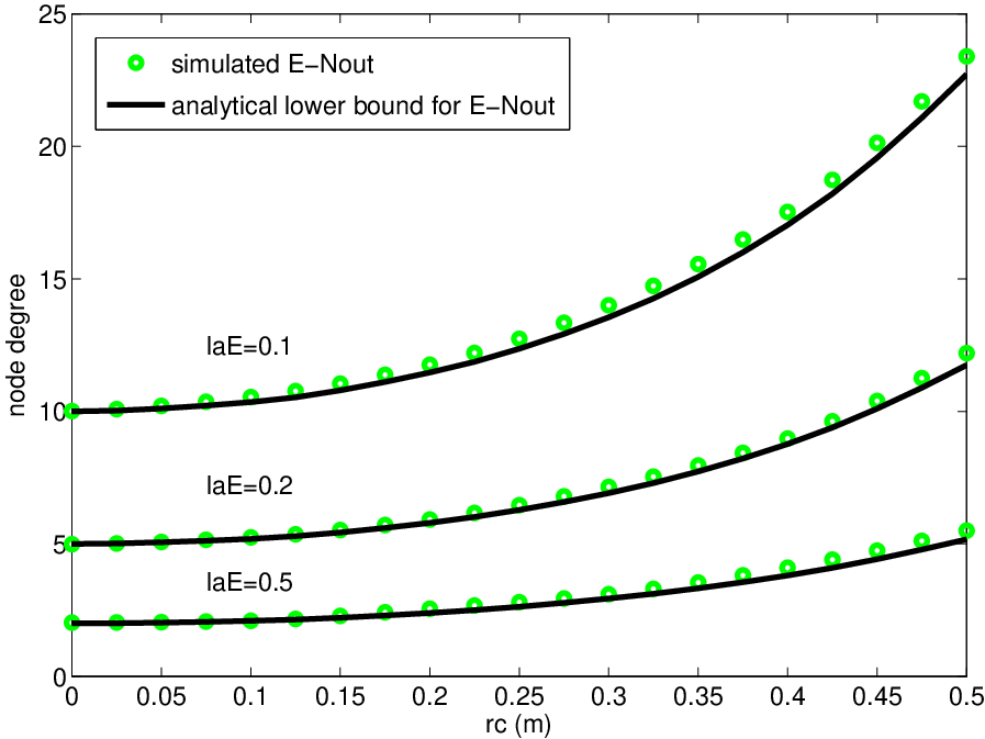
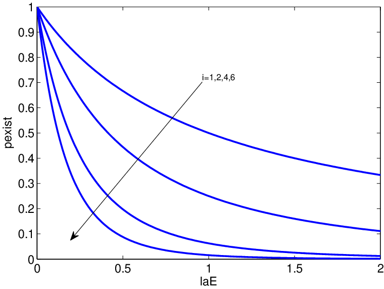
Non-colluding	Colluding
$P_{\textrm{rx},\textrm{e}}=\frac{P_{\mathrm{l}}}{R_{\textrm{e},1}^{2b}}$	$P_{\textrm{rx},\textrm{e}}=\sum_{i=1}^{\infty}\frac{P_{\ell}}{R_{\textrm{e},i}^{2b}}$
$f_{P_{\textrm{rx},\textrm{e}}}(x)=\frac{\pi\lambda_{\textrm{e}}}{bx}\left(\frac{P_{\ell}}{x}\right)^{1/b}\exp\left(-\pi\lambda_{\textrm{e}}\left(\frac{P_{\ell}}{x}\right)^{1/b}\right),x\geq 0$	$P_{\textrm{rx},\textrm{e}}\sim\mathcal{S}\left(\alpha=\frac{1}{b},\>\beta=1,\>\gamma=\pi\lambda_{\textrm{e}}\mathcal{C}_{1/b}^{-1}P_{\ell}^{1/b}\right)$
$F_{\mathpzc{R}_{\mathrm{s}}}(c)=1-\exp\left(-\pi\lambda_{\textrm{e}}\left(\frac{\frac{P_{\ell}}{\sigma_{\textrm{e}}^{2}}}{\left(1+\frac{P_{\ell}}{r_{\ell}^{2b}\sigma_{\ell}^{2}}\right)2^{-\varrho}-1}\right)^{1/b}\right),0\leq\varrho<\mathpzc{R}_{\ell}$	$F_{\mathpzc{R}_{\mathrm{s}}}(c)=1-F_{\widetilde{P}_{\textrm{rx},\textrm{e}}}\left(\frac{\left(1+\frac{P_{\ell}}{r_{\ell}^{2b}\sigma_{\ell}^{2}}\right)2^{-\varrho}-1}{(\pi\lambda_{\textrm{e}}\mathcal{C}_{1/b}^{-1})^{b}\frac{P_{\ell}}{\sigma_{\textrm{e}}^{2}}}\right),0\leq\varrho<\mathpzc{R}_{\ell}$
	with $\widetilde{P}_{\textrm{rx},\textrm{e}}\sim\mathcal{S}\left(\alpha=\frac{1}{b},\>\beta=1,\>\gamma=1\right)$
$p_{\mathrm{exist}}=\exp\left(-\pi\lambda_{\textrm{e}}r_{\ell}^{2}\left(\frac{\sigma_{\ell}^{2}}{\sigma_{\textrm{e}}^{2}}\right)^{1/b}\right)$	$p_{\mathrm{exist}}=F_{\widetilde{P}_{\textrm{rx},\textrm{e}}}\left(\frac{\sigma_{\textrm{e}}^{2}}{(\pi\lambda_{\textrm{e}}r_{\ell}^{2}\mathcal{C}_{1/b}^{-1})^{b}\sigma_{\ell}^{2}}\right)$
$\mathbb{E}\{N_{\mathrm{out}}\}=\frac{\lambda_{\ell}}{\lambda_{\textrm{e}}}$	$\mathbb{E}\{N_{\mathrm{out}}\}=\frac{\lambda_{\ell}}{\lambda_{\textrm{e}}}\,\textrm{sinc}\!\left(\frac{1}{b}\right)$

Table IV: Comparison between the cases of non-colluding and colluding eavesdroppers, considering a single legitimate link, and a channel gain of the form

g(r)=\frac{1}{r^{2b}}

$\displaystyle\mathbb{P}_{x}\{\|x\|<R_{\textrm{e},1}\}$	$\displaystyle=\mathbb{P}_{\Theta,\Pi_{\textrm{e}}}\{\Pi_{\textrm{e}}\{\overline{\Theta}\cap\mathcal{D}(\rho,\|x\|)\backslash\mathcal{B}_{x}(\rho)\}=0\}$	(73)
	$\displaystyle\geq\mathbb{P}_{\Theta,\Pi_{\textrm{e}}}\{\Pi_{\textrm{e}}\{\overline{\Theta}\cap\mathcal{D}(\rho,\|x\|)\}=0\}$	(74)
	$\displaystyle=\mathbb{E}_{\Theta}\{\exp(-\lambda_{\textrm{e}}\mathbb{A}\{\overline{\Theta}\cap\mathcal{D}(\rho,\|x\|)\}\}$	(75)
	$\displaystyle\geq\exp(-\lambda_{\textrm{e}}\mathbb{E}_{\Theta}\{\mathbb{A}\{\overline{\Theta}\cap\mathcal{D}(\rho,\|x\|)\}\}),$	(76)

$\displaystyle\mathbb{E}_{\Theta}\{\mathbb{A}\{\overline{\Theta}\cap\mathcal{D}(\rho,\|x\|)\}\}$	$\displaystyle=\mathbb{E}_{\Theta}\left\{{\int\intop}_{\mathbb{R}^{2}}\mathbbm{1}\{y\in\overline{\Theta}\cap\mathcal{D}(\rho,\|x\|)\}dy\right\}$
	$\displaystyle={\int\intop}_{\mathcal{D}(\rho,\|x\|)}\mathbb{P}\{y\in\overline{\Theta}\}dy$
	$\displaystyle={\int\intop}_{\mathcal{D}(\rho,\|x\|)}\mathbb{P}\{\Pi_{\ell}\{\mathcal{B}_{y}(\rho)\}=0\}dy$
	$\displaystyle={\int\intop}_{\mathcal{D}(\rho,\|x\|)}\underbrace{e^{-\lambda_{\ell}\pi\rho^{2}}}_{\triangleq p_{\overline{\Theta}}}dy$
	$\displaystyle=p_{\overline{\Theta}}\pi(\|x\|^{2}-\rho^{2})$	(77)

Abstract

Index Terms:

I Introduction

II System Model

II-A Wireless Propagation Characteristics

II-B Wireless Information-Theoretic Security

Definition II.1 (Strong Secrecy)

II-C i​𝒮​-i\mathcal{S}\textrm{-}Graph

Definition II.2 (i​𝒮​-i\mathcal{S}\textrm{-}graph)

II-D Poisson i​𝒮​-i\mathcal{S}\textrm{-}Graph

Definition II.3 (Poisson i​𝒮​-i\mathcal{S}\textrm{-}graph)

III Local Connectivity in the Poisson i​𝒮​-i\mathcal{S}\textrm{-}Graph

Property III.1

Proof:

III-A In-Degree Characterization

Theorem III.1

Proof:

Corollary III.1

Proof:

III-B Out-Degree Characterization

Theorem III.2

Proof:

Corollary III.2

Proof:

III-C General Relationships Between In- and Out-Degree

Property III.2

Proof:

Property III.3

Proof:

III-D Effect of the Wireless Propagation Characteristics

Theorem III.3

Proof:

Corollary III.3

Proof:

III-E Effect of the Secrecy Rate Threshold and Noise Powers

Property III.4

Proof:

Theorem III.4

Proof:

III-F Numerical Results

IV Techniques for Communication with Enhanced Secrecy

IV-A Sectorized Transmission

Theorem IV.1

Proof:

Corollary IV.1

Proof:

IV-B Eavesdropper Neutralization

Theorem IV.2

Proof:

IV-C Numerical Results

V Maximum Secrecy Rate in the Poisson i​𝒮​-i\mathcal{S}\textrm{-}Graph

V-A Distribution of the Maximum Secrecy Rate

Theorem V.1

Proof:

V-B Existence and Outage of the Maximum Secrecy Rate

Corollary V.1

Proof:

V-C Numerical Results

VI The Case of Colluding Eavesdroppers

VI-A Maximum Secrecy Rate of a Single Link

Theorem VI.1

Proof:

VI-B Distribution of the Maximum Secrecy Rate of a Single Link

Theorem VI.2

Proof:

VI-C Existence and Outage of the Maximum Secrecy Rate of a Single Link

Corollary VI.1

Proof:

VI-D Colluding vs. Non-Colluding Eavesdroppers for a Single Link

VI-E i​𝒮​-i\mathcal{S}\textrm{-}Graph with Colluding Eavesdroppers

Theorem VI.3

Proof:

VI-F Numerical Results

VII Conclusions

Appendix A Proof that Inequality (23) is Strict

Appendix B Derivation of (45)

Appendix C Derivation of (68)

Acknowledgements

References

II-C $i\mathcal{S}\textrm{-}$ Graph

Definition II.2 ( $i\mathcal{S}\textrm{-}$ graph)

II-D Poisson $i\mathcal{S}\textrm{-}$ Graph

Definition II.3 (Poisson $i\mathcal{S}\textrm{-}$ graph)

III Local Connectivity in the Poisson $i\mathcal{S}\textrm{-}$ Graph

V Maximum Secrecy Rate in the Poisson $i\mathcal{S}\textrm{-}$ Graph

VI-E $i\mathcal{S}\textrm{-}$ Graph with Colluding Eavesdroppers