跳到论文正文
W Papers独立论文阅读器 arXiv:1001.3665 论文正文 计算阅读时间 · 0%
引用这篇论文根据当前论文元数据生成,正式投稿前建议核对。


License: arXiv.org perpetual non-exclusive license
arXiv:1001.3665v4 [math.AP] 31 May 2010

Adiabatic evolution of 1D shape resonances: an artificial interface conditions approach.

A. Faraj*    A. Mantile*    F. Nier Note: IRMAR, UMR - CNRS 6625, Université Rennes 1, Campus de Beaulieu, 35042 Rennes Cedex, France
Abstract

Artificial interface conditions parametrized by a complex number θ0\theta_{0} are introduced for 1D-Schrödinger operators. When this complex parameter equals the parameter θ∈i​ℝ\theta\in i\mathbb{R} of the complex deformation which unveils the shape resonances, the Hamiltonian becomes dissipative. This makes possible an adiabatic theory for the time evolution of resonant states for arbitrarily large time scales. The effect of the artificial interface conditions on the important stationary quantities involved in quantum transport models is also checked to be as small as wanted, in the polynomial scale (hN)N∈ℕ(h^{N})_{N\in\mathbb{N}} as h→0h\to 0, according to θ0\theta_{0}.

1 Introduction

The adiabatic evolution of resonances is an old problem which has received various answers in the last twenty years. The most effective results where obtained by remaining on the real spectrum and by considering the evolution of quasi-resonant states (see for example [48][60][1]). Motivated by nonlinear problems coming from the modelling of quantum electronic transport, we reconsider this problem and propose a new approach which rely on a modification of the initial kinetic energy operator −h2​Δ-h^{2}\Delta into −h2​Δθ0h-h^{2}\Delta_{\theta_{0}}^{h} where θ0\theta_{0} parametrizes artificial interface conditions. With this analysis, we aim at developing reduced models for the nonlinear dynamics of transverse quantum transport in resonant tunneling diodes or possibly more complex structures. A functional framework for such a model has been proposed in [45] and implements a dynamically nonlinear version of the Landauer-Büttiker approach based on Mourre’s theory and Sigal-Soffer propagation estimates (see [16] and [15] for an alternative presentation of the stationary problem). The derivation of reduced models for the steady state problem has been developed in [20][21][46] on the basis of Helffer-Sjöstrand analysis of resonances in [30]. This asymptotic model elucidated the influence of the geometry of the potential on the feasibility of hysteresis phenomena already studied in [33][50]. Numerical applications have been carried out in realistic G​a−A​sGa-As or S​i−S​i​O2Si-SiO_{2} structure in [19] and [18], showing a good agreement with previous numerical simulations in [17] or [41] and finally predicting the possibility of exotic bifurcation diagrams. From the modelling point of view a difficulty comes from the phase-space description of the tunnel effect which can be summarized with the importance in the asymptotic nonlinear system of the asymptotic value of the branching ratio

tj=limh→0|⟨Whψ~h−(+k,.),Φjh⟩|24​h​k​Γjh.t_{j}=\lim_{h\to 0}\frac{|\langle W^{h}\widetilde{\psi}^{h}_{-}(+k,.)\,,\,\Phi_{j}^{h}\rangle|^{2}}{4hk\Gamma_{j}^{h}}\,. (1.1)

In the above formula zjh=Ejh−i​Γjhz_{j}^{h}=E_{j}^{h}-i\Gamma_{j}^{h} is a resonance for the Hamiltonian Hh=−h2​Δ+V−WhH^{h}=-h^{2}\Delta+V-W^{h} with a semiclassical island VV and a quantum well WhW^{h}, ψ~−(±k,.)\tilde{\psi}_{-}(\pm k,.) are the generalized eigenfunctions for the filled well Hamiltonian H~h=−h2​Δ+V\widetilde{H}^{h}=-h^{2}\Delta+V with a momentum ±k\pm k such that k2∼Ejhk^{2}\sim E_{j}^{h} and Φjh\Phi_{j}^{h} is the jj-th eigenfunction of the Dirichlet Hamiltonian HDh=−h2​Δ+V−WhH^{h}_{D}=-h^{2}\Delta+V-W^{h} on some finite interval (a,b)(a,b). The imaginary part of the resonance is given by the Fermi Golden rule proved in [21]

Γjh​(1+o⁡(1))=|⟨Wh​ψ~−h​(+k,⋅),ϕjh⟩|24​h​k+|⟨Wh​ψ~−h​(−k,⋅),ϕjh⟩|24​h​k,\Gamma_{j}^{h}(1+o(1))=\frac{|\langle W^{h}\tilde{\psi}^{h}_{-}(+k,\cdot),\phi^{h}_{j}\rangle|^{2}}{4hk}+\frac{|\langle W^{h}\tilde{\psi}^{h}_{-}(-k,\cdot),\phi^{h}_{j}\rangle|^{2}}{4hk}\,, (1.2)

where the interaction with the continuous spectrum leading to a resonance contains two contributions from the left-hand side with +k+k and from the right-hand side with −k-k.

Our purpose is the derivation of reduced models for the dynamics of quantum nonlinear systems like it has been done in the stationary case in [20][21][46] with the following motto: The (nonlinear) phenomena are governed by a finite number of resonant states. As this was already explained in [20], such a remark dictates the scaling of the potential which leads to the small parameter analysis and in the end to effective reduced models even when h∼0.1h\sim 0.1 or 0.30.3 (see [19]).
For the dynamical problem, the time evolution of resonant states have to be considered possibly with a time-dependent potential. And it is known that this is a rather subtle point. Quantum resonances follow almost but not exactly the general intuition (see [53]) and remain an inexhaustible playground for mathematical analysis. For example, the exponential decay law is an approximation which has a physical interpretation in terms of the evolution of quasi-resonant states (truncated resonant states which lie on the real L2L^{2}-space) and writes as

e−i​t​Hh​ψq​r,j=e−i​t​Ej​e−t​Γj​ψq​r,j+R⁡(t),e^{-itH^{h}}\psi_{qr,j}=e^{-itE_{j}}e^{-t\Gamma_{j}}\psi_{qr,j}+R(t)\,,

where the remainder term R⁡(t)R(t) is small only in the range of times scaled as 1Γj\frac{1}{\Gamma_{j}}. A very accurate analysis of this has been done in [27][57][58][59][39][38] and adiabatic results for slowly varying potentials and for quasi-resonant states have been obtained in [48](see also [60] and [1] in a similar spirit) on this range of time-scales. On the other side the relation

e−i​t​Hh​(θ)​ψj=e−i​t​Ej​e−t​Γj​ψje^{-itH^{h}(\theta)}\psi_{j}=e^{-itE_{j}}e^{-t\Gamma_{j}}\psi_{j}

holds without remainder terms when θ∈i​ℝ+\theta\in i\mathbb{R}_{+} parametrizes a complex deformation of HhH^{h} according to the general approach to resonances (see [3][10][31][23][30][29]). However, and this is well known within the analysis of resonances, the deformed generator i​Hh​(θ)iH^{h}(\theta) is not maximal accretive although its spectrum lies in {Rez≥0}\left\{\mathop{\mathrm{Re}}~z\geq 0\right\} and no uniform estimates are available on e−i​t​Hh​(θ)e^{-itH^{h}(\theta)} . One of the two next strategies have to be chosen:

  • •

    Stay on the real space with quasi-resonant states, with uniform estimates of the semigroups, groups or dynamical systems (they are unitary) but with remainder term which can be neglected only on some parameter dependent range of time.

  • •

    Consider the complex deformed situation and try to solve or bypass the defect of accretivity.

Because the remainder terms seemed hard to handle within the original nonlinear problem and also because there may be multiple time scales to handle, due to the nonlinearity or due to several resonances involved in the nonlinear process, we chose the second one.

In a one dimensional problem the simplest approach is the complex dilation method according to [3][10][23]. Since the possibly nonlinear potential with a compact support has a limited regularity inside the interval (a,b)(a,b), this deformation is done only outside this interval following an approach already presented in [54]. The dilation is defined according to

Uθ​ψ​(x)={eθ2​ψ​(eθ​(x−b)+b),x>bψ⁡(x),x∈(a,b)eθ2​ψ​(eθ​(x−a)+a),x<a,U_{\theta}\psi(x)=\left\{\begin{array}[c]{ll}e^{\frac{\theta}{2}}\psi(\vskip 3.0pt plus 1.0pt minus 1.0pte^{\theta}(x-b)+b),&x>b\\ \vskip 3.0pt plus 1.0pt minus 1.0pt\psi(x),&x\in(a,b)\\ e^{\frac{\theta}{2}}\psi(\vskip 3.0pt plus 1.0pt minus 1.0pte^{\theta}(x-a)+a),&x<a\,,\end{array}\right. (1.3)

and finally handled with θ∈i​ℝ+\theta\in i\mathbb{R}_{+}. The conjugated Laplacian is

Uθ​(−h2​Δ)​Uθ−1=−h2​e−2​θ​ 1ℝ∖(a,b)​(x)​Δ,U_{\theta}(-h^{2}\Delta)U_{\theta}^{-1}=-h^{2}e^{-2\theta\,1_{\mathbb{R}\setminus(a,b)}(x)}\Delta\,,

with the domain made of functions u∈H2​(ℝ∖{a,b})u\in H^{2}(\mathbb{R}\setminus\left\{a,b\right\}) with the interface conditions

[e−θ2​u​(b+)=u⁡(b−);e−3​θ2​u′​(b+)=u′​(b−)e−θ2u(a−)=u(a+);e−3​θ2u′(a−)=u′(a+).\left[\begin{array}[c]{l}e^{-\frac{\theta}{2}}u(b^{+})=u(b^{-});\quad\vskip 6.0pt plus 2.0pt minus 2.0pte^{-\frac{3\theta}{2}}u^{\prime}(b^{+})=u^{\prime}(b^{-})\\ e^{-\frac{\theta}{2}}u(a^{-})=u(a^{+});\quad e^{-\frac{3\theta}{2}}u^{\prime}(a^{-})=u^{\prime}(a^{+})\,.\end{array}\right. (1.4)

This can be viewed as a singular version of the black-box formalism of [56]. Additionally to the fact that this singular deformation is convenient for the original model with potential barriers presented with a discontinuous potential and with a nonlinear part inside (a,b)(a,b), the obstruction to the accretivity of Uθ​(−h2​Δ)​Uθ−1U_{\theta}(-h^{2}\Delta)U_{\theta}^{-1} is concentrated in two boundary terms at x=ax=a and x=bx=b in

Re⟨u,i​Uθ​(−h2​Δ)​Uθ−1​u⟩L2​(ℝ)=Re[i​h2​(u¯​u′)|a−b+​(e−2​θ−e−θ¯+3​θ2)]+h2e−2Reθsin(2Imθ)∫ℝ∖[a,b]|u′|2dx.\mathop{\mathrm{Re}}~\langle u\,,\,iU_{\theta}(-h^{2}\Delta)U_{\theta}^{-1}u\rangle_{L^{2}(\mathbb{R})}=\mathop{\mathrm{Re}}~\left[ih^{2}(\bar{u}u^{\prime})\big|_{a^{-}}^{b^{+}}(e^{-2\theta}-e^{-\frac{\bar{\theta}+3\theta}{2}})\right]\\ +h^{2}e^{-2\mathop{\mathrm{Re}}~\theta}\sin(2\mathop{\mathrm{Im}}~\theta)\int_{\mathbb{R}\setminus[a,b]}|u^{\prime}|^{2}~dx\,. (1.5)

Our strategy then relies on the introduction of artificial interface conditions parametrized with θ0\theta_{0} which modify the operator −h2​Δ-h^{2}\Delta. The parameter θ0\theta_{0} is then chosen so that the above boundary term vanishes when θ=θ0=i​τ\theta=\theta_{0}=i\tau. The modified and deformed Hamiltonian Hθ0=i​τh​(θ=i​τ)H^{h}_{\theta_{0}=i\tau}(\theta=i\tau) then generates a contraction semigroup and uniform estimates are available for e−i​t​Hi​τ​(i​τ)e^{-itH_{i\tau}(i\tau)} or for the dynamical system (Uh​(t,s))t≥s(U^{h}(t,s))_{t\geq s} for time-dependent potentials .
Hopefully this modification has a little effect on the Hamiltonian Hh=−h2​Δ+V−WhH^{h}=-h^{2}\Delta+V-W^{h} and all the quantities involved in the nonlinear problem, with explicit estimates with respect to θ0\theta_{0} and hh. Indeed all the quantities and even the exponentially small ones like Γj\Gamma_{j} or the ones appearing in the branching ratio (1.1) experiment small relative variation with respect to θ0\theta_{0} when θ0=i​hN0\theta_{0}=ih^{N_{0}} with N0≥5N_{0}\geq 5.
In comparison with the modelling of artificial dissipative boundary conditions in [11][12][13][14], our approach has the advantage of remaining close to the initial quantum model. Such a comparison is valuable and ensures the validity of numerical applications when the non-linear bifurcation phenomena are very sensitive to small variations of the data.
Once the above comparison is done, it is checked that adiabatic evolution for a slowly varying potential or equivalently for the ε\varepsilon-dependent Cauchy problem

i​ε​∂tu=Hθ0h​(θ0,t)​u,ut=0=u0,i\varepsilon\partial_{t}u=H_{\theta_{0}}^{h}(\theta_{0},t)u\,,\quad u_{t=0}=u_{0}\,,

with some exponentially large time scale 1ε=eCh\frac{1}{\varepsilon}=e^{\frac{C}{h}}, is adapted from the general approach for the adiabatic evolution of bound states of self-adjoint generators in [8][43][34].
Adiabatic dynamics have already been considered within the modelling of out-of-equilibrium quantum transport in [22][7][9] playing with the continuous spectrum with self-adjoint techniques. Only partial results are known with non self-adjoint generators: in [42] only small time results are valid for resonances, in [44] bounded generators are considered and in [55] a general scheme for the the higher order construction of the adapted projector is done but without time propagation estimates. In [35], A. Joye considered a general time-adiabatic evolution for semigroups in Banach spaces under a fixed gap condition and with analyticity assumptions: The exponential growth of the dynamical system ‖Sε​(t,0)‖≤eC​tε\|S_{\varepsilon}(t,0)\|\leq e^{\frac{Ct}{\varepsilon}} is compensated by the 𝒪⁡(e−cε){\cal O}(e^{-\frac{c}{\varepsilon}}) error of the adiabatic approximation under analyticity assumptions (see [43][34]) and lead to a total error 𝒪⁡(C​t−cε)\mathcal{O}(\frac{Ct-c}{\varepsilon}) which is small when t<c/Ct<c/C. Our adaptation combines the uniform estimates due to the accretivity of the modified and deformed Hamiltonian with the accurate resolvent estimate provided by the accurate comparison with self-adjoint problems (shape resonances result from the coupling of some Dirichlet eigenvalues with a continuous spectrum). Although, the error associated with the adiabatic evolution is estimated at the first order as an 𝒪⁡(ε1−δ)\mathcal{O}(\varepsilon^{1-\delta}), with δ>0\delta>0 as small as wanted, it is necessary to reconsider the higher-order method in [43] or [34], because we work with small gaps (vanishing as h→0h\to 0) and with non self-adjoint operators. Finally note that the exponential time scale is not necessarily related with the imaginary parts of resonances and several resonant states with various life-time scales are taken into account in our application.

The outline of the article is the following.

  • •

    The artificial interface conditions parametrized by θ0\theta_{0} are introduced in Section 2. With these new interface conditions −Δ-\Delta is transformed into a non self-adjoint operator conjugated with −Δ-\Delta, W⁡(θ0)​(−Δ)​W​(θ0)−1W(\theta_{0})(-\Delta)W(\theta_{0})^{-1} with W(θ0)=IdL2+𝒪(θ0)W(\theta_{0})=\mathop{\mathrm{Id}\,}_{L^{2}}+\mathcal{O}(\theta_{0}). The case with a potential is illustrated with numerical computations.

  • •

    The functional analysis of the complex deformation parametrized with θ\theta is done in Section 3. After introducing a Krein formula associated with the (θ0,θ)(\theta_{0},\theta)-dependent interface conditions, it mimics the standard approach to resonances summarized in [23][29] but things have to be reconsidered for we start from an already non self-adjoint operator when θ0≠0\theta_{0}\neq 0. Assumptions on the time-dependent variations of the potential which ensure the well-posedness of the dynamical systems are specified in the end of this section.

  • •

    The small parameter problem modelling quantum wells in a semiclassical island is introduced in Section 4. Accurate exponential decay estimates are presented for the spectral problems reduced to (a,b)(a,b) making use of the fact that our operators are proportional to −h2​Δ-h^{2}\Delta outside [a,b][a,b].

  • •

    The Grushin problem leading to an accurate theory of resonances is presented in Section 5. There it is checked that the imaginary parts of the resonances, which are exponentially small, are little perturbed by the introduction of θ0\theta_{0}-dependent artificial conditions. The conclusion of this section is that all the quantities involved in the Fermi Golden Rule (1.2) have little relative variations with respect to θ0\theta_{0}, even the exponentially small ones.

  • •

    Accurate parameter-dependent resolvent estimates for the whole space problem are done in Section 6. Again the Krein formula for the resolvent associated with the (θ0,θ)(\theta_{0},\theta)-dependent interface conditions is especially useful.

  • •

    The adiabatic evolution of resonances is really introduced in 7. After specifying all the assumptions, the main result about this is stated in Theorem 7.1.

  • •

    The appendix contains various preliminary and sometimes well-known estimates, plus a variation of the general adiabatic theory concerned with non self-adjoint maximal accretive operators in Section B

2 Artificial interface conditions

Modified Hamiltonians with artificial interface conditions are introduced. It is checked that the effect of these artificial conditions parametrized by θ0∈ℂ\theta_{0}\in\mathbb{C} is of order |θ0||\theta_{0}| for all the quantities associated with the free Schrödinger Hamiltonian −h2​Δ-h^{2}\Delta on the whole line. Instead of pursuing this analysis for general Schrödinger operators −h2​Δ+V-h^{2}\Delta+V we simply give a numerical evidence of this stability with respect θ0\theta_{0} .

2.1 The modified Laplacian

We consider a class of singular perturbations of the 1-D Laplacian, defined through non self-adjoint boundary conditions in the extrema of a bounded interval. For θ0∈ℂ\theta_{0}\in\mathbb{C} and a,b∈ℝa,b\in\mathbb{R}, with a<ba<b and b−a=Lb-a=L, the Hamiltonian Hθ0,0hH_{\theta_{0},0}^{h} is defined by

{D⁡(Hθ0,0h)={u∈H2​(ℝ\{a,b}):[e−θ02​u​(b+)=u⁡(b−);e−32​θ0​u′​(b+)=u′​(b−)e−θ02​u​(a−)=u⁡(a+);e−32​θ0​u′​(a−)=u′​(a+)},Hθ0,0hu=−h2∂x2,\left\{\begin{array}[c]{l}\vskip 6.0pt plus 2.0pt minus 2.0ptD(H_{\theta_{0},0}^{h})=\left\{u\in H^{2}(\mathbb{R}\backslash\left\{a,b\right\}):\left[\begin{array}[c]{l}\vskip 3.0pt plus 1.0pt minus 1.0pte^{-\frac{\theta_{0}}{2}}u(b^{+})=u(b^{-});\ e^{-\frac{3}{2}\theta_{0}}u^{\prime}(b^{+})=u^{\prime}(b^{-})\\ e^{-\frac{\theta_{0}}{2}}u(a^{-})=u(a^{+});\ e^{-\frac{3}{2}\theta_{0}}u^{\prime}(a^{-})=u^{\prime}(a^{+})\end{array}\right.\right\}\,,\\ H_{\theta_{0},0}^{h}u=-h^{2}\partial_{x}^{2}\,,\end{array}\right. (2.1)

where u⁡(x+)u(x^{+}) and u⁡(x−)u(x^{-}) respectively denote the right and the left limits of uu in xx, while the notation u′u^{\prime} is used for the first derivative. When |θ0|\left|\theta_{0}\right| is small, the analysis of Hθ0,0hH_{\theta_{0},0}^{h} follows by a direct comparison with H0,0hH_{0,0}^{h} (coinciding with the usual Laplacian: −h2​Δℝ-h^{2}\Delta_{\mathbb{R}}). To fix this point, let us introduce the intertwining operator Wθ0W_{\theta_{0}} defined through the integral kernel

Wθ0​(x,y)=∫−∞+∞ψ−​(k,x)​e−i​kh​y​d​k2​π​h,W_{\theta_{0}}(x,y)=\int_{-\infty}^{+\infty}\psi_{-}(k,x)e^{-i\frac{k}{h}y}~\frac{dk}{2\pi h}\,, (2.2)

with ψ−​(k,x)\psi_{-}(k,x) denoting the generalized eigenfunctions associated with our model. These are described by the plane wave solutions to the equation

(Hθ0,0h−k2)​ψ−​(k,⋅)=0.\left(H_{\theta_{0},0}^{h}-k^{2}\right)\psi_{-}(k,\cdot)=0\,. (2.3)

For k>0k>0, one has

1(0,+∞)​(k)​ψ−​(k,x)={ei​kh​x+R⁡(k)​e−i​kh​x,x<aA⁡(k)​ei​kh​x+B⁡(k)​e−i​kh​x,x∈(a,b)T⁡(k)​ei​kh​x,x>b.1_{(0,+\infty)}(k)\,\psi_{-}(k,x)=\left\{\begin{array}[c]{ll}\vskip 6.0pt plus 2.0pt minus 2.0pte^{i\frac{k}{h}x}+R(k)e^{-i\frac{k}{h}x},&x<a\\ \vskip 6.0pt plus 2.0pt minus 2.0ptA(k)e^{i\frac{k}{h}x}+B(k)e^{-i\frac{k}{h}x},&x\in(a,b)\\ T(k)e^{i\frac{k}{h}x},&x>b\,.\end{array}\right. (2.4)

Since ψ−​(k,x)\psi_{-}(k,x) fulfills the boundary conditions in (2.1), the explicit expression of the coefficients in (2.4) are

{A(k)=2c+​(θ0)​e−i​kh​Ld⁡(θ0,k),B(k)=−2c−​(θ0)​e2​i​kh​a​ei​kh​Ld⁡(θ0,k),T(k)=e−i​kh​Ld⁡(θ0,k)(c+(θ0)2−c−(θ0)2),R(k)=−2​i​c+​(θ0)​c−​(θ0)d⁡(θ0,k)e2​i​kh​asin(k​Lh),\left\{\begin{array}[c]{l}\vskip 6.0pt plus 2.0pt minus 2.0ptA(k)=2\frac{c_{+}(\theta_{0})e^{-i\frac{k}{h}L}}{d(\theta_{0},k)}\,,\qquad B(k)=-2\frac{c_{-}(\theta_{0})e^{2i\frac{k}{h}a}e^{i\frac{k}{h}L}}{d(\theta_{0},k)}\,,\\ T(k)=\frac{e^{-i\frac{k}{h}L}}{d(\theta_{0},k)}\left(c_{+}(\theta_{0})^{2}-c_{-}(\theta_{0})^{2}\right)\,,\qquad R(k)=\frac{-2ic_{+}(\theta_{0})c_{-}(\theta_{0})}{d(\theta_{0},k)}e^{2i\frac{k}{h}a}\sin\left(\frac{kL}{h}\right)\,,\end{array}\right. (2.5)

with: c+​(θ0)=eθ02+e32​θ0c_{+}(\theta_{0})=e^{\frac{\theta_{0}}{2}}+e^{\frac{3}{2}\theta_{0}}, c−​(θ0)=eθ02−e32​θ0c_{-}(\theta_{0})=e^{\frac{\theta_{0}}{2}}-e^{\frac{3}{2}\theta_{0}} and

d⁡(θ0,k)=det(c+​(θ0)​ei​kh​ac−​(θ0)​e−i​kh​ac−​(θ0)​ei​kh​bc+​(θ0)​e−i​kh​b)=c+​(θ0)2​e−i​kh​L−c−​(θ0)2​ei​kh​L.d(\theta_{0},k)=\det\begin{pmatrix}c_{+}(\theta_{0})e^{i\frac{k}{h}a}&c_{-}(\theta_{0})e^{-i\frac{k}{h}a}\\ c_{-}(\theta_{0})e^{i\frac{k}{h}b}&c_{+}(\theta_{0})e^{-i\frac{k}{h}b}\end{pmatrix}=c_{+}(\theta_{0})^{2}e^{-i\frac{k}{h}L}-c_{-}(\theta_{0})^{2}e^{i\frac{k}{h}L}\,. (2.6)

For k<0k<0, an analogous computation gives

1(−∞,0)​(k)​ψ−​(k,x)={T~​(k)​ei​kh​x,x<aA~​(k)​ei​kh​x+B~​(k)​e−i​kh​x,x∈(a,b)ei​kh​x+R~​(k)​e−i​kh​x,x>b,1_{(-\infty,0)}(k)\,\psi_{-}(k,x)=\left\{\begin{array}[c]{ll}\vskip 6.0pt plus 2.0pt minus 2.0pt\tilde{T}(k)e^{i\frac{k}{h}x},&x<a\\ \vskip 6.0pt plus 2.0pt minus 2.0pt\tilde{A}(k)e^{i\frac{k}{h}x}+\tilde{B}(k)e^{-i\frac{k}{h}x},&x\in(a,b)\\ e^{i\frac{k}{h}x}+\tilde{R}(k)e^{-i\frac{k}{h}x},&x>b\,,\end{array}\right. (2.7)

with

{A~​(k)=A​(−k),B~​(k)=e4​i​kh​a​e2​i​kh​L​B​(−k),T~​(k)=T​(−k),R~​(k)=e4​i​kh​a​e2​i​kh​L​R​(−k).\left\{\begin{array}[c]{ll}\vskip 6.0pt plus 2.0pt minus 2.0pt\tilde{A}(k)=A(-k)\,,&\tilde{B}(k)=e^{4i\frac{k}{h}a}e^{2i\frac{k}{h}L}B(-k)\,,\\ \tilde{T}(k)=T(-k)\,,&\tilde{R}(k)=e^{4i\frac{k}{h}a}e^{2i\frac{k}{h}L}R(-k)\,.\end{array}\right. (2.8)

In what follows we adopt the simplified notation

A⁡(k,θ0)={A⁡(k),k≥0A~​(k),k<0,B⁡(k,θ0)={B⁡(k),k≥0B~​(k)k<0,A(k,\theta_{0})=\left\{\begin{array}[c]{ll}A(k),&k\geq 0\\ \tilde{A}(k),&k<0\,,\end{array}\right.\quad B(k,\theta_{0})=\left\{\begin{array}[c]{ll}B(k),&k\geq 0\\ \tilde{B}(k)&k<0\,,\end{array}\right. (2.9)

and

T⁡(k,θ0)={T⁡(k),k≥0T~​(k),k<0,R⁡(k,θ0)={R⁡(k),k≥0R~​(k),k<0.T(k,\theta_{0})=\left\{\begin{array}[c]{ll}T(k),&k\geq 0\\ \tilde{T}(k),&k<0\,,\end{array}\right.\quad R(k,\theta_{0})=\left\{\begin{array}[c]{ll}R(k),&k\geq 0\\ \tilde{R}(k),&k<0\,.\end{array}\right. (2.10)
Lemma 2.1.

The operator Wθ0W_{\theta_{0}} defined by (2.2) verifies the expansion

Wθ0−I​d=𝒪⁡(|θ0|)W_{\theta_{0}}-Id=\mathcal{O}(|\theta_{0}|) (2.11)

in operator norm.

Proof: According to (2.4), (2.7) and to the definition (2.2), one can express the integral kernel Wθ0​(x,y)W_{\theta_{0}}(x,y) as follows

Wθ0​(x,y)=∫−∞+∞ei​kh​(x−y)​d​k2​π​h+1(a,b)(x)∫−∞+∞(A(k,θ0)−1)ei​kh​(x−y)d​k2​π​h+1(a,b)(x)∫−∞+∞B(k,θ0)e−i​kh​(x+y)d​k2​π​h+1(−∞,a)(x)∫−∞0(T(k,θ0)−1)ei​kh​(x−y)d​k2​π​h+1(b,+∞)(x)∫0+∞(T(k,θ0)−1)ei​kh​(x−y)d​k2​π​h+1(b,+∞)(x)∫−∞0R(k,θ0)e−i​kh​(x+y)d​k2​π​h+1(−∞,a)(x)∫0+∞R(k,θ0)e−i​kh​(x+y)d​k2​π​h.W_{\theta_{0}}(x,y)=\int_{-\infty}^{+\infty}e^{i\frac{k}{h}(x-y)}\frac{dk}{2\pi h}\\ +1_{(a,b)}(x)\int_{-\infty}^{+\infty}\left(A(k,\theta_{0})-1\right)e^{i\frac{k}{h}(x-y)}\frac{dk}{2\pi h}+1_{(a,b)}(x)\int_{-\infty}^{+\infty}B(k,\theta_{0})e^{-i\frac{k}{h}(x+y)}\frac{dk}{2\pi h}\\ +1_{(-\infty,a)}(x)\int_{-\infty}^{0}\left(T(k,\theta_{0})-1\right)e^{i\frac{k}{h}(x-y)}\frac{dk}{2\pi h}+1_{(b,+\infty)}(x)\int_{0}^{+\infty}\left(T(k,\theta_{0})-1\right)e^{i\frac{k}{h}(x-y)}\frac{dk}{2\pi h}\\ +1_{(b,+\infty)}(x)\int_{-\infty}^{0}R(k,\theta_{0})e^{-i\frac{k}{h}(x+y)}\frac{dk}{2\pi h}+1_{(-\infty,a)}(x)\int_{0}^{+\infty}R(k,\theta_{0})e^{-i\frac{k}{h}(x+y)}\frac{dk}{2\pi h}\,.

The previous expression is rewritten in terms of operators:

Wθ0−I​d=1(a,b)​ℱ−1​(A⁡(k,θ0)−1)​ℱ+1(a,b)​P​ℱ−1​B​(k,θ0)​ℱ+1(−∞,a)​ℱ−1​1(−∞,0)​(T⁡(k,θ0)−1)​ℱ+1(b,+∞)​ℱ−1​1(0,+∞)​(T⁡(k,θ0)−1)​ℱ+1(b,+∞)​P​ℱ−1​1(−∞,0)​R​(k,θ0)​ℱ+1(−∞,a)​P​ℱ−1​1(0,+∞)​R​(k,θ0)​ℱ,W_{\theta_{0}}-Id=1_{(a,b)}\mathcal{F}^{-1}\left(A(k,\theta_{0})-1\right)\mathcal{F}+1_{(a,b)}P\mathcal{F}^{-1}B(k,\theta_{0})\mathcal{F}\\ +1_{(-\infty,a)}\mathcal{F}^{-1}1_{(-\infty,0)}\left(T(k,\theta_{0})-1\right)\mathcal{F}+1_{(b,+\infty)}\mathcal{F}^{-1}1_{(0,+\infty)}\left(T(k,\theta_{0})-1\right)\mathcal{F}\\ +1_{(b,+\infty)}P\mathcal{F}^{-1}1_{(-\infty,0)}R(k,\theta_{0})\mathcal{F}+1_{(-\infty,a)}P\mathcal{F}^{-1}1_{(0,+\infty)}R(k,\theta_{0})\mathcal{F}\,,

where ℱ\mathcal{F} denotes the Fourier transform normalized as ℱ​u​(k)=∫ℝu⁡(x)​e−i​kh​x​d​x(2​π​h)1/2\mathcal{F}u(k)=\int_{\mathbb{R}}u(x)e^{-i\frac{k}{h}x}\frac{dx}{(2\pi h)^{1/2}}, and PP denotes the parity operator: P​u​(x)=u⁡(−x)Pu(x)=u(-x).
Since the operators PP, ℱ\mathcal{F}, ℱ−1\mathcal{F}^{-1} and multiplication by the characteristic function of a set are uniformly bounded with respect to θ0\theta_{0}, we get:

‖Wθ0−I​d‖≤C⁡(‖A⁡(k,θ0)−1‖L∞​(ℝ)+‖B⁡(k,θ0)‖L∞​(ℝ)+‖T⁡(k,θ0)−1‖L∞​(ℝ)+‖R⁡(k,θ0)‖L∞​(ℝ)).\|W_{\theta_{0}}-Id\|\leq C\left(\|A(k,\theta_{0})-1\|_{L^{\infty}(\mathbb{R})}+\|B(k,\theta_{0})\|_{L^{\infty}(\mathbb{R})}+\|T(k,\theta_{0})-1\|_{L^{\infty}(\mathbb{R})}+\|R(k,\theta_{0})\|_{L^{\infty}(\mathbb{R})}\right)\,.

From (2.8), it is enough to estimate for k>0k>0 the terms at the r.h.s of the inequality above to get the L∞​(ℝ)L^{\infty}(\mathbb{R}) bounds. Moreover, from the definition of the coefficients c−​(θ0)c_{-}(\theta_{0}), c+​(θ0)c_{+}(\theta_{0}) and d⁡(θ0,k)d(\theta_{0},k), we have:

c−​(θ0)=𝒪⁡(|θ0|),c+​(θ0)=2+𝒪⁡(|θ0|),d⁡(θ0,k)=4​e−i​k​Lh+𝒪⁡(|θ0|),c_{-}(\theta_{0})=\mathcal{O}(|\theta_{0}|),\quad c_{+}(\theta_{0})=2+\mathcal{O}(|\theta_{0}|),\quad d(\theta_{0},k)=4e^{-\frac{ikL}{h}}+\mathcal{O}(|\theta_{0}|)\,,

where the upper bound of 𝒪⁡(|θ0|)\mathcal{O}(|\theta_{0}|) holds with a universal constant. The previous equation gives |d⁡(θ0,k)|≥1|d(\theta_{0},k)|\geq 1 when |θ0||\theta_{0}| is small enough, and using (2.5), this implies:

|A⁡(k,θ0)−1|=|2​c+​(θ0)​e−i​k​Lh−d⁡(θ0,k)||d⁡(θ0,k)|=|𝒪⁡(|θ0|)||d⁡(θ0,k)|≤C​|θ0|,|A(k,\theta_{0})-1|=\frac{\left|2c_{+}(\theta_{0})e^{-\frac{ikL}{h}}-d(\theta_{0},k)\right|}{\left|d(\theta_{0},k)\right|}=\frac{\left|\mathcal{O}(|\theta_{0}|)\right|}{\left|d(\theta_{0},k)\right|}\leq C|\theta_{0}|\,,
|T⁡(k,θ0)−1|=|e−i​k​Lh​(c+​(θ0)2−c−​(θ0)2)−d⁡(θ0,k)||d⁡(θ0,k)|=|2​c−​(θ0)2​sin⁡(k​Lh)||d⁡(θ0,k)|=|𝒪⁡(|θ0|2)||d⁡(θ0,k)|≤C​|θ0|,|T(k,\theta_{0})-1|=\frac{\left|e^{-\frac{ikL}{h}}\left(c_{+}(\theta_{0})^{2}-c_{-}(\theta_{0})^{2}\right)-d(\theta_{0},k)\right|}{\left|d(\theta_{0},k)\right|}=\frac{\left|2c_{-}(\theta_{0})^{2}\sin\left(\frac{kL}{h}\right)\right|}{\left|d(\theta_{0},k)\right|}=\frac{\left|\mathcal{O}(|\theta_{0}|^{2})\right|}{\left|d(\theta_{0},k)\right|}\leq C|\theta_{0}|\,,
|B⁡(k,θ0)|=|2​c−​(θ0)||d⁡(θ0,k)|=|𝒪⁡(|θ0|)||d⁡(θ0,k)|≤C​|θ0|,|B(k,\theta_{0})|=\frac{\left|2c_{-}(\theta_{0})\right|}{\left|d(\theta_{0},k)\right|}=\frac{\left|\mathcal{O}(|\theta_{0}|)\right|}{\left|d(\theta_{0},k)\right|}\leq C|\theta_{0}|\,,
|R⁡(k,θ0)|=|2​c+​(θ0)​c−​(θ0)​sin⁡(k​Lh)||d⁡(θ0,k)|=|(2+𝒪⁡(|θ0|))​𝒪​(|θ0|)||d⁡(θ0,k)|≤C​|θ0|.|R(k,\theta_{0})|=\frac{\left|2c_{+}(\theta_{0})c_{-}(\theta_{0})\sin\left(\frac{kL}{h}\right)\right|}{\left|d(\theta_{0},k)\right|}=\frac{\left|\left(2+\mathcal{O}(|\theta_{0}|)\right)\mathcal{O}(|\theta_{0}|)\right|}{\left|d(\theta_{0},k)\right|}\leq C|\theta_{0}|\,.

∎

According to the result of Lemma 2.1, for |θ0|\left|\theta_{0}\right| small enough, Wθ0W_{\theta_{0}} is invertible; in particular one has

Wθ0=1+𝒪⁡(|θ0|),Wθ0−1=1+𝒪⁡(|θ0|).W_{\theta_{0}}=1+\mathcal{O}(|\theta_{0}|)\,,\qquad W_{\theta_{0}}^{-1}=1+\mathcal{O}(|\theta_{0}|)\,. (2.12)

Then, it follows from the definition (2.2) that Hθ0,0hH_{\theta_{0},0}^{h} are H0,0hH_{0,0}^{h} conjugated operators with

Hθ0,0h=Wθ0​H0,0h​Wθ0−1.H_{\theta_{0},0}^{h}=W_{\theta_{0}}H_{0,0}^{h}W_{\theta_{0}}^{-1}\,. (2.13)

This relation allows to discuss the spectral and the dynamical properties related to Hθ0,0hH_{\theta_{0},0}^{h} for small values of the parameter θ0\theta_{0}.

Proposition 2.2.

There exists c>0c>0 such that: for any θ0\theta_{0} with |θ0|≤c\left|\theta_{0}\right|\leq c, the following property holds:


1) The operator Hθ0,0hH_{\theta_{0},0}^{h} has only essential spectrum defined by σe​s​s​(Hθ0,0h)=ℝ+\sigma_{ess}(H_{\theta_{0},0}^{h})=\mathbb{R}_{+}.
2) The semigroup associated with Hθ0,0hH_{\theta_{0},0}^{h} is uniformly bounded in time and the expansion

e−i​t​Hθ0,0h=e−i​t​H0,0h+𝒪⁡(|θ0|)e^{-itH_{\theta_{0},0}^{h}}=e^{-itH_{0,0}^{h}}+\mathcal{O}(|\theta_{0}|) (2.14)

holds uniformly in t∈ℝt\in\mathbb{R}.

Proof: 1) According to (2.13), one has

(Hθ0,0h−z)−1=Wθ0​(H0,0h−z)−1​Wθ0−1,\left(H_{\theta_{0},0}^{h}-z\right)^{-1}=W_{\theta_{0}}\left(H_{0,0}^{h}-z\right)^{-1}W_{\theta_{0}}^{-1},

with Wθ0,Wθ0−1W_{\theta_{0}},W_{\theta_{0}}^{-1} bounded in L2​(ℝ)L^{2}(\mathbb{R}). This implies: σ⁡(Hθ0,0h)=σe​s​s​(H0,0h)=ℝ+\sigma(H_{\theta_{0},0}^{h})=\sigma_{ess}(H_{0,0}^{h})=\mathbb{R}_{+}.

2) Since Hθ0,0hH_{\theta_{0},0}^{h} are H0,0hH_{0,0}^{h} conjugated by Wθ0W_{\theta_{0}}, we have

e−i​t​Hθ0,0h​Wθ0=Wθ0​e−i​t​H0,0h.e^{-itH_{\theta_{0},0}^{h}}W_{\theta_{0}}=W_{\theta_{0}}e^{-itH_{0,0}^{h}}.

For |θ0|\left|\theta_{0}\right| small, one can use the expansions (2.12) to write

e−i​t​Hθ0,0h=Wθ0​e−i​t​H0,0h​Wθ0−1=(1+𝒪⁡(|θ0|))​e−i​t​H0,0h​(1+𝒪⁡(|θ0|)).e^{-itH_{\theta_{0},0}^{h}}=W_{\theta_{0}}e^{-itH_{0,0}^{h}}W_{\theta_{0}}^{-1}=\left(1+\mathcal{O}(|\theta_{0}|)\right)e^{-itH_{0,0}^{h}}\left(1+\mathcal{O}(|\theta_{0}|)\right).

Recalling that H0,0hH_{0,0}^{h} is self-adjoint (it coincides with the usual Laplacian), and (e−i​t​H0,0h)t∈ℝ\left(e^{-itH_{0,0}^{h}}\right)_{t\in\mathbb{R}} is a unitary group, one has

e−i​t​Hθ0,0h=e−i​t​H0,0h+𝒪⁡(|θ0|).e^{-itH_{\theta_{0},0}^{h}}=e^{-itH_{0,0}^{h}}+\mathcal{O}(|\theta_{0}|).

∎

Remark 2.3.

It is worthwhile to notice that Hθ0,0hH_{\theta_{0},0}^{h} is not self-adjoint (excepting for θ0=0\theta_{0}=0) neither accretive, since

Re⁡⟨u,i​Hθ0,0h​u⟩=h2​Im⁡{[u¯​(a−)​u′​(a−)−u¯​(b+)​u′​(b+)]​(1−e−3​θ0+θ¯02)},u∈D⁡(Hθ0,0h)\operatorname{Re}\left\langle u,iH_{\theta_{0},0}^{h}u\right\rangle=h^{2}\operatorname{Im}\left\{\left[\bar{u}(a^{-})u^{\prime}(a^{-})-\bar{u}(b^{+})u^{\prime}(b^{+})\right]\left(1-e^{-\frac{3\theta_{0}+\bar{\theta}_{0}}{2}}\right)\right\},\qquad u\in D(H_{\theta_{0},0}^{h})

has not a fixed sign. Thus, it is not possible to use standard arguments to state that e−i​t​Hθ0,0he^{-itH_{\theta_{0},0}^{h}} is a contraction. Nevertheless, for small values of the parameter θ0\theta_{0}, the result of Proposition 2.2 allows to control the operator norm of e−i​t​Hθ0,0he^{-itH_{\theta_{0},0}^{h}} uniformly in time, and states that the time evolution generated by Hθ0,0hH_{\theta_{0},0}^{h} is close to the one associated with the usual Laplacian H0,0hH_{0,0}^{h}.

Spectral properties of Hamiltonians obtained as singular perturbations of Hθ0,0hH_{\theta_{0},0}^{h} can be discussed using standard results in spectral analysis adapted to this non self-adjoint case.

Lemma 2.4.

Let 𝒱=𝒱1+𝒱2\mathcal{V}=\mathcal{V}_{1}+\mathcal{V}_{2}, with 𝒱1∈L∞​((a,b))\mathcal{V}_{1}\in L^{\infty}((a,b)) and 𝒱2\mathcal{V}_{2} a bounded measure supported in U⊂⊂(a,b)U\subset\subset\left(a,b\right). Then: σe​s​s​(Hθ0,0h+𝒱)=σe​s​s​(Hθ0,0h)\sigma_{ess}(H_{\theta_{0},0}^{h}+\mathcal{V})=\sigma_{ess}(H_{\theta_{0},0}^{h}).

Proof: The proof follows from the first point of Corollary 3.4 below in the case θ=0\theta=0. ∎

2.2 Numerical computation of the time propagators for small |θ0||\theta_{0}|

This part is devoted to the numerical comparison of the propagators e−i​t​Hθ0,Vhe^{-itH_{\theta_{0},V}^{h}} and e−i​t​H0,Vhe^{-itH_{0,V}^{h}} where VV is a locally supported perturbation of Hθ0,0hH_{\theta_{0},0}^{h} with

Hθ0,Vh=Hθ0,0h+V,andV∈L∞​((a,b)).H_{\theta_{0},V}^{h}=H_{\theta_{0},0}^{h}+V,\quad\textrm{and}\quad V\in L^{\infty}((a,b))\,.

Using discrete time dependent transparent boundary conditions for the Schrödinger equation, it is possible to compute the propagator e−i​t​H0,Vhe^{-itH_{0,V}^{h}} with a Crank-Nicolson scheme, see [25][6][49][5]. To compute the propagator e−i​t​Hθ0,Vhe^{-itH_{\theta_{0},V}^{h}}, the key point is to integrate the boundary conditions in (2.1) in the resolution in a way which preserves the stability. This is performed by integrating the boundary conditions in the finite difference discretization of the Laplacian at the points aa and bb.
To simplify the presentation, we suppose temporarily that the interface conditions occur only at 00. So we want to write a modified discretization of the operator d2d​x2\frac{d^{2}}{dx^{2}} with the condition

{e−θ02​u​(0+)=u⁡(0−)e−32​θ0​u′​(0+)=u′​(0−).\left\{\begin{array}[c]{l}e^{-\frac{\theta_{0}}{2}}u(0^{+})=u(0^{-})\\ e^{-\frac{3}{2}\theta_{0}}u^{\prime}(0^{+})=u^{\prime}(0^{-})\,.\end{array}\right. (2.15)

For a given mesh size Δ​x\Delta x, we introduce the discretization of ℝ\mathbb{R}: xj=j​Δ​xx_{j}=j\Delta x with j∈ℤj\in\mathbb{Z}. For j≠0j\neq 0, the number uju_{j} will denote the approximation of u⁡(xj)u(x_{j}), while u0u_{0} will denote the approximation of u⁡(0−)u(0^{-}) and u0+u_{0}^{+} will denote the approximation of u⁡(0+)u(0^{+}). If the function uu is regular on ℝ∗\mathbb{R}^{*}, we can use the usual finite difference approximation

(d2d​x2​u)j=uj−1−2​uj+uj+1Δ​x2,\left(\frac{d^{2}}{dx^{2}}u\right)_{j}=\frac{u_{j-1}-2u_{j}+u_{j+1}}{\Delta x^{2}}\,, (2.16)

for j∉{−1,0,1}j\notin\{-1,0,1\}. Due to the regularity constraint, this approximation is written correctly for j=−1j=-1, and respectively for j=1j=1, only when considering the continuous extension of the function from the left, and respectively from the right, which leads to

(d2d​x2​u)−1=u−2−2​u−1+u0Δ​x2,(d2d​x2​u)1=u0+−2​u1+u2Δ​x2.\left(\frac{d^{2}}{dx^{2}}u\right)_{-1}=\frac{u_{-2}-2u_{-1}+u_{0}}{\Delta x^{2}}\,,\quad\quad\left(\frac{d^{2}}{dx^{2}}u\right)_{1}=\frac{u_{0}^{+}-2u_{1}+u_{2}}{\Delta x^{2}}\,.

With the first relation in (2.15), the approximation at j=1j=1 is

(d2d​x2​u)1=eθ02​u0−2​u1+u2Δ​x2.\left(\frac{d^{2}}{dx^{2}}u\right)_{1}=\frac{e^{\frac{\theta_{0}}{2}}u_{0}-2u_{1}+u_{2}}{\Delta x^{2}}\,. (2.17)

At j=0j=0, due to the possible discontinuity of a function uu verifying (2.15), we define u−u^{-} on ℝ\mathbb{R} as a regular continuation of u|(−∞,0)u|_{(-\infty,0)}. More precisely u−∈C2​(ℝ)u^{-}\in C^{2}(\mathbb{R}) is such that u−=uu^{-}=u on (−∞,0)(-\infty,0) and we get the following approximation at j=0j=0

(d2d​x2​u)0=u−1−2​u0+u1−Δ​x2.\left(\frac{d^{2}}{dx^{2}}u\right)_{0}=\frac{u_{-1}-2u_{0}+u_{1}^{-}}{\Delta x^{2}}\,. (2.18)

This method corresponds to the introduction of a fictive point u1−u_{1}^{-} which allows to write the finite difference approximation for d2d​x2\frac{d^{2}}{dx^{2}} and to calculate u′​(0−)u^{\prime}(0^{-}) and u′​(0+)u^{\prime}(0^{+}) in (2.15) by using the same points of the space grid

{e−θ02​u0+=u0e−32​θ0​(u1−u0+)=u1−−u0.\left\{\begin{array}[c]{l}e^{-\frac{\theta_{0}}{2}}u_{0}^{+}=u_{0}\\ e^{-\frac{3}{2}\theta_{0}}(u_{1}-u_{0}^{+})=u_{1}^{-}-u_{0}\,.\end{array}\right.

The resolution of the system above gives: u1−=(1−e−θ0)​u0+e−32​θ0​u1u_{1}^{-}=(1-e^{-\theta_{0}})u_{0}+e^{-\frac{3}{2}\theta_{0}}u_{1} and (2.18) becomes

(d2d​x2​u)0=u−1−(1+e−θ0)​u0+e−32​θ0​u1Δ​x2.\left(\frac{d^{2}}{dx^{2}}u\right)_{0}=\frac{u_{-1}-(1+e^{-\theta_{0}})u_{0}+e^{-\frac{3}{2}\theta_{0}}u_{1}}{\Delta x^{2}}\,. (2.19)

Therefore, from the boundary conditions in (2.1), the scheme to compute the propagator e−i​t​Hθ0,Vhe^{-itH_{\theta_{0},V}^{h}} is obtained by using the modified Laplacian corresponding to the application of (2.17) and (2.19) at x=ax=a and x=bx=b. When θ0\theta_{0} is small, the equations (2.17) and (2.19) approximate well the usual finite difference equation (2.16), therefore the solution e−i​t​Hθ0,Vhe^{-itH_{\theta_{0},V}^{h}} will be close to the solution e−i​t​H0,Vhe^{-itH_{0,V}^{h}}, as expected.
After the change of variable x′=x−aℓ−1x^{\prime}=\frac{x-a}{\ell}-1, where ℓ=b−a2\ell=\frac{b-a}{2}, the problem for e−i​t​Hθ0,Vhe^{-itH_{\theta_{0},V}^{h}} is the following

{i∂tu(t,x)=[−h2ℓ2∂x2+V~(x)]u(t,x),t>0,x∈ℝ∖{−1,1}eθ02u(t,−1+)=u(t,−1−),e32​θ0∂xu(t,−1+)=∂xu(t,−1−),t>0e−θ02u(t,1+)=u(t,1−),e−32​θ0∂xu(t,1+)=∂xu(t,1−),t>0u⁡(0,x)=uI​(x),x∈ℝ,\left\{\begin{array}[c]{ll}i\partial_{t}u(t,x)=\left[-\frac{h^{2}}{\ell^{2}}\partial_{x}^{2}+\tilde{V}(x)\right]u(t,x),&t>0,x\in\mathbb{R}\setminus\{-1,1\}\\ \ e^{\frac{\theta_{0}}{2}}u(t,-1^{+})=u(t,-1^{-}),\quad e^{\frac{3}{2}\theta_{0}}\partial_{x}u(t,-1^{+})=\partial_{x}u(t,-1^{-}),&t>0\\ e^{-\frac{\theta_{0}}{2}}u(t,1^{+})=u(t,1^{-}),\quad e^{-\frac{3}{2}\theta_{0}}\partial_{x}u(t,1^{+})=\partial_{x}u(t,1^{-}),&t>0\\ u(0,x)=u_{I}(x),&x\in\mathbb{R}\,,\end{array}\right. (2.20)

where V~​(x)=V⁡((x+1)​ℓ+a)\tilde{V}(x)=V((x+1)\ell+a) and uI∈C∞​(ℝ)u_{I}\in C^{\infty}(\mathbb{R}) is the initial data. The resolution will be performed on the bounded interval [−5,5][-5,5] using homogeneous transparent boundary conditions valid when supp​uI⊂⊂(−5,5)\mathrm{supp}\,u_{I}\subset\subset(-5,5).
Set Δ​x=1J\Delta x=\frac{1}{J} and consider the uniform grid points xj=j​Δ​xx_{j}=j\Delta x for j∈{−5​J,…,5​J}j\in\{-5J,\ldots,5J\}. Then using (2.17) and (2.19), the Crank-Nicolson scheme for the modified Hamiltonian is obtained from the Crank-Nicolson scheme in [6][25] by replacing the usual discrete Laplacian by the modified discrete Laplacian defined below

Δθ0​uj=1Δ​x2​{uj−1−(1+e∓θ0)​uj+e∓32​θ0​uj+1, if ​j=±Je±θ02​uj−1−2​uj+uj+1, if ​j=±J+1uj−1−2​uj+uj+1, else.\Delta_{\theta_{0}}u_{j}=\frac{1}{\Delta x^{2}}\left\{\begin{array}[c]{ll}u_{j-1}-(1+e^{\mp\theta_{0}})u_{j}+e^{\mp\frac{3}{2}\theta_{0}}u_{j+1},&\text{ if }~j=\pm J\\ e^{\pm\frac{\theta_{0}}{2}}u_{j-1}-2u_{j}+u_{j+1},&\text{ if }~j=\pm J+1\\ u_{j-1}-2u_{j}+u_{j+1},&\text{ else}\,.\end{array}\right.

The discrete transparent boundary conditions at x=−5x=-5 and x=5x=5 are those used for e−i​t​H0,Vhe^{-itH_{0,V}^{h}} in [6][25].

For a given time step Δ​t\Delta t and for θ0=i​Imθ0\theta_{0}=i\mathop{\mathrm{Im}}~\theta_{0}, we present some comparison of the numerical solution uθ0nu_{\theta_{0}}^{n} to the system (2.20), given at time tn=n​Δ​tt^{n}=n\Delta t by the scheme described above, with the numerical solution unu^{n} to the reference problem, computed by taking θ0=0\theta_{0}=0. In particular, the numerical parameters are the following: ℓ=1\ell=1, h=0.03h=0.03, J=30J=30, Δ​t=0.8\Delta t=0.8, and the comparison is realized with the initial condition equal to the wave packet

uI​(x)=exp⁡(−(x−x0)22​σ2+i​k​(x−x0)),u_{I}(x)=\exp\left(-\frac{(x-x_{0})^{2}}{2\sigma^{2}}+ik(x-x_{0})\right)\,,

where σ=0.2\sigma=0.2, k=2​π8​Δ​xk=\frac{2\pi}{8\Delta x} and the center x0x_{0} will be specified in each simulation.

Three simulations were performed corresponding to different values of the potential VV and of the center x0x_{0}. The first test was realized with V=0V=0 and x0=−3x_{0}=-3. Although the comparison presented here can be extented to more general potentials, the two other tests were realized in the case where VV is a non trivial barrier potential

V=V0​I(a,b),V=V_{0}I_{(a,b)}\,,

where V0=0.8V_{0}=0.8: for this potential one test was realized with an initial condition localized at the left of (−1,1)(-1,1) by taking x0=−3x_{0}=-3, and the second with an initial condition localized in (−1,1)(-1,1) by taking x0=0x_{0}=0. The solution uθ0nu_{\theta_{0}}^{n} is represented, at different time tt, next to the reference solution unu^{n} in the Figures 1, 2 and 3, for the fixed small value θ0=0.09​i\theta_{0}=0.09i. We remark that uθ0nu_{\theta_{0}}^{n} has the same qualitative behaviour than the reference solution.

In the case V=0V=0, the solution uθ0nu_{\theta_{0}}^{n} corresponds to an incoming function from the left which goes near the domain (−1,1)(-1,1). When time grows, it crosses the interface points and leaves the domain.

Refer to caption Refer to caption
Figure 1: Case V=0V=0: modulus of the functions uθ0nu_{\theta_{0}}^{n} and unu^{n} at different time tt with x0=−3x_{0}=-3 and θ0=0.09​i\theta_{0}=0.09i

In the case of the barrier potential with x0=−3x_{0}=-3, the solution is splitted in two parts: a first one which passes through the barrier; and a second one which is reflected and goes out of the domain.

Refer to caption Refer to caption
Figure 2: Case of a barrier potential: modulus of the functions uθ0nu_{\theta_{0}}^{n} and unu^{n} at different time tt with x0=−3x_{0}=-3 and θ0=0.09​i\theta_{0}=0.09i

In the case of the barrier potential with x0=0x_{0}=0, it appears that the wave packet is splitted in two outgoing parts: one which leaves the barrier on the left and the second on the right. The part on the right is more important and goes out faster, it is due to the sign of the wave vector kk.

Refer to caption Refer to caption
Figure 3: Case of a barrier potential: modulus of the functions uθ0nu_{\theta_{0}}^{n} and unu^{n} at different time tt with x0=0x_{0}=0 and θ0=0.09​i\theta_{0}=0.09i

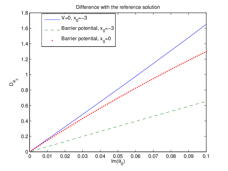
In the three tests described above, although some oscillations occur when crossing the interfaces x=−1x=-1 and x=1x=1, the quantitative comparison gives also good results. In particular, we represented in Figure 4 the variation with respect to Imθ0\mathop{\mathrm{Im}}~\theta_{0} of the maximum in time of the L2L^{2} relative difference:

Dθ0=max1≤n≤N⁡100​‖uθ0n−un‖‖uI‖,D_{\theta_{0}}=\max_{1\leq n\leq N}100\frac{\|u_{\theta_{0}}^{n}-u^{n}\|}{\|u_{I}\|}\,, (2.21)

where N=400N=400 is the number of time iterations. It shows that, for every case, the difference tends to 00 when Imθ0\mathop{\mathrm{Im}}~\theta_{0} tends to 00. Moreover, the graphic of Dθ0D_{\theta_{0}} is a line which validates the result (2.14). We note also that the difference in the case of a barrier potential is smaller then in the case V=0V=0. This may be due to the fact that the error coming from the interface conditions is compensated by the exponential decay imposed by the barrier. Then, in the case of a barrier potential, we note that the difference is more important when the initial condition is supported in (−1,1)(-1,1). It can be explained by the fact that the solution crosses the two interfaces, at x=−1x=-1 and x=1x=1, whereas, when the solution comes from the left, only the interaction with the first interface x=−1x=-1 is relevant, which is also a consequence of the exponential decay in the barrier.
Refer to caption
Figure 4: Variation with respect to Imθ0\mathop{\mathrm{Im}}~\theta_{0} of the difference Dθ0D_{\theta_{0}}, defined in (2.21), in the case V=0V=0 with x0=−3x_{0}=-3, and in the case of a barrier potential with x0=−3x_{0}=-3 and x0=0x_{0}=0

3 Exterior complex scaling and local perturbations

Spectral deformations of Schrödinger operators arising from complex dilations form a standard tool to study resonances. This technique – originally developed by J.M. Combes and coauthors in [3][10] for the homogeneous scaling in L2​(ℝn)L^{2}(\mathbb{R}^{n}): Uθ​ψ​(x)=en​θ2​ψ​(eθ​x)U_{\theta}\psi(x)=e^{\frac{n\theta}{2}}\psi(e^{\theta}x) – allows to relate the resonances of the Hamiltonian H=−Δ+𝒱H=-\Delta+\mathcal{V} with the spectral points of a non self-adjoint operator H⁡(θ)=Uθ​H​Uθ−1H(\theta)=U_{\theta}HU_{\theta}^{-1} with θ∈ℂ\theta\in\mathbb{C}. If the potential 𝒱\mathcal{V} is dilation analytic in the strip {θ∈ℂ||Imθ|<α}\left\{\theta\in\mathbb{C\,}\left|\,\left|\operatorname{Im}\theta\right|<\alpha\right.\right\}, the poles of the meromorphic continuation of the resolvent (H−z)−1\left(H-z\right)^{-1} in the second Riemann sheet are identified with the eigenvalues of H⁡(θ)H(\theta) placed in the cone spanned by the positive real axis and the rotated half axis e−2​i​Im⁡θ​ℝ+e^{-2i\operatorname{Im}\theta}\mathbb{R}_{+}. We refer the reader to [23] for a summary and we recall that many variations on this approach have been developed since, see [31][30][40] and [29] for a short comparison of these methods. In particular for potentials which can be complex deformed only outside a compact region, the exterior complex scaling technique appeared first in [54] in the singular version that we reconsider here. Meanwhile regular versions have been used in [31] and extended with the so called “black box” formalism in [56].

In this section, we consider a particular class of exterior scaling maps, UθU_{\theta}, acting outside a compact set in 1D and introducing sharp singularities in the domain of the corresponding deformed Hamiltonians. Let us introduce the one-parameter family of exterior dilations

x⟶{e−θ​(x−b)+b,x>bx,x∈(a,b)e−θ​(x−a)+a,x<a.x\longrightarrow\left\{\begin{array}[c]{ll}\vskip 3.0pt plus 1.0pt minus 1.0pte^{-\theta}(x-b)+b,&x>b\\ \vskip 3.0pt plus 1.0pt minus 1.0ptx,&x\in(a,b)\\ e^{-\theta}(x-a)+a,&x<a\,.\end{array}\right. (3.1)

For real values of the parameter θ\theta, the related unitary transformation in L2​(ℝ)L^{2}(\mathbb{R}) is

Uθ​ψ​(x)={eθ2​ψ​(eθ​(x−b)+b),x>bψ⁡(x),x∈(a,b)eθ2​ψ​(eθ​(x−a)+a),x<a.U_{\theta}\psi(x)=\left\{\begin{array}[c]{ll}e^{\frac{\theta}{2}}\psi(\vskip 3.0pt plus 1.0pt minus 1.0pte^{\theta}(x-b)+b),&x>b\\ \vskip 3.0pt plus 1.0pt minus 1.0pt\psi(x),&x\in(a,b)\\ e^{\frac{\theta}{2}}\psi(\vskip 3.0pt plus 1.0pt minus 1.0pte^{\theta}(x-a)+a),&x<a\,.\end{array}\right. (3.2)

Local perturbations of Hθ0,0h​(0)H_{\theta_{0},0}^{h}(0) are defined by

Hθ0,𝒱h​(0)=Hθ0,0h​(0)+𝒱,H_{\theta_{0},\mathcal{V}}^{h}(0)=H_{\theta_{0},0}^{h}(0)+\mathcal{V}\,, (3.3)

with supp​𝒱⊂[a,b]\mathrm{supp}\,\mathcal{V}\subset[a,b]. In what follows we will assume

𝒱=𝒱1+𝒱2,𝒱1∈L∞​((a,b)),𝒱2∈ℳb​(U)with ​U⊂⊂(a,b).\mathcal{V}=\mathcal{V}_{1}+\mathcal{V}_{2},\quad\mathcal{V}_{1}\in L^{\infty}((a,b)),\quad\mathcal{V}_{2}\in\mathcal{M}_{b}(U)\qquad\text{with }U\subset\subset(a,b)\,. (3.4)

Under these assumptions,

D(Hθ0,𝒱h(0))={u∈H2(ℝ\{a,b,U})|(1−χ)u∈D(Hθ0,0h(0)),−h2u′′+𝒱2u∈L2(U)},D(H_{\theta_{0},\mathcal{V}}^{h}(0))=\left\{u\in H^{2}(\mathbb{R}\backslash\left\{a,b,U\right\})\left|\ (1-\chi)u\in D(H_{\theta_{0},0}^{h}(0)),\,-h^{2}u^{\prime\prime}+\mathcal{V}_{2}u\in L^{2}(U)\right.\right\}\,,

where χ∈C0∞​((a,b))\chi\in C^{\infty}_{0}((a,b)) and χ⁡(x)=1\chi(x)=1 for x∈Ux\in U.
In particular, since 𝒱2\mathcal{V}_{2} is a bounded measure, the domain D⁡(Hθ0,𝒱h​(0))D(H_{\theta_{0},\mathcal{V}}^{h}(0)) is contained in H1​(ℝ\{a,b})H^{1}(\mathbb{R}\backslash\left\{a,b\right\}). The conjugated operator

Hθ0,𝒱h​(θ)=Uθ​Hθ0,𝒱h​(0)​Uθ−1H_{\theta_{0},\mathcal{V}}^{h}(\theta)=U_{\theta}H_{\theta_{0},\mathcal{V}}^{h}(0)U_{\theta}^{-1} (3.5)

is defined on D(Hθ0,𝒱h(θ))={u∈L2(ℝ)|Uθ−1u∈D(Hθ0,𝒱h(0))}D(H_{\theta_{0},\mathcal{V}}^{h}(\theta))=\left\{u\in L^{2}(\mathbb{R})\left|\,U_{\theta}^{-1}u\in D(H_{\theta_{0},\mathcal{V}}^{h}(0))\right.\right\}. The constraint Uθ−1​u∈D⁡(Hθ0,𝒱h​(0))U_{\theta}^{-1}u\in D(H_{\theta_{0},\mathcal{V}}^{h}(0)) compels the boundary conditions

[e−12​(θ0+θ)​u​(b+)=u⁡(b−);e−32​(θ0+θ)​u′​(b+)=u′​(b−)e−12​(θ0+θ)u(a−)=u(a+);e−32​(θ0+θ)u′(a−)=u′(a+),\left[\begin{array}[c]{l}e^{-\frac{1}{2}\left(\theta_{0}+\theta\right)}u(b^{+})=u(b^{-});\quad\vskip 6.0pt plus 2.0pt minus 2.0pte^{-\frac{3}{2}\left(\theta_{0}+\theta\right)}u^{\prime}(b^{+})=u^{\prime}(b^{-})\\ e^{-\frac{1}{2}\left(\theta_{0}+\theta\right)}u(a^{-})=u(a^{+});\quad e^{-\frac{3}{2}\left(\theta_{0}+\theta\right)}u^{\prime}(a^{-})=u^{\prime}(a^{+})\,,\end{array}\right. (3.6)

to hold for any u∈D⁡(Hθ0,𝒱h​(θ))u\in D(H_{\theta_{0},\mathcal{V}}^{h}(\theta)). Thus one has

D(Hθ0,𝒱h(θ))={u∈H2(ℝ\{a,b,U})∩H1(ℝ\{a,b})|(3.6),−h2u′′+𝒱2u∈L2(U)}.D(H_{\theta_{0},\mathcal{V}}^{h}(\theta))=\left\{u\in H^{2}(\mathbb{R}\backslash\left\{a,b,U\right\})\cap H^{1}(\mathbb{R}\backslash\left\{a,b\right\})\left|\ \left(\ref{BC_1}\right),\ -h^{2}u^{\prime\prime}+\mathcal{V}_{2}u\in L^{2}(U)\right.\right\}. (3.7)

The action of Hθ0,𝒱h​(θ)H_{\theta_{0},\mathcal{V}}^{h}(\theta) is

Hθ0,𝒱h(θ)u=[−h2η(x)∂x2+𝒱]u,η(x)=e−2​θ​ 1ℝ∖(a,b)​(x).H_{\theta_{0},\mathcal{V}}^{h}(\theta)u=\left[-h^{2}\eta(x)\partial_{x}^{2}+\mathcal{V}\right]\,u,\qquad\eta(x)=e^{-2\theta\,1_{\mathbb{R}\setminus(a,b)}(x)}\,. (3.8)

It is worthwhile to notice that this definition can be extended to complex values of θ\theta. For θ∈ℂ\theta\in\mathbb{C}, the Hamiltonian Hθ0,𝒱h​(θ)H_{\theta_{0},\mathcal{V}}^{h}(\theta) identifies with a restriction of the operator Q⁡(θ)Q(\theta)

{D(Q(θ))={u∈H2(ℝ\{a,b,U})∩H1(ℝ\{a,b})|−h2u′′+𝒱2u∈L2(U)},Q(θ)u=[−h2η(x)∂x2+𝒱]u.\left\{\begin{array}[c]{l}\vskip 6.0pt plus 2.0pt minus 2.0ptD(Q(\theta))=\left\{u\in H^{2}(\mathbb{R}\backslash\left\{a,b,U\right\})\cap H^{1}(\mathbb{R}\backslash\left\{a,b\right\})\left|\ -h^{2}u^{\prime\prime}+\mathcal{V}_{2}u\in L^{2}(U)\right.\right\}\,,\\ Q(\theta)u=\left[-h^{2}\eta(x)\partial_{x}^{2}+\mathcal{V}\right]\,u\,.\end{array}\right. (3.9)

For particular choices of θ0\theta_{0} and θ\theta, the quantum evolution generated by the deformed model Hθ0,𝒱h​(θ)H_{\theta_{0},\mathcal{V}}^{h}(\theta) is described by contraction maps. To fix this point, let us consider the terms
Re⁡⟨u,i​Hθ0,𝒱h​(θ)​u⟩L2​(ℝ)\operatorname{Re}\left\langle u,iH_{\theta_{0},\mathcal{V}}^{h}(\theta)u\right\rangle_{L^{2}(\mathbb{R})}; for u∈D⁡(Hθ0,𝒱h​(θ))u\in D(H_{\theta_{0},\mathcal{V}}^{h}(\theta)), an explicit calculation gives

Re⁡⟨u,i​Hθ0,𝒱h​(θ)​u⟩L2​(ℝ)\displaystyle\operatorname{Re}\left\langle u,iH_{\theta_{0},\mathcal{V}}^{h}(\theta)u\right\rangle_{L^{2}(\mathbb{R})} =Re⁡{−i​h2​(u¯​(a−)​u′​(a−)−u¯​(b+)​u′​(b+))​(e−2​θ−e−12​(θ¯+θ¯0)​e−32​(θ+θ0))}\displaystyle=\operatorname{Re}\left\{-ih^{2}\left(\bar{u}(a^{-})u^{\prime}(a^{-})-\bar{u}(b^{+})u^{\prime}(b^{+})\right)\,\left(e^{-2\theta}-e^{-\frac{1}{2}\left(\bar{\theta}+\bar{\theta}_{0}\right)}e^{-\frac{3}{2}\left(\theta+\theta_{0}\right)}\right)\right\}
+h2e−2​Re⁡θsin(2Imθ)∫ℝ\(a,b)|u′|2dx.\displaystyle+h^{2}e^{-2\operatorname{Re}\theta}\sin\left(2\operatorname{Im}\theta\right)\int_{\mathbb{R}\backslash\left(a,b\right)}\left|u^{\prime}\right|^{2}dx. (3.10)

For θ=θ0=i​τ\theta=\theta_{0}=i\tau, with τ∈(0,π2)\tau\in\left(0,\frac{\pi}{2}\right), the boundary terms disappear, and the r.h.s. of (3.10) is positive

Re⁡⟨u,i​Hi​τ,𝒱h​(i​τ)​u⟩L2​(ℝ)=h2​sin⁡(2​τ)​∫ℝ\(a,b)|u′|2​𝑑x≥0.\operatorname{Re}\left\langle u,iH_{i\tau,\mathcal{V}}^{h}(i\tau)u\right\rangle_{L^{2}(\mathbb{R})}=h^{2}\sin\left(2\tau\right)\int_{\mathbb{R}\backslash\left(a,b\right)}\left|u^{\prime}\right|^{2}dx\geq 0. (3.11)
Lemma 3.1.

For τ∈(0,π2)\tau\in\left(0,\frac{\pi}{2}\right), the operator i​Hi​τ,𝒱h​(i​τ)iH_{i\tau,\mathcal{V}}^{h}(i\tau) is the generator of a contraction semigroup.

Proof: As a consequence of (3.11), i​Hi​τ,𝒱h​(i​τ)iH_{i\tau,\mathcal{V}}^{h}(i\tau) is accretive. Moreover, the propriety σe​s​s​(Hi​τ,𝒱h​(i​τ))=e−2​i​τ​ℝ+\sigma_{ess}\left(H_{i\tau,\mathcal{V}}^{h}(i\tau)\right)=e^{-2i\tau}\mathbb{R}_{+} in Corollary 3.4 below, implies i​λ0∈ρ⁡(Hi​τ,𝒱h​(i​τ))i\lambda_{0}\in\rho(H_{i\tau,\mathcal{V}}^{h}(i\tau)) for some λ0>0\lambda_{0}>0 and (i​Hi​τ,𝒱h​(i​τ)+λ0)\left(iH_{i\tau,\mathcal{V}}^{h}(i\tau)+\lambda_{0}\right) is surjective. Then, a standard characterization of semigroup generators ([51], Theorem X.48) leads to the result. ∎

3.1 Krein formula and analyticity of the resolvent

In order to get an expression of the adjoint operator of Hθ0,𝒱h​(θ)H_{\theta_{0},\mathcal{V}}^{h}(\theta), we introduce the following operator with two-parameters boundary conditions

D(𝒬θ1,θ2(θ))={u∈D(Q(θ))|[e−12​(θ1+θ)​u​(b+)=u⁡(b−);e−12​(θ2+3​θ)​u′​(b+)=u′​(b−)e−12​(θ1+θ)​u​(a−)=u⁡(a+);e−12​(θ2+3​θ)​u′​(a−)=u′​(a+)},D(\mathcal{Q}_{\theta_{1},\theta_{2}}(\theta))=\left\{u\in D(Q(\theta))\left|\ \left[\begin{array}[c]{l}e^{-\frac{1}{2}\left(\theta_{1}+\theta\right)}u(b^{+})=u(b^{-});\quad\vskip 6.0pt plus 2.0pt minus 2.0pte^{-\frac{1}{2}\left(\theta_{2}+3\theta\right)}u^{\prime}(b^{+})=u^{\prime}(b^{-})\\ e^{-\frac{1}{2}\left(\theta_{1}+\theta\right)}u(a^{-})=u(a^{+});\quad e^{-\frac{1}{2}\left(\theta_{2}+3\theta\right)}u^{\prime}(a^{-})=u^{\prime}(a^{+})\end{array}\right.\right.\right\}\,, (3.12)
𝒬θ1,θ2(θ)u=[−h2η(x)∂x2+𝒱]u,η(x)=e−2​θ​ 1ℝ∖(a,b)​(x),\mathcal{Q}_{\theta_{1},\theta_{2}}(\theta)u=\left[-h^{2}\eta(x)\partial_{x}^{2}+\mathcal{V}\right]u,\qquad\eta(x)=e^{-2\theta\,1_{\mathbb{R}\setminus(a,b)}(x)}\,, (3.13)

where Q⁡(θ)Q(\theta) is defined in (3.9). Indeed, by direct computation
i) 𝒬θ1,θ2​(θ)\mathcal{Q}_{\theta_{1},\theta_{2}}(\theta) identifies with the original model Hθ0,𝒱h​(θ)H_{\theta_{0},\mathcal{V}}^{h}(\theta) for the choice of parameters: θ1=θ0\theta_{1}=\theta_{0} and θ2=3​θ0\theta_{2}=3\theta_{0}

Hθ0,𝒱h​(θ)=𝒬θ0,3​θ0​(θ),H_{\theta_{0},\mathcal{V}}^{h}(\theta)=\mathcal{Q}_{\theta_{0},3\theta_{0}}(\theta), (3.14)

ii) the adjoint operator (𝒬θ1,θ2​(θ))∗\left(\mathcal{Q}_{\theta_{1},\theta_{2}}(\theta)\right)^{\ast} is given by

(𝒬θ1,θ2​(θ))∗=𝒬−θ¯2,−θ¯1​(θ¯).\left(\mathcal{Q}_{\theta_{1},\theta_{2}}(\theta)\right)^{\ast}=\mathcal{Q}_{-\bar{\theta}_{2},-\bar{\theta}_{1}}(\bar{\theta}). (3.15)

Like Hθ0,𝒱h​(θ)H_{\theta_{0},\mathcal{V}}^{h}(\theta), the Hamiltonian 𝒬θ1,θ2​(θ)\mathcal{Q}_{\theta_{1},\theta_{2}}(\theta) is a restriction of the operator Q⁡(θ)Q(\theta). In this context, we fix a boundary value triple {Γj=1,2θ,ℂ4}\left\{\Gamma_{j=1,2}^{\theta},\mathbb{C}^{4}\right\} with Γjθ:D⁡(Q⁡(θ))→ℂ4\Gamma_{j}^{\theta}:D(Q(\theta))\rightarrow\mathbb{C}^{4}

Γ1θ​ψ=h2​(−e−32​θ​ψ′​(b+)−ψ⁡(b−)ψ⁡(a+)e−32​θ​ψ′​(a−));Γ2θ​ψ=(e−θ2​ψ​(b+)ψ′​(b−)ψ′​(a+)e−θ2​ψ​(a−)),\Gamma_{1}^{\theta}\psi=h^{2}\left(\begin{array}[c]{c}-e^{-\frac{3}{2}\theta}\psi^{\prime}(b^{+})\\ -\psi(b^{-})\\ \psi(a^{+})\\ e^{-\frac{3}{2}\theta}\psi^{\prime}(a^{-})\end{array}\right);\qquad\Gamma_{2}^{\theta}\psi=\left(\begin{array}[c]{c}e^{-\frac{\theta}{2}}\psi(b^{+})\\ \psi^{\prime}(b^{-})\\ \psi^{\prime}(a^{+})\\ e^{-\frac{\theta}{2}}\psi(a^{-})\end{array}\right)\,, (3.16)

and (Γ1θ,Γ2θ):D⁡(Q​(θ)∗)→ℂ4×ℂ4\left(\Gamma_{1}^{\theta},\Gamma_{2}^{\theta}\right):D(Q(\theta)^{\ast})\rightarrow\mathbb{C}^{4}\times\mathbb{C}^{4} surjective. For all ψ,φ∈D⁡(Q⁡(θ))\psi,\varphi\in D(Q(\theta)), these maps satisfy the relation

⟨ψ,Q⁡(θ)​φ⟩L2​(ℝ)−⟨Q⁡(θ¯)​ψ,φ⟩L2​(ℝ)=⟨Γ1θ¯​ψ,Γ2θ​φ⟩ℂ4−⟨Γ2θ¯​ψ,Γ1θ​φ⟩ℂ4\left\langle\psi,Q(\theta)\varphi\right\rangle_{L^{2}(\mathbb{R})}-\left\langle Q(\bar{\theta})\psi,\varphi\right\rangle_{L^{2}(\mathbb{R})}=\left\langle\Gamma_{1}^{\bar{\theta}}\psi,\Gamma_{2}^{\theta}\varphi\right\rangle_{\mathbb{C}^{4}}-\left\langle\Gamma_{2}^{\bar{\theta}}\psi,\Gamma_{1}^{\theta}\varphi\right\rangle_{\mathbb{C}^{4}} (3.17)

(for the definition of boundary triples and the construction of point interaction potentials in the self adjoint case see [47] and [4]). Let Λ,B∈ℂ4,4\Lambda,B\in\mathbb{C}^{4,4} be defined as

Λ⁡(θ1,θ2)=1h2​(a⁡(θ1,θ2)−a⁡(−θ2,−θ1)),B=(bb),\Lambda(\theta_{1},\theta_{2})=\frac{1}{h^{2}}\begin{pmatrix}a(\theta_{1},\theta_{2})&\\ &-a(-\theta_{2},-\theta_{1})\end{pmatrix},\qquad B=\begin{pmatrix}b&\\ &b\end{pmatrix}, (3.18)
a⁡(θ1,θ2)=(−e−θ2200−eθ12),b=(0110),a(\theta_{1},\theta_{2})=\begin{pmatrix}-e^{-\frac{\theta_{2}}{2}}&0\\ 0&-e^{\frac{\theta_{1}}{2}}\end{pmatrix},\quad\quad b=\begin{pmatrix}0&1\\ 1&0\end{pmatrix}, (3.19)

the boundary conditions in (3.12) are equivalent to

Λ​Γ1θ​ψ=B​Γ2θ​ψ.\Lambda\Gamma_{1}^{\theta}\psi=B\Gamma_{2}^{\theta}\psi\,. (3.20)

Let HN​D,𝒱h​(θ)H_{ND,\mathcal{V}}^{h}(\theta) denote the restriction of Q⁡(θ)Q(\theta) corresponding to the boundary conditions: Γ1θ​ψ=0\Gamma_{1}^{\theta}\psi=0; this operator is explicitly given by

HN​D,𝒱h​(θ)=−h2​e−2​θ​Δ(−∞,a)N⊕[−h2​Δ(a,b)D+𝒱]⊕−h2​e−2​θ​Δ(b,+∞)N.H_{ND,\mathcal{V}}^{h}(\theta)=-h^{2}e^{-2\theta}\Delta_{(-\infty,a)}^{N}\oplus\left[-h^{2}\Delta_{(a,b)}^{D}+\mathcal{V}\right]\oplus-h^{2}e^{-2\theta}\Delta_{(b,+\infty)}^{N}. (3.21)

Its spectrum is characterized as follows

σ⁡(HN​D,𝒱h​(θ))=e−2​θ​ℝ+∪σ⁡(−h2​Δ(a,b)D+𝒱).\sigma\left(H_{ND,\mathcal{V}}^{h}(\theta)\right)=e^{-2\theta}\mathbb{R}_{+}\cup\sigma\left(-h^{2}\Delta_{(a,b)}^{D}+\mathcal{V}\right)\,. (3.22)

It is possible to write (𝒬θ1,θ2​(θ)−z)−1\left(\mathcal{Q}_{\theta_{1},\theta_{2}}(\theta)-z\right)^{-1} as the sum of (HN​D,𝒱h​(θ)−z)−1\left(H_{ND,\mathcal{V}}^{h}(\theta)-z\right)^{-1} plus finite rank terms. Such a representation will be further used to develop the spectral analysis of Hθ0,𝒱h​(θ)H_{\theta_{0},\mathcal{V}}^{h}(\theta) where our Krein-like formula will allow explicit resolvent estimates near the resonances. The space 𝒩z,θ=Ker⁡(Q⁡(θ)−z)\mathcal{N}_{z,\theta}=\mathrm{Ker}(Q(\theta)-z) is generated by the linear closure of the system {ui,z}i=14\left\{u_{i,z}\right\}_{i=1}^{4} where ui,zu_{i,z} are the independent solutions to (Q⁡(θ)−z)​u=0(Q(\theta)-z)u=0. The exterior solutions to this problem, ui,zu_{i,z}, i=1,4i=1,4, are explicitly given by

u1,z​(x)=1(b,+∞)​ei​z​e2​θh​(x−b),u4,z​(x)=1(−∞,a)​e−i​z​e2​θh​(x−a),u_{1,z}(x)=1_{\left(b,+\infty\right)}e^{i\frac{\sqrt{ze^{2\theta}}}{h}(x-b)},\quad u_{4,z}(x)=1_{\left(-\infty,a\right)}e^{-i\frac{\sqrt{ze^{2\theta}}}{h}(x-a)}, (3.23)

where the square root branch cut is fixed with Im⁡⋅>0\operatorname{Im}\sqrt{\cdot}>0. This assumption implies Imz​e2​θ>0\mathop{\mathrm{Im}}~\sqrt{ze^{2\theta}}~>~0 for all z∈ℂ\e−2​i​Im⁡θ​ℝ+z\in\mathbb{C}\backslash e^{-2i\operatorname{Im}\theta}\mathbb{R}_{+}. The interior solutions, ui,zu_{i,z}, i=2,3i=2,3, can be defined through the following boundary value problems

{[−h2∂x2+𝒱−z]u2,z=0,in (a,b),u2,z(a)=0,u2,z(b)=1,{[−h2∂x2+𝒱−z]u3,z=0,in (a,b),u3,z(a)=1,u3,z(b)=0,\left\{\begin{array}[c]{l}\vskip 6.0pt plus 2.0pt minus 2.0pt\left[-h^{2}\partial_{x}^{2}+\mathcal{V}-z\right]\,u_{2,z}=0,\qquad\text{in }\left(a,b\right)\,,\\ u_{2,z}(a)=0,\qquad u_{2,z}(b)=1\,,\end{array}\right.\quad\left\{\begin{array}[c]{l}\vskip 6.0pt plus 2.0pt minus 2.0pt\left[-h^{2}\partial_{x}^{2}+\mathcal{V}-z\right]\,u_{3,z}=0,\qquad\text{in }\left(a,b\right)\,,\\ u_{3,z}(a)=1,\qquad u_{3,z}(b)=0\,,\end{array}\right. (3.24)

with z∈ℂ\σp​(HN​D,𝒱h​(θ))z\in\mathbb{C}\backslash\sigma_{p}(H_{ND,\mathcal{V}}^{h}(\theta)). Owing to the property of the interior Dirichlet realization in (a,b)(a,b), the solutions ui,z|(a,b)u_{i,z}\big|_{(a,b)} are unique and locally H2H^{2} near the boundary. We consider the maps: γ⁡(⋅,z,θ)=(Γ1θ|𝒩z,θ)−1\gamma(\cdot,z,\theta)=\left(\left.\Gamma_{1}^{\theta}\right|_{\mathcal{N}_{z,\theta}}\right)^{-1}, with Γ1θ|𝒩z,θ\left.\Gamma_{1}^{\theta}\right|_{\mathcal{N}_{z,\theta}} denoting the restriction of Γ1θ\Gamma_{1}^{\theta} onto 𝒩z,θ\mathcal{N}_{z,\theta}, and q⁡(z,θ,𝒱)=Γ2θ​γ​(⋅,z,θ)q(z,\theta,\mathcal{V})=\Gamma_{2}^{\theta}\gamma(\cdot,z,\theta). These form holomorphic families of linear operators for zz in a cut plane ℂ\e−2​i​Im⁡θ​ℝ+\mathbb{C}\backslash e^{-2i\operatorname{Im}\theta}\mathbb{R}_{+}. Their matrix form w.r.t. the standard basis {e¯j}j=14\left\{\underline{e}_{j}\right\}_{j=1}^{4} of ℂ4\mathbb{C}^{4} and the system {ui,z}i=14\left\{u_{i,z}\right\}_{i=1}^{4} is: γi​j​(z,θ)=ci​(z,θ)​δi​j\gamma_{ij}(z,\theta)=c_{i}(z,\theta)\delta_{ij} with

c1​(z,θ)=i​e3​θ2h​z​e2​θ,c2=−1h2,c3=1h2,c4​(z,θ)=i​e3​θ2h​z​e2​θ,c_{1}(z,\theta)=\frac{ie^{\frac{3\theta}{2}}}{h\sqrt{ze^{2\theta}}},\ c_{2}=-\frac{1}{h^{2}},\ c_{3}=\frac{1}{h^{2}},\ c_{4}(z,\theta)=\frac{ie^{\frac{3\theta}{2}}}{h\sqrt{ze^{2\theta}}}\,, (3.25)

and

q⁡(z,θ,𝒱)=1h2​(i​h​eθz​e2​θ−u2,z′​(b)u3,z′​(b)−u2,z′​(a)u3,z′​(a)i​h​eθz​e2​θ).q(z,\theta,\mathcal{V})=\frac{1}{h^{2}}\begin{pmatrix}\frac{ihe^{\theta}}{\sqrt{ze^{2\theta}}}&&&\\ &-u_{2,z}^{\prime}(b)&u_{3,z}^{\prime}(b)&\\ &-u_{2,z}^{\prime}(a)&u_{3,z}^{\prime}(a)&\\ &&&\frac{ihe^{\theta}}{\sqrt{ze^{2\theta}}}\end{pmatrix}. (3.26)
Lemma 3.2.

Let φ∈L2​(ℝ)\varphi\in L^{2}(\mathbb{R}) and j=1,…,4j=1,...,4; the relation

[Γ2θ​(HN​D,𝒱h​(θ)−z)−1​φ]j=⟨γ⁡(e¯j,z¯,θ¯),φ⟩L2​(ℝ)\left[\Gamma_{2}^{\theta}\left(H_{ND,\mathcal{V}}^{h}(\theta)-z\right)^{-1}\varphi\right]_{j}=\left\langle\gamma(\underline{e}_{j},\bar{z},\bar{\theta}),\varphi\right\rangle_{L^{2}(\mathbb{R})} (3.27)

holds with θ∈ℂ\theta\in\mathbb{C} and z∈ρ⁡(HN​D,𝒱h​(θ))z\in\rho\,\left(H_{ND,\mathcal{V}}^{h}(\theta)\right).

Proof: Let: f=(HN​D,𝒱h​(θ)−z)−1​φf=\left(H_{ND,\mathcal{V}}^{h}(\theta)-z\right)^{-1}\varphi. This function is in D⁡(HN​D,𝒱h​(θ))D(H_{ND,\mathcal{V}}^{h}(\theta)) so that:
Q⁡(θ)​f=HN​D,𝒱h​(θ)​fQ(\theta)f=H_{ND,\mathcal{V}}^{h}(\theta)f and Γ1θ​f=0\Gamma_{1}^{\theta}f=0. The l.h.s of (3.27) writes as

[Γ2θ​(HN​D,𝒱h​(θ)−z)−1​φ]j=⟨e¯j,Γ2θ​f⟩ℂ4.\left[\Gamma_{2}^{\theta}\left(H_{ND,\mathcal{V}}^{h}(\theta)-z\right)^{-1}\varphi\right]_{j}=\left\langle\underline{e}_{j},\,\Gamma_{2}^{\theta}f\right\rangle_{\mathbb{C}^{4}}.

Since e¯j=Γ1θ¯​γ​(e¯j,z¯,θ¯)\underline{e}_{j}=\Gamma_{1}^{\bar{\theta}}\gamma(\underline{e}_{j},\bar{z},\bar{\theta}), we have

[Γ2θ​(HN​D,𝒱h​(θ)−z)−1​φ]j\displaystyle\left[\Gamma_{2}^{\theta}\left(H_{ND,\mathcal{V}}^{h}(\theta)-z\right)^{-1}\varphi\right]_{j} =⟨Γ1θ¯​γ​(e¯j,z¯,θ¯),Γ2θ​f⟩ℂ4−⟨Γ2θ¯​γ​(e¯j,z¯,θ¯),Γ1θ​f⟩ℂ4\displaystyle=\left\langle\Gamma_{1}^{\bar{\theta}}\gamma(\underline{e}_{j},\bar{z},\bar{\theta}),\,\Gamma_{2}^{\theta}f\right\rangle_{\mathbb{C}^{4}}-\left\langle\Gamma_{2}^{\bar{\theta}}\gamma(\underline{e}_{j},\bar{z},\bar{\theta}),\,\Gamma_{1}^{\theta}f\right\rangle_{\mathbb{C}^{4}}
=⟨γ⁡(e¯j,z¯,θ¯),Q⁡(θ)​f⟩L2​(ℝ)−⟨Q⁡(θ¯)​γ​(e¯j,z¯,θ¯),f⟩L2​(ℝ).\displaystyle=\left\langle\gamma(\underline{e}_{j},\bar{z},\bar{\theta}),\,Q(\theta)f\right\rangle_{L^{2}(\mathbb{R})}-\left\langle Q(\bar{\theta})\gamma(\underline{e}_{j},\bar{z},\bar{\theta}),\,f\right\rangle_{L^{2}(\mathbb{R})}.

By definition, γ⁡(e¯j,z¯,θ¯)∈𝒩z¯,θ¯\gamma(\underline{e}_{j},\bar{z},\bar{\theta})\in\mathcal{N}_{\bar{z},\bar{\theta}} and the r.h.s. writes as

⟨γ⁡(e¯j,z¯,θ¯),Q⁡(θ)​f⟩L2​(ℝ)−⟨Q⁡(θ¯)​γ​(e¯j,z¯,θ¯),f⟩L2​(ℝ)\displaystyle\left\langle\gamma(\underline{e}_{j},\bar{z},\bar{\theta}),\,Q(\theta)f\right\rangle_{L^{2}(\mathbb{R})}-\left\langle Q(\bar{\theta})\gamma(\underline{e}_{j},\bar{z},\bar{\theta}),\,f\right\rangle_{L^{2}(\mathbb{R})} =⟨γ⁡(e¯j,z¯,θ¯),(HN​D,𝒱h​(θ)−z)​f⟩L2​(ℝ)\displaystyle=\left\langle\gamma(\underline{e}_{j},\bar{z},\bar{\theta}),\,\,\left(H_{ND,\mathcal{V}}^{h}(\theta)-z\right)f\right\rangle_{L^{2}(\mathbb{R})}
=⟨γ⁡(e¯j,z¯,θ¯),φ⟩L2​(ℝ).\displaystyle=\left\langle\gamma(\underline{e}_{j},\bar{z},\bar{\theta}),\,\varphi\right\rangle_{L^{2}(\mathbb{R})}.

∎

Proposition 3.3.

The resolvent (𝒬θ1,θ2​(θ)−z)−1\left(\mathcal{Q}_{\theta_{1},\theta_{2}}(\theta)-z\right)^{-1} allows the representation

(𝒬θ1,θ2​(θ)−z)−1\displaystyle\left(\mathcal{Q}_{\theta_{1},\theta_{2}}(\theta)-z\right)^{-1} =(HN​D,𝒱h​(θ)−z)−1\displaystyle=\left(H_{ND,\mathcal{V}}^{h}(\theta)-z\right)^{-1}
−∑i,j=14[(Bq(z,θ,𝒱)−Λ)−1B]i​j⟨γ(e¯j,z¯,θ¯),⋅⟩L2​(ℝ)γ(e¯i,z,θ),\displaystyle-\sum_{i,j=1}^{4}\left[\left(Bq(z,\theta,\mathcal{V})-\Lambda\right)^{-1}B\right]_{ij}\left\langle\gamma(\underline{e}_{j},\bar{z},\bar{\theta}),\cdot\right\rangle_{L^{2}(\mathbb{R})}\gamma(\underline{e}_{i},z,\theta), (3.28)

and one has: σe​s​s​(𝒬θ1,θ2​(θ))=σe​s​s​(HN​D,𝒱h​(θ))=e−2​θ​ℝ+\sigma_{ess}(\mathcal{Q}_{\theta_{1},\theta_{2}}(\theta))=\sigma_{ess}(H_{ND,\mathcal{V}}^{h}(\theta))=e^{-2\theta}\mathbb{R}_{\mathbb{+}}.

Proof: Let us consider the r.h.s. of this formula: the operator (HN​D,𝒱h​(θ)−z)−1\left(H_{ND,\mathcal{V}}^{h}(\theta)-z\right)^{-1} is well defined for z∈ℂ\σ⁡(HN​D,𝒱h​(θ))z\in\mathbb{C}\backslash\sigma(H_{ND,\mathcal{V}}^{h}(\theta)). The vectors γ⁡(e¯i,z,θ)\gamma(\underline{e}_{i},z,\theta), i=1,…,4i=1,...,4, are given by (3.23), (3.24), (3.25), while the boundary values of ui,z′u_{i,z}^{\prime} – appearing in the definition of the matrix (3.26) – are well defined whenever z∈ℂ\σp​(HN​D,𝒱h​(θ))z\in\mathbb{C}\backslash\sigma_{p}(H_{ND,\mathcal{V}}^{h}(\theta)). Therefore, the r.h.s. of (3.28) makes sense for z∈ℂ\{σ⁡(HN​D,𝒱h​(θ))∪𝒯0}z\in\mathbb{C}\backslash\left\{\sigma(H_{ND,\mathcal{V}}^{h}(\theta))\cup\mathcal{T}_{0}\right\} where 𝒯0\mathcal{T}_{0} is the (at most) discrete set, described by the transcendental equation

det(B​q​(z,θ,𝒱)−Λ⁡(θ1,θ2))=0.\det\left(Bq(z,\theta,\mathcal{V})-\Lambda(\theta_{1},\theta_{2})\right)=0. (3.29)

It is worthwhile to notice that ℂ\{σ⁡(HN​D,𝒱h​(θ))∪𝒯0}\mathbb{C}\backslash\left\{\sigma(H_{ND,\mathcal{V}}^{h}(\theta))\cup\mathcal{T}_{0}\right\} is not empty. Let us introduce the map Rz​(φ)R_{z}(\varphi) defined for φ∈L2​(ℝ)\varphi\in L^{2}(\mathbb{R}) by

Rz​(φ)=ϕ−ψ,R_{z}(\varphi)=\phi-\psi,
ϕ=(HN​D,𝒱h​(θ)−z)−1​φ,\phi=\left(H_{ND,\mathcal{V}}^{h}(\theta)-z\right)^{-1}\varphi,
ψ=∑i,j=14[(B​q​(z,θ,𝒱)−Λ)−1​B]i​j​⟨γ⁡(e¯j,z¯,θ¯),φ⟩L2​(ℝ)​γ​(e¯i,z,θ),\psi=\sum_{i,j=1}^{4}\left[\left(Bq(z,\theta,\mathcal{V})-\Lambda\right)^{-1}B\right]_{ij}\left\langle\gamma(\underline{e}_{j},\bar{z},\bar{\theta}),\varphi\right\rangle_{L^{2}(\mathbb{R})}\gamma(\underline{e}_{i},z,\theta),

with q⁡(z,θ,𝒱)q(z,\theta,\mathcal{V}) given in (3.26) and z∈ρ⁡(HN​D,𝒱h​(θ))\𝒯0z\in\rho(H_{ND,\mathcal{V}}^{h}(\theta))\backslash\mathcal{T}_{0}. In what follows we show that:
Rz​(φ)=(𝒬θ1,θ2​(θ)−z)−1​φR_{z}(\varphi)~=~\left(\mathcal{Q}_{\theta_{1},\theta_{2}}(\theta)-z\right)^{-1}\varphi. Since HN​D,𝒱h​(θ)⊂Q⁡(θ)H_{ND,\mathcal{V}}^{h}(\theta)\subset Q(\theta) and γ⁡(e¯i,z,θ)∈Ker⁡(Q⁡(θ)−z)\gamma(\underline{e}_{i},z,\theta)\in\mathrm{Ker}(Q(\theta)-z), one has:

(HN​D,𝒱h​(θ)−z)−1​φ,γ⁡(e¯i,z,θ)∈D⁡(Q⁡(θ)).\left(H_{ND,\mathcal{V}}^{h}(\theta)-z\right)^{-1}\varphi,\,\gamma(\underline{e}_{i},z,\theta)\in D(Q(\theta))\,.

This implies Rz​(φ)∈D⁡(Q⁡(θ))R_{z}(\varphi)\in D(Q(\theta)). To simplify the presentation, we will temporarily use the notation q=q⁡(z,θ,𝒱)q=q(z,\theta,\mathcal{V}). Being ϕ∈D⁡(HN​D,𝒱h​(θ))\phi\in D(H_{ND,\mathcal{V}}^{h}(\theta)), we have: Γ1θ​ϕ=0\Gamma_{1}^{\theta}\phi=0 and the following relation holds

(B​q−Λ)​Γ1θ​(ϕ−ψ)=−(B​Γ2θ​γ​(⋅,z,θ)−Λ)​Γ1θ​ψ=(−B​Γ2θ+Λ​Γ1θ)​ψ,\left(Bq-\Lambda\right)\Gamma_{1}^{\theta}\left(\phi-\psi\right)=-\left(B\Gamma_{2}^{\theta}\gamma(\cdot,z,\theta)-\Lambda\right)\Gamma_{1}^{\theta}\psi=\left(-B\Gamma_{2}^{\theta}+\Lambda\Gamma_{1}^{\theta}\right)\psi, (3.30)

where ψ∈𝒩z,θ\psi\in\mathcal{N}_{z,\theta} and

γ⁡(⋅,z,θ)​Γ1θ|𝒩z,θ=1\gamma(\cdot,z,\theta)\Gamma_{1}^{\theta}|_{\mathcal{N}_{z,\theta}}=1

have been used. At the same time, the nn-th component of the vector at the l.h.s. can be expressed as

[(B​q−Λ)​Γ1θ​(ϕ−ψ)]n=[−(B​q−Λ)​Γ1θ​ψ]n=−∑i,j=14[(Bq−Λ)Γ1θγ(e¯i,z,θ)]n[(Bq−Λ)−1B]i​j⟨γ(e¯j,z¯,θ¯),φ⟩L2​(ℝ).\left[\vskip 3.0pt plus 1.0pt minus 1.0pt\left(Bq-\Lambda\right)\Gamma_{1}^{\theta}\left(\phi-\psi\right)\right]_{n}=\left[-\left(Bq-\Lambda\right)\Gamma_{1}^{\theta}\psi\right]_{n}\\ =-\sum_{i,j=1}^{4}\left[\left(Bq-\Lambda\right)\Gamma_{1}^{\theta}\gamma(\underline{e}_{i},z,\theta)\right]_{n}\,\left[\left(Bq-\Lambda\right)^{-1}B\right]_{ij}\left\langle\gamma(\underline{e}_{j},\bar{z},\bar{\theta}),\varphi\right\rangle_{L^{2}(\mathbb{R})}.

Recalling that Γ1θ​γ​(e¯i,z,θ)=ei\Gamma_{1}^{\theta}\gamma(\underline{e}_{i},z,\theta)=e_{i}, we get

[(B​q−Λ)​Γ1θ​(ϕ−ψ)]n=−∑i,j=14(Bq−Λ)n​i[(Bq−Λ)−1B]i​j⟨γ(e¯j,z¯,θ¯),φ⟩L2​(ℝ)=−∑j=14Bn​j⟨γ(e¯j,z¯,θ¯),φ⟩L2​(ℝ).\left[\vskip 3.0pt plus 1.0pt minus 1.0pt\left(Bq-\Lambda\right)\Gamma_{1}^{\theta}\left(\phi-\psi\right)\right]_{n}=\\ -\sum_{i,j=1}^{4}\left(Bq-\Lambda\right)_{ni}\,\left[\left(Bq-\Lambda\right)^{-1}B\right]_{ij}\left\langle\gamma(\underline{e}_{j},\bar{z},\bar{\theta}),\varphi\right\rangle_{L^{2}(\mathbb{R})}=-\sum_{j=1}^{4}B_{nj}\left\langle\gamma(\underline{e}_{j},\bar{z},\bar{\theta}),\varphi\right\rangle_{L^{2}(\mathbb{R})}.

Taking into account the result of the Lemma 3.2, this relation writes as

(B​q−Λ)​Γ1θ​(ϕ−ψ)=−B​Γ2θ​ϕ.\left(Bq-\Lambda\right)\Gamma_{1}^{\theta}\left(\phi-\psi\right)=-B\Gamma_{2}^{\theta}\phi. (3.31)

Combining (3.30) and (3.31), one has: −Λ​Γ1θ​ψ=B​Γ2θ​(ϕ−ψ)-\Lambda\Gamma_{1}^{\theta}\psi=B\Gamma_{2}^{\theta}\left(\phi-\psi\right), and, adding the null term Λ​Γ1θ​ϕ\Lambda\Gamma_{1}^{\theta}\phi at the l.h.s.,

Λ​Γ1θ​Rz​(φ)=B​Γ2θ​Rz​(φ),\Lambda\Gamma_{1}^{\theta}R_{z}(\varphi)=B\Gamma_{2}^{\theta}R_{z}(\varphi),

which, according to (3.20), is the boundary condition characterizing 𝒬θ1,θ2​(θ)\mathcal{Q}_{\theta_{1},\theta_{2}}(\theta) as a restriction of Q⁡(θ)Q(\theta). Then we have: Rz​(φ)∈D⁡(𝒬θ1,θ2​(θ))R_{z}(\varphi)\in D\left(\mathcal{Q}_{\theta_{1},\theta_{2}}(\theta)\right). Furthermore,

(𝒬θ1,θ2​(θ)−z)​Rz​(φ)=(Q⁡(θ)−z)​Rz​(φ)=φ−(Q⁡(θ)−z)​ψ=φ,\left(\mathcal{Q}_{\theta_{1},\theta_{2}}(\theta)-z\right)R_{z}(\varphi)=\left(Q(\theta)-z\right)R_{z}(\varphi)=\varphi-\left(Q(\theta)-z\right)\psi=\varphi, (3.32)

where (Q⁡(θ)−z)​γ​(e¯i,z,θ)=0\left(Q(\theta)-z\right)\gamma(\underline{e}_{i},z,\theta)=0 has been used. This leads to the surjectivity of the operator (𝒬θ1,θ2​(θ)−z)\left(\mathcal{Q}_{\theta_{1},\theta_{2}}(\theta)-z\right) for any z∈ℂ\{σ⁡(HN​D,𝒱h​(θ))∪𝒯0}z\in\mathbb{C}\backslash\left\{\sigma(H_{ND,\mathcal{V}}^{h}(\theta))\cup\mathcal{T}_{0}\right\}. The injectivity is obtained using the adjoint of (𝒬θ1,θ2​(θ)−z)\left(\mathcal{Q}_{\theta_{1},\theta_{2}}(\theta)-z\right). Indeed, the equality (3.15) implies

(𝒬θ1,θ2​(θ)−z)∗=(𝒬−θ¯2,−θ¯1​(θ¯)−z¯),\left(\mathcal{Q}_{\theta_{1},\theta_{2}}(\theta)-z\right)^{*}=(\mathcal{Q}_{-\bar{\theta}_{2},-\bar{\theta}_{1}}(\bar{\theta})-\bar{z})\,,

which, from the result above, appears to be surjective for all zz such that z¯∈ℂ\{σ⁡(HN​D,𝒱h​(θ¯))∪𝒯~0}\bar{z}\in\mathbb{C}\backslash\left\{\sigma(H_{ND,\mathcal{V}}^{h}(\bar{\theta}))\cup\widetilde{\mathcal{T}}_{0}\right\}, where 𝒯~0\widetilde{\mathcal{T}}_{0} is the discrete set of the solutions to (3.29) when replacing: θ=θ¯\theta=\bar{\theta}, θ1=−θ¯2\theta_{1}=-\bar{\theta}_{2} and θ2=−θ¯1\theta_{2}=-\bar{\theta}_{1}. As a consequence of (3.22), we have

z¯∈σ⁡(HN​D,𝒱h​(θ¯))⇔z∈σ⁡(HN​D,𝒱h​(θ)).\bar{z}\in\sigma\left(H_{ND,\mathcal{V}}^{h}(\bar{\theta})\right)\Leftrightarrow z\in\sigma\left(H_{ND,\mathcal{V}}^{h}(\theta)\right)\,.

It follows that for any z∈ℂ\{σ⁡(HN​D,𝒱h​(θ))∪𝒯}z\in\mathbb{C}\backslash\left\{\sigma(H_{ND,\mathcal{V}}^{h}(\theta))\cup\mathcal{T}\right\}, where 𝒯=𝒯0∪{z s.t. z¯∈𝒯~0}\mathcal{T}=\mathcal{T}_{0}\cup\left\{z\,\textrm{ s.t. }\,\bar{z}\in\widetilde{\mathcal{T}}_{0}\right\}, the operator (𝒬θ1,θ2​(θ)−z)\left(\mathcal{Q}_{\theta_{1},\theta_{2}}(\theta)-z\right) is surjective and

Ker⁡(𝒬θ1,θ2​(θ)−z)=[Ran​(𝒬θ1,θ2​(θ)−z)∗]⟂={0}.\mathrm{Ker}\left(\mathcal{Q}_{\theta_{1},\theta_{2}}(\theta)-z\right)=\left[\textrm{Ran}\,\left(\mathcal{Q}_{\theta_{1},\theta_{2}}(\theta)-z\right)^{*}\right]^{\perp}=\{0\}.

Wet get that ∀z∈ℂ\{σ⁡(HN​D,𝒱h​(θ))∪𝒯}\forall z\in\mathbb{C}\backslash\left\{\sigma(H_{ND,\mathcal{V}}^{h}(\theta))\cup\mathcal{T}\right\}, (𝒬θ1,θ2​(θ)−z)\left(\mathcal{Q}_{\theta_{1},\theta_{2}}(\theta)-z\right) is invertible and (𝒬θ1,θ2​(θ)−z)−1=Rz\left(\mathcal{Q}_{\theta_{1},\theta_{2}}(\theta)-z\right)^{-1}=R_{z}. Moreover, for such a complex zz, the difference Rz−(HN​D,𝒱h​(θ)−z)−1R_{z}-\left(H_{ND,\mathcal{V}}^{h}(\theta)-z\right)^{-1} is compact. Then, we conclude that

σe​s​s​(𝒬θ1,θ2​(θ))=σe​s​s​(HN​D,𝒱h​(θ))=e−2​θ​ℝ+\sigma_{ess}(\mathcal{Q}_{\theta_{1},\theta_{2}}(\theta))=\sigma_{ess}(H_{ND,\mathcal{V}}^{h}(\theta))=e^{-2\theta}\mathbb{R}_{\mathbb{+}}

(for this point, we refer to [52], Sec. XIII.4, Lemma 3 and the strong spectral mapping theorem), and the equality (3.28) holds as an identity of meromorphic functions on ℂ∖e−2​θ​ℝ+\mathbb{C}\setminus e^{-2\theta}\mathbb{R}_{+} . ∎

As a direct consequence of the previous proposition and the identification (3.14), the representation of the resolvent (Hθ0,𝒱h​(θ)−z)−1\left(H_{\theta_{0},\mathcal{V}}^{h}(\theta)-z\right)^{-1} is obtained by replacing the matrix Λ\Lambda in (3.28) by the matrix A=Λ⁡(θ0,3​θ0)A=\Lambda(\theta_{0},3\theta_{0}) where the matrix Λ⁡(θ1,θ2)\Lambda(\theta_{1},\theta_{2}) is given in (3.18). It follows that for the matrices

A=1h2​(−e−32​θ0−eθ02eθ02e−32​θ0),B=(),A=\frac{1}{h^{2}}\begin{pmatrix}-e^{-\frac{3}{2}\theta_{0}}&&&\\ &-e^{\frac{\theta_{0}}{2}}&&\\ &&e^{\frac{\theta_{0}}{2}}&\\ &&&e^{-\frac{3}{2}\theta_{0}}\end{pmatrix},\qquad B=\begin{pmatrix}\begin{tabular}[]{cc}0&1\\ 1&0\end{tabular}&\\ &\begin{tabular}[]{cc}0&1\\ 1&0\end{tabular}\end{pmatrix}, (3.33)

the result below holds.

Corollary 3.4.

Let 𝒱\mathcal{V} and AA, BB be defined as in (3.4) and (3.33). The resolvent (Hθ0,𝒱h​(θ)−z)−1\left(H_{\theta_{0},\mathcal{V}}^{h}(\theta)-z\right)^{-1} allows the representation

(Hθ0,𝒱h​(θ)−z)−1\displaystyle\left(H_{\theta_{0},\mathcal{V}}^{h}(\theta)-z\right)^{-1} =(HN​D,𝒱h​(θ)−z)−1\displaystyle=\left(H_{ND,\mathcal{V}}^{h}(\theta)-z\right)^{-1}
−∑i,j=14[(Bq(z,θ,𝒱)−A)−1B]i​j⟨γ(e¯j,z¯,θ¯),⋅⟩L2​(ℝ)γ(e¯i,z,θ),\displaystyle-\sum_{i,j=1}^{4}\left[\left(Bq(z,\theta,\mathcal{V})-A\right)^{-1}B\right]_{ij}\left\langle\gamma(\underline{e}_{j},\bar{z},\bar{\theta}),\cdot\right\rangle_{L^{2}(\mathbb{R})}\gamma(\underline{e}_{i},z,\theta), (3.34)

and one has: σe​s​s​(Hθ0,𝒱h​(θ))=σe​s​s​(HN​D,𝒱h​(θ))=e−2​θ​ℝ+\sigma_{ess}(H_{\theta_{0},\mathcal{V}}^{h}(\theta))=\sigma_{ess}(H_{ND,\mathcal{V}}^{h}(\theta))=e^{-2\theta}\mathbb{R}_{\mathbb{+}}.

The analyticity of the resolvent (Hθ0,𝒱h​(θ)−z)−1\left(H_{\theta_{0},\mathcal{V}}^{h}(\theta)-z\right)^{-1} w.r.t. θ\theta is an important point in the theory of resonances. The former is obtained in the next proposition as a consequence of the formula (3.34), the latter is developed in the next section.

Proposition 3.5.

Consider θ0∈ℂ\theta_{0}\in\mathbb{C}, 𝒱\mathcal{V} fulfilling the conditions (3.4), and let Sα={θ∈ℂ||Imθ|≤α}S_{\alpha}=\left\{\theta\in\mathbb{C}\,\left|\,\left|\operatorname{Im}\theta\right|\leq\alpha\right.\right\} for positive α<π4\alpha<\frac{\pi}{4}. Then, there exists an open subset 𝒪⊂{z∈ℂ|Rez<0}\mathcal{O}\subset\left\{z\in\mathbb{C}\,\left|\mathop{\mathrm{Re}}~z<0\right.\right\} such that ∀θ∈Sα\forall\theta\in S_{\alpha}, 𝒪⊂ρ⁡(Hθ0,𝒱h​(θ))\mathcal{O}\subset\rho\left(H_{\theta_{0},\mathcal{V}}^{h}(\theta)\right). Moreover, ∀z∈𝒪\forall z\in\mathcal{O}, the map: θ↦(Hθ0,𝒱h​(θ)−z)−1\theta\mapsto\left(H_{\theta_{0},\mathcal{V}}^{h}(\theta)-z\right)^{-1} is a bounded operator-valued analytic map on the strip SαS_{\alpha}.

Before starting the proof, we note that this result implies that the θ\theta dependent family of operators Hθ0,𝒱h​(θ)H_{\theta_{0},\mathcal{V}}^{h}(\theta) is analytic in the sense of Kato in the strip SαS_{\alpha} (definition in [52]).

Proof: The equality (3.34) holding as an identity of meromorphic functions on ℂ∖e−2​θ​ℝ+\mathbb{C}\setminus e^{-2\theta}\mathbb{R}_{+}, the poles on the l.h.s. identifies with those on the r.h.s. . For θ∈Sα\theta\in S_{\alpha}, the characterization (3.22) implies that the map z↦(HN​D,𝒱h​(θ)−z)−1z\mapsto\left(H_{ND,\mathcal{V}}^{h}(\theta)-z\right)^{-1} is analytic when Rez<0\mathop{\mathrm{Re}}~z<0. It results

σ(Hθ0,𝒱h(θ))∩{z∈ℂ|Rez<0}=𝒯0∩{z∈ℂ|Rez<0},\sigma\left(H_{\theta_{0},\mathcal{V}}^{h}(\theta)\right)\cap\left\{z\in\mathbb{C}\,\left|\mathop{\mathrm{Re}}~z<0\right.\right\}=\mathcal{T}_{0}\cap\left\{z\in\mathbb{C}\,\left|\mathop{\mathrm{Re}}~z<0\right.\right\}\,,

where

𝒯0={z∈ℂ|det(Bq(z,θ,𝒱)−A)=0}.\mathcal{T}_{0}=\left\{z\in\mathbb{C}\,\left|\det\left(Bq(z,\theta,\mathcal{V})-A\right)=0\right.\right\}\,.

Noting that for Rez<0\mathop{\mathrm{Re}}~z<0 and θ∈Sα\theta\in S_{\alpha} we have z​e2​θ=z​eθ\sqrt{ze^{2\theta}}=\sqrt{z}e^{\theta}, and therefore q⁡(z,θ,𝒱)=q⁡(z,0,𝒱)q(z,\theta,\mathcal{V})=q(z,0,\mathcal{V}), we get: ∀θ∈Sα\forall\theta\in S_{\alpha}

σ(Hθ0,𝒱h(θ))∩{z∈ℂ|Rez<0}={z∈ℂ|Rez<0 and det(Bq(z,0,𝒱)−A)=0},\sigma\left(H_{\theta_{0},\mathcal{V}}^{h}(\theta)\right)\cap\left\{z\in\mathbb{C}\,\left|\mathop{\mathrm{Re}}~z<0\right.\right\}=\left\{z\in\mathbb{C}\,\left|\,\mathop{\mathrm{Re}}~z<0\,\textrm{ and }\,\det\left(Bq(z,0,\mathcal{V})-A\right)=0\right.\right\}\,,

which is a discrete set independent of θ\theta. This implies that there exists an open subset 𝒪⊂{z∈ℂ|Rez<0}\mathcal{O}\subset\left\{z\in\mathbb{C}\,\left|\mathop{\mathrm{Re}}~z<0\right.\right\} such that ∀θ∈Sα\forall\theta\in S_{\alpha}, 𝒪⊂ρ⁡(Hθ0,𝒱h​(θ))\mathcal{O}\subset\rho\left(H_{\theta_{0},\mathcal{V}}^{h}(\theta)\right).

In what follows, we fix z∈𝒪z\in\mathcal{O}. The equation (3.34) gives, for any θ∈Sα\theta\in S_{\alpha}

(Hθ0,𝒱h​(θ)−z)−1\displaystyle\left(H_{\theta_{0},\mathcal{V}}^{h}(\theta)-z\right)^{-1} =(HN​D,𝒱h​(θ)−z)−1\displaystyle=\left(H_{ND,\mathcal{V}}^{h}(\theta)-z\right)^{-1}
−∑i,j=14[(Bq(z,0,𝒱)−A)−1B]i​j⟨γ(e¯j,z¯,θ¯),⋅⟩L2​(ℝ)γ(e¯i,z,θ),\displaystyle-\sum_{i,j=1}^{4}\left[\left(Bq(z,0,\mathcal{V})-A\right)^{-1}B\right]_{ij}\left\langle\gamma(\underline{e}_{j},\bar{z},\bar{\theta}),\cdot\right\rangle_{L^{2}(\mathbb{R})}\gamma(\underline{e}_{i},z,\theta)\,, (3.35)

where we used q⁡(z,θ,𝒱)=q⁡(z,0,𝒱)q(z,\theta,\mathcal{V})=q(z,0,\mathcal{V}), and we want to study the analyticity of the r.h.s. with respect to θ\theta.

Let us start with the operator HN​D,𝒱h​(θ)H_{ND,\mathcal{V}}^{h}(\theta): ∀θ∈Sα\forall\theta\in S_{\alpha}, it is a closed operator with non empty resolvent set. Moreover, D⁡(HN​D,𝒱h​(θ))D\left(H_{ND,\mathcal{V}}^{h}(\theta)\right) does not depend on θ\theta and ∀ψ∈D⁡(HN​D,𝒱h​(θ))\forall\psi\in D\left(H_{ND,\mathcal{V}}^{h}(\theta)\right), ∀f∈L2​(ℝ)\forall f\in L^{2}(\mathbb{R}) the map

θ↦⟨f,HN​D,𝒱h​(θ)​ψ⟩L2​(ℝ)\theta\mapsto\left\langle f,H_{ND,\mathcal{V}}^{h}(\theta)\psi\right\rangle_{L^{2}(\mathbb{R})}

is analytic on SαS_{\alpha}. This means that HN​D,𝒱h​(θ)H_{ND,\mathcal{V}}^{h}(\theta) is analytic of type (A) following the definition in [52]. In addition, since Rez<0\mathop{\mathrm{Re}}~z<0 when z∈𝒪z\in\mathcal{O}, (3.22) implies z∈ρ⁡(HN​D,𝒱h​(θ))z\in\rho\left(H_{ND,\mathcal{V}}^{h}(\theta)\right) for all θ∈Sα\theta\in S_{\alpha}. Then, it results from the analyticity of type (A) propriety that the map θ↦(HN​D,𝒱h​(θ)−z)−1\theta\mapsto\left(H_{ND,\mathcal{V}}^{h}(\theta)-z\right)^{-1} is analytic on SαS_{\alpha}.

Concerning the finite rank part in (3.35), for any zz with Rez<0\mathop{\mathrm{Re}}~z<0, the functions γ⁡(e¯i,z,θ)\gamma(\underline{e}_{i},z,\theta), i=2,3i=2,3, given by (3.24)(3.25), do no depend on θ\theta, and the functions

γ⁡(e¯1,z,θ)=i​e3​θ2h​z​e2​θ​1(b,+∞)​ei​z​e2​θ​(x−b)h,γ⁡(e¯4,z,θ)=i​e3​θ2h​z​e2​θ​1(−∞,a)​e−i​z​e2​θ​(x−a)h\gamma(\underline{e}_{1},z,\theta)=\frac{ie^{\frac{3\theta}{2}}}{h\sqrt{ze^{2\theta}}}1_{\left(b,+\infty\right)}e^{i\frac{\sqrt{ze^{2\theta}}(x-b)}{h}}\,,\quad\gamma(\underline{e}_{4},z,\theta)=\frac{ie^{\frac{3\theta}{2}}}{h\sqrt{ze^{2\theta}}}1_{\left(-\infty,a\right)}e^{-i\frac{\sqrt{ze^{2\theta}}(x-a)}{h}}

are such that ∀f∈L2​(ℝ)\forall f\in L^{2}(\mathbb{R}), θ↦⟨f,γ⁡(e¯i,z,θ)⟩L2​(ℝ)\theta\mapsto\left\langle f,\gamma(\underline{e}_{i},z,\theta)\right\rangle_{L^{2}(\mathbb{R})} is analytic on SαS_{\alpha}. It follows that θ↦γ⁡(e¯i,z,θ)\theta\mapsto\gamma(\underline{e}_{i},z,\theta) is a L2​(ℝ)L^{2}(\mathbb{R})-valued analytic function on SαS_{\alpha}. This propriety holding for any zz with Rez<0\mathop{\mathrm{Re}}~z<0, we have also that θ↦γ⁡(e¯i,z¯,θ¯)¯\theta\mapsto\overline{\gamma(\underline{e}_{i},\bar{z},\bar{\theta})} is a L2​(ℝ)L^{2}(\mathbb{R})-valued analytic function on SαS_{\alpha}. Therefore, for i,j=1,…,4i,j=1,...,4, the operator with kernel γ⁡(e¯i,z,θ)⊗γ⁡(e¯i,z¯,θ¯)¯\gamma(\underline{e}_{i},z,\theta)\otimes\overline{\gamma(\underline{e}_{i},\bar{z},\bar{\theta})} is analytic w.r.t. θ\theta on the strip SαS_{\alpha}. It allows to conclude that θ↦(Hθ0,𝒱h​(θ)−z)−1\theta\mapsto\left(H_{\theta_{0},\mathcal{V}}^{h}(\theta)-z\right)^{-1} is a bounded operator-valued analytic map on the strip SαS_{\alpha}. ∎

3.2 Resonances

Next consider: Hθ0,𝒱h=Hθ0,0h+𝒱H_{\theta_{0},\mathcal{V}}^{h}=H_{\theta_{0},0}^{h}+\mathcal{V}, with 𝒱\mathcal{V} fulfilling the assumptions (3.4). Local perturbations of Hθ0,0hH_{\theta_{0},0}^{h} can generate resonance poles for the associated resolvent operator. These can be detected through the deformation technique by means of an exterior complex scaling of the type introduced in (3.2). To fix this point, let us introduce the set of functions

𝒜={u|u(x)=p(x)e−β​x2,β>0},\mathcal{A}=\left\{u\,\left|\,u(x)=p(x)e^{-\beta x^{2}},\ \beta>0\right.\right\}, (3.36)

where x∈ℝx\in\mathbb{R} and pp is any polynomial. The action of UθU_{\theta} on the elements of 𝒜\mathcal{A} is

Uθ​u​(x)={eθ2​p​(eθ​(x−b)+b)​e−β​(eθ​(x−b)+b)2,x>bp⁡(x)​e−β​x2,x∈(a,b)eθ2​p​(eθ​(x−a)+a)​e−β​(eθ​(x−a)+a)2,x<a.U_{\theta}\,u(x)=\left\{\begin{array}[c]{ll}\vskip 6.0pt plus 2.0pt minus 2.0pte^{\frac{\theta}{2}}p(e^{\theta}(x-b)+b)\,e^{-\beta\left(e^{\theta}(x-b)+b\right)^{2}},&x>b\\ \vskip 6.0pt plus 2.0pt minus 2.0ptp(x)e^{-\beta x^{2}},&x\in(a,b)\\ e^{\frac{\theta}{2}}p(\vskip 3.0pt plus 1.0pt minus 1.0pte^{\theta}(x-a)+a)\,e^{-\beta\left(e^{\theta}(x-a)+a\right)^{2}},&x<a\,.\end{array}\right. (3.37)

If Re⁡(e2​θ​x2)>ϵ​x2\operatorname{Re}(e^{2\theta}x^{2})>\epsilon x^{2} for some ϵ>0\epsilon>0, the function Uθ​uU_{\theta}\,u belongs to L2​(ℝ)L^{2}(\mathbb{R}). In particular, for all positive α<π4\alpha<\frac{\pi}{4}, the map θ↦Uθ​u\theta\mapsto U_{\theta}\,u is a L2L^{2}-valued analytic map on the strip Sα={θ∈ℂ||Imθ|≤α}S_{\alpha}=\left\{\theta\in\mathbb{C}\,\left|\,\left|\operatorname{Im}\theta\right|\leq\alpha\right.\right\}. According to the presentation of [32], the quantum resonances of Hθ0,𝒱hH_{\theta_{0},\mathcal{V}}^{h} are the poles of the meromorphic continuations of the function

z↦F⁡(z,0)=⟨u,(Hθ0,𝒱h−z)−1​v⟩L2​(ℝ),u,v∈𝒜,z\mapsto F(z,0)=\left\langle u,\left(H_{\theta_{0},\mathcal{V}}^{h}-z\right)^{-1}v\right\rangle_{L^{2}(\mathbb{R})},\qquad u,v\in\mathcal{A}\,, (3.38)

from {z∈ℂ,Im⁡z>0}\left\{z\in\mathbb{C},\ \operatorname{Im}z>0\right\} to {z∈ℂ,Im⁡z<0}\left\{z\in\mathbb{C},\ \operatorname{Im}z<0\right\}.

Proposition 3.6.

Let θ0∈ℂ\theta_{0}\in\mathbb{C} and u,v∈𝒜u,v\in\mathcal{A}. Consider the map: z↦F⁡(z,0)z\mapsto F(z,0), a.e. defined in {ℂ|Imz>0}\left\{\mathbb{C\,}\left|\,\operatorname{Im}z>0\right.\right\}.


1) The map z↦F⁡(z,0)z\mapsto F(z,0) has a meromorphic extension into the sector {argz∈(−π2,0)}\left\{\arg z\in\left(-\frac{\pi}{2},0\right)\right\} of the second Riemann sheet.


2) The poles of the continuation of F⁡(z,0)F(z,0) into the cone

Kτ={argz∈(−2τ,0)},with τ<π4,K_{\tau}=\left\{\arg z\in\left(-2\tau,0\right)\right\},\qquad\text{with }\tau<\frac{\pi}{4},

are eigenvalues of the operators Hθ0,𝒱h​(θ)H_{\theta_{0},\mathcal{V}}^{h}(\theta) with τ≤Im⁡θ<π4\tau\leq\operatorname{Im}\theta<\frac{\pi}{4}.

Proof: 1) The proof adapts the ideas underlying the complex scaling method (see [23]) to the particular class exterior scaling maps UθU_{\theta}.

Consider the strip Sα={θ∈ℂ||Imθ|≤α}S_{\alpha}=\left\{\theta\in\mathbb{C}\,\left|\,\left|\operatorname{Im}\theta\right|\leq\alpha\right.\right\} for a positive α<π4\alpha<\frac{\pi}{4}. Then, consider the corresponding set 𝒪⊂ℂ\mathcal{O}\subset\mathbb{C} given in Proposition 3.5 and fix z∈𝒪z\in\mathcal{O}. According to Proposition 3.5, and to the properties of Uθ​uU_{\theta}u, u∈𝒜u\in\mathcal{A}, the function

F⁡(z,θ)=⟨Uθ¯​u,(Hθ0,𝒱h​(θ)−z)−1​Uθ​v⟩L2​(ℝ)F(z,\theta)=\left\langle U_{\bar{\theta}}u,\left(H_{\theta_{0},\mathcal{V}}^{h}(\theta)-z\right)^{-1}U_{\theta}v\right\rangle_{L^{2}(\mathbb{R})}

is analytic in the variable θ∈Sα\theta\in S_{\alpha}. When θ∈ℝ\theta\in\mathbb{R}, the exterior scaling UθU_{\theta} is an unitary map and one has

F⁡(z,θ)=F⁡(z,0),∀θ∈Sα∩ℝ.F(z,\theta)=F(z,0),\quad\forall\theta\in S_{\alpha}\cap\mathbb{R}\,.

Since F⁡(z,θ)F(z,\theta) is holomorphic in θ\theta and constant on the real line, this is a constant function in the whole strip SαS_{\alpha} and

F⁡(z,θ)=F⁡(z,0),∀θ∈Sα.F(z,\theta)=F(z,0),\quad\forall\theta\in S_{\alpha}\,.

Now, fix θ∈Sα\theta\in S_{\alpha} such that Imθ>0\mathop{\mathrm{Im}}~\theta>0. It follows from Corollary 3.4 that σe​s​s(Hθ0,𝒱h(θ))=e−2iImθℝ+\sigma_{ess}(H_{\theta_{0},\mathcal{V}}^{h}(\theta))=e^{-2i\mathop{\mathrm{Im}}~\theta}\mathbb{R}_{+} and the map z↦F⁡(z,θ)z\mapsto F(z,\theta) is meromorphic on ℂ∖e−2iImθℝ+\mathbb{C}\setminus e^{-2i\mathop{\mathrm{Im}}~\theta}\mathbb{R}_{+} such that

F⁡(z,θ)=F⁡(z,0),∀z∈𝒪.F(z,\theta)=F(z,0),\quad\forall z\in\mathcal{O}\,. (3.39)

Since z↦F⁡(z,0)z\mapsto F(z,0) is meromorphic on ℂ∖ℝ+\mathbb{C}\setminus\mathbb{R}_{+}, the equality (3.39) holds as an identity of meromorphic functions ∀z\forall z with Imz>0\mathop{\mathrm{Im}}~z>0. We conclude that F⁡(z,θ)F(z,\theta) defines a meromorphic extension of F⁡(z,0)F(z,0) from the set {z∈ℂ|Imz>0}\left\{z\in\mathbb{C}\left|\mathop{\mathrm{Im}}~z>0\right.\right\} to the sector {argz∈(−2Imθ,0)}\left\{\arg z\in\left(-2\mathop{\mathrm{Im}}~\theta,0\right)\right\}.

2) Consider 0<τ<π40<\tau<\frac{\pi}{4}. From the previous point, when θ\theta varies in τ≤Im⁡θ<π4\tau\leq\operatorname{Im}\theta<\frac{\pi}{4}, the maps z↦F⁡(z,θ)z\mapsto F(z,\theta) coincide in KτK_{\tau} with meromorphic extensions of F⁡(z,0)F(z,0). Therefore, the poles of z↦F⁡(z,θ)z\mapsto F(z,\theta) in KτK_{\tau} do not depend on θ\theta and correspond to the poles of the meromorphic extension of F⁡(z,0)F(z,0) in KτK_{\tau}. The vectors Uθ​uU_{\theta}u, u∈𝒜u\in\mathcal{A}, being dense in L2​(ℝ)L^{2}(\mathbb{R}), the poles of z↦F⁡(z,θ)z\mapsto F(z,\theta) corresponds to eigenvalues of Hθ0,𝒱h​(θ)H_{\theta_{0},\mathcal{V}}^{h}(\theta). ∎

3.3 A time dependent model

Consider the non-autonomous model Hθ0,𝒱⁡(t)h​(θ0)H_{\theta_{0},\mathcal{V}(t)}^{h}(\theta_{0}), where 𝒱⁡(t)\mathcal{V}(t) is a family of self-adjoint potentials composed by 𝒱=𝒱1+𝒱2\mathcal{V}=\mathcal{V}_{1}+\mathcal{V}_{2}

𝒱1​(t)∈C0​(ℝ+,L∞​((a,b))),𝒱2​(t)=∑j=1nαj​(t)​δ​(x−cj),\mathcal{V}_{1}(t)\in C^{0}\left(\mathbb{R}_{+};L^{\infty}((a,b))\right),\qquad\mathcal{V}_{2}(t)=\sum_{j=1}^{n}\alpha_{j}(t)\delta(x-c_{j})\,, (3.40)

with {cj}⊂(a,b)\left\{c_{j}\right\}\subset\left(a,b\right), αj​(t)∈C1​(ℝ+,ℝ)\alpha_{j}(t)\in C^{1}(\mathbb{R}_{+};\mathbb{R}). According to the specific feature of point perturbations, the domain’s definition, given in (3.7), can be rephrased as

D(Hθ0,𝒱⁡(t)h(θ0))={u∈H2(ℝ\{a,b,c1,…,cn})∩H1(ℝ\{a,b})|h2[u′(cj+)−u′(cj−)]=αj(t)u(cj) and (3.6) holds},D(H_{\theta_{0},\mathcal{V}(t)}^{h}(\theta_{0}))=\left\{u\in H^{2}(\mathbb{R}\backslash\left\{a,b,c_{1},...,c_{n}\right\})\cap H^{1}(\mathbb{R}\backslash\left\{a,b\right\})\left|\right.\right.\\ \left.h^{2}\left[u^{\prime}(c_{j}^{+})-u^{\prime}(c_{j}^{-})\right]=\alpha_{j}(t)u(c_{j})\,\textrm{ and }\,\eqref{BC_1}\,\textrm{ holds}\right\}\,, (3.41)

where time dependent boundary conditions appear in the interaction points cjc_{j}.

Most of the techniques employed in the analysis the Cauchy problem

{i​∂tu=H⁡(t)​uut=0=u0\left\{\begin{array}[c]{l}\vskip 6.0pt plus 2.0pt minus 2.0pti\partial_{t}u=H(t)u\\ u_{t=0}=u_{0}\end{array}\right. (3.42)

for non-autonomous Hamiltonians, H⁡(t)H(t), require, as condition, that the operator’s domain is independent of the time (we mainly refer to the Yoshida’s and Kato’s results ([36][37][61]); an extensive presentation of the subject can be found given in [26]). In the particular case of Hθ0,𝒱⁡(t)h​(θ0)H_{\theta_{0},\mathcal{V}(t)}^{h}(\theta_{0}), one can explicitly construct a family of unitary maps Vt,t0V_{t,t_{0}} such that

Vt,t0​Hθ0,𝒱⁡(t)h​(θ0)​Vt,t0−1V_{t,t_{0}}H_{\theta_{0},\mathcal{V}(t)}^{h}(\theta_{0})V_{t,t_{0}}^{-1} (3.43)

has a constant domain. To fix this point, let us introduce a time dependent real vector field g⁡(x,t)g(x,t) and assume

{i)​g​(⋅,t)∈C1​(ℝ+,C0∞​(ℝ)),ii) g(cj,t)=0,j=1,n,∀t,iii) suppg(⋅,t)=∪j=1nIcj,with: Icj=(cj−ϵj,cj+ϵj) and ∩jIcj=∅.\left\{\begin{array}[c]{l}\vskip 6.0pt plus 2.0pt minus 2.0pt\text{i)}\ g(\cdot,t)\in C^{1}(\mathbb{R}_{+};C_{0}^{\infty}(\mathbb{R}))\,,\\ \vskip 6.0pt plus 2.0pt minus 2.0pt\text{ii) }g(c_{j},t)=0,\quad j=1,n,\ \forall t\,,\\ \text{iii) }\mathrm{supp}\,g(\cdot,t)=\cup_{j=1}^{n}I_{c_{j}},\quad\text{with: }I_{c_{j}}=\left(c_{j}-\epsilon_{j},c_{j}+\epsilon_{j}\right)\text{ and }\cap_{j}I_{c_{j}}=\emptyset\,.\end{array}\right. (3.44)

For ϵj\epsilon_{j} small, g⁡(⋅,t)g(\cdot,t) has support strictly included in (a,b)\left(a,b\right) and localized around the interaction points x=cjx=c_{j}. According to i), g⁡(⋅,t)g(\cdot,t) satisfy a global Lipschitz condition uniformly in time: then the dynamical system

{y˙t=g⁡(yt,t)yt0=x\left\{\begin{array}[c]{l}\vskip 6.0pt plus 2.0pt minus 2.0pt\dot{y}_{t}=g(y_{t},t)\\ y_{t_{0}}=x\end{array}\right. (3.45)

admits a unique global solution continuously depending on time and Cauchy data {t0,x}\left\{t_{0},x\right\}. Using the notation: yt=F⁡(t,t0,x)y_{t}=F(t,t_{0},x), one has

|F(t,t0,x1)−F(t,t0,x2)|≤eM​|t−t0||x1−x2|,with: M=supx∈ℝ,t≥0∂yg(y,t).\left|F(t,t_{0},x_{1})-F(t,t_{0},x_{2})\right|\leq e^{M\left|t-t_{0}\right|}\left|x_{1}-x_{2}\right|,\qquad\text{with: }M=\sup_{x\in\mathbb{R},\,t\geq 0}\partial_{y}g(y,t)\text{.} (3.46)

Consider the variations of F⁡(t,t0,x)F(t,t_{0},x) w.r.t. xx: zt=∂xF⁡(t,t0,x)z_{t}=\partial_{x}F(t,t_{0},x). From (3.45), one has

{z˙t=∂1g⁡(F⁡(t,t0,x),t)​ztzt0=1,\left\{\begin{array}[c]{l}\vskip 6.0pt plus 2.0pt minus 2.0pt\dot{z}_{t}=\partial_{1}g(F(t,t_{0},x),t)\,z_{t}\\ z_{t_{0}}=1\,,\end{array}\right. (3.47)

with ∂1g\partial_{1}g denoting the derivative w.r.t. the first variable. The solution to this problem is positive and explicitly given by

∂xF⁡(t,t0,x)=e∫t0t∂1g⁡(F⁡(s,t0,x),s)​𝑑s>0∀x∈ℝ.\partial_{x}F(t,t_{0},x)=e^{\int_{t_{0}}^{t}\partial_{1}g(F(s,t_{0},x),s)ds}>0\qquad\forall x\in\mathbb{R}\,. (3.48)

According to (3.48), F(t,t0,⋅)F(t,t_{0},\cdot) is a C∞C^{\infty}-diffeomorphism and the map x↦F⁡(t,t0,x)x\mapsto F(t,t_{0},x) is a time-dependent local dilation around the points cjc_{j}. In particular, it follows from the assumptions i) and ii) that

F⁡(t,t0,cj)=cj,F⁡(t,t0,x)=x​ for all ​x∈ℝ\supp​g,F(t,t_{0},c_{j})=c_{j},\quad F(t,t_{0},x)=x\text{ for all }x\in\mathbb{R}\backslash\mathrm{supp}\,g\,, (3.49)

and

F⁡(t,t0,F⁡(t0,t¯,x))=F⁡(t,t¯,x).F(t,t_{0},F(t_{0},\bar{t},x))=F(t,\bar{t},x)\,. (3.50)

The unitary transformation associated with the change of variable x→F⁡(t,t0,x)x\rightarrow F(t,t_{0},x) is

{(Vt0,t​u)​(x)=(∂xF⁡(t,t0,x))12​u​(F⁡(t,t0,x))Vt,t0=Vt0,t−1.\left\{\begin{array}[c]{l}\vskip 6.0pt plus 2.0pt minus 2.0pt\left(V_{t_{0},t}u\right)(x)=\left(\partial_{x}F(t,t_{0},x)\right)^{\frac{1}{2}}u(F(t,t_{0},x))\\ V_{t,t_{0}}=V_{t_{0},t}^{-1}\,.\end{array}\right. (3.51)

Regarded as a function of time, t↦Vt0,tt\mapsto V_{t_{0},t} is a strongly continuous differentiable map and one has

∂tVt0,t=Vt0,t[12(∂yg)+g∂y].\partial_{t}V_{t_{0},t}=V_{t_{0},t}\,\left[\frac{1}{2}\left(\partial_{y}g\right)+g\partial_{y}\right]\,. (3.52)

The form of the conjugated Hamiltonian Vt,t0​Hθ0,𝒱⁡(t)h​(θ0)​Vt0,tV_{t,t_{0}}H_{\theta_{0},\mathcal{V}(t)}^{h}(\theta_{0})V_{t_{0},t} follows by direct computation

Vt,t0Hθ0,𝒱⁡(t)h(θ0)Vt0,t=−h2η(y)[∂yb2∂y+(∂yab)−a2]+𝒱1​(F⁡(t0,t,y),t)+∑j=1nαj​(t)​b​(cj,t)​δ​(x−cj),V_{t,t_{0}}H_{\theta_{0},\mathcal{V}(t)}^{h}(\theta_{0})V_{t_{0},t}=-h^{2}\eta(y)\left[\partial_{y}b^{2}\partial_{y}+\left(\partial_{y}ab\right)-a^{2}\right]\\ +\mathcal{V}_{1}(F(t_{0},t,y),t)+\sum_{j=1}^{n}\alpha_{j}(t)\,b(c_{j},t)\,\delta(x-c_{j}), (3.53)
b⁡(y,t)=e∫t0t∂1g⁡(F⁡(s,t,y),s)​𝑑s,a⁡(y,t)=12​b12​(y,t)​∫t0t∂12g⁡(F⁡(s,t,y),s)​b​(y,s)​𝑑s.b(y,t)=e^{\int_{t_{0}}^{t}\partial_{1}g\left(F(s,t,y),s\right)\,ds},\qquad a(y,t)=\frac{1}{2}b^{\frac{1}{2}}(y,t)\int_{t_{0}}^{t}\partial_{1}^{2}g\left(F(s,t,y),s\right)b(y,s)\,ds\,. (3.54)

After conjugation, the boundary conditions in the operator’s domain change as

h2​b2​(cj,t)​[u′​(cj+)−u′​(cj−)]=b⁡(cj,t)​αj​(t)​u​(cj).h^{2}b^{2}(c_{j},t)\,\left[u^{\prime}(c_{j}^{+})-u^{\prime}(c_{j}^{-})\right]=b(c_{j},t)\,\alpha_{j}(t)\,u(c_{j})\,. (3.55)

Assume, for all j=1​…​nj=1...n

iv) ​αj​(0)≠0; v) ​αj​(0)​αj​(t)>0;vi) ​αj​(t)∈C1​(ℝ+,ℝ).\text{iv) }\alpha_{j}(0)\neq 0;\text{\quad v) }\alpha_{j}(0)\alpha_{j}(t)>0;\quad\text{vi) }\alpha_{j}(t)\in C^{1}(\mathbb{R}_{+};\mathbb{R})\,. (3.56)

One can determine (infinitely many) g⁡(⋅,t)∈C0​(ℝ+,C0∞​(ℝ))g(\cdot,t)\in C^{0}\left(\mathbb{R}_{+};C_{0}^{\infty}(\mathbb{R})\right) such that

∂1g⁡(cj,t)=α˙j​(t)αj​(t).\partial_{1}g(c_{j},t)=\frac{\dot{\alpha}_{j}(t)}{\alpha_{j}(t)}\,. (3.57)

This implies

b⁡(cj,t)=e∫t0t∂1g⁡(F⁡(s,t,cj),s)​𝑑s=e∫t0t∂1g⁡(cj,s)​𝑑s=αj​(t)αj​(0)b(c_{j},t)=e^{\int_{t_{0}}^{t}\partial_{1}g\left(F(s,t,c_{j}),s\right)\,ds}=e^{\int_{t_{0}}^{t}\partial_{1}g\left(c_{j},s\right)\,ds}=\frac{\alpha_{j}(t)}{\alpha_{j}(0)} (3.58)

and (3.55) can be written in the time-independent form

h2​[u′​(cj+)−u′​(cj−)]=αj​(0)​u​(cj).h^{2}\left[u^{\prime}(c_{j}^{+})-u^{\prime}(c_{j}^{-})\right]=\alpha_{j}(0)\,u(c_{j})\,. (3.59)

Thus, the Hamiltonians Vt,t0​Hθ0,𝒱⁡(t)h​(θ0)​Vt0,tV_{t,t_{0}}H_{\theta_{0},\mathcal{V}(t)}^{h}(\theta_{0})V_{t_{0},t} have common domain given by

Y={u∈H2(ℝ\{a,b,cj})∩H1(ℝ\{a,b})|[3.6],[3.59]}.Y=\left\{u\in H^{2}(\mathbb{R}\backslash\left\{a,b,c_{j}\right\})\cap H^{1}(\mathbb{R}\backslash\left\{a,b\right\})\left|\ \left[\ref{BC_1}\right],\ \left[\ref{H(t)_conjugated_BC2}\right]\right.\right\}. (3.60)

Consider the time evolution problem for Hθ0,𝒱⁡(t)h​(θ0)H_{\theta_{0},\mathcal{V}(t)}^{h}(\theta_{0})

{i​∂tu=Hθ0,𝒱⁡(t)h​(θ0)​uut0=u0.\left\{\begin{array}[c]{l}\vskip 6.0pt plus 2.0pt minus 2.0pti\partial_{t}u=H_{\theta_{0},\mathcal{V}(t)}^{h}(\theta_{0})u\\ u_{t_{0}}=u_{0}\,.\end{array}\right. (3.61)

Setting v=Vt,t0​uv=V_{t,t_{0}}u, and

A(t)=Vt,t0Hθ0,𝒱⁡(t)h(θ0)Vt0,t−i[12(∂yg)+g∂y],A(t)=V_{t,t_{0}}H_{\theta_{0},\mathcal{V}(t)}^{h}(\theta_{0})V_{t_{0},t}-i\left[\frac{1}{2}\left(\partial_{y}g\right)+g\partial_{y}\right]\,, (3.62)

with D⁡(A⁡(t))=YD(A(t))=Y, one has: vt0=ut0v_{t_{0}}=u_{t_{0}},

{∂tv=−i​A​(t)​vvt0=u0..\left\{\begin{array}[c]{l}\vskip 6.0pt plus 2.0pt minus 2.0pt\partial_{t}v=-iA(t)v\\ v_{t_{0}}=u_{0}\,.\end{array}\right.. (3.63)
Proposition 3.7.

Let 𝒱⁡(t)=𝒱1​(t)+𝒱2​(t)\mathcal{V}(t)=\mathcal{V}_{1}(t)+\mathcal{V}_{2}(t) be defined with the conditions (3.40) and (3.56). Assume: θ=θ0=i​τ\theta=\theta_{0}=i\tau, with τ∈(0,π2)\tau\in\left(0,\frac{\pi}{2}\right). There exists an unique family of operators Ut,sU_{t,s}, 0≤s≤t0\leq s\leq t, with the following properties:


OPEN𝐚)\mathbf{a}) Ut,sU_{t,s} is strongly continuous in L2​(ℝ)L^{2}(\mathbb{R}) w.r.t. the variables ss and tt and fulfills the conditions: Us,s=I​dU_{s,s}=Id, Ut,s∘Us,r=Ut,rU_{t,s}\circ U_{s,r}=U_{t,r} for r≤s≤tr\leq s\leq t and ‖Ut,s‖≤1\left\|U_{t,s}\right\|\leq 1 for any ss and tt, s≤ts\leq t.


OPEN𝐛)\mathbf{b}) For us∈D⁡(Hθ0,𝒱⁡(s)h​(θ0))u_{s}\in D(H_{\theta_{0},\mathcal{V}(s)}^{h}(\theta_{0})), one has: Ut,s​us∈U_{t,s}u_{s}\in D⁡(Hθ0,𝒱⁡(t)h​(θ0))D(H_{\theta_{0},\mathcal{V}(t)}^{h}(\theta_{0})) for all t≥st\geq s.In particular, for fixed tt, Ut,sU_{t,s} is strongly continuous w.r.t. ss in the norm of H2​(ℝ\{a,b,cj})∩H1​(ℝ\{a,b})H^{2}(\mathbb{R}\backslash\left\{a,b,c_{j}\right\})\cap H^{1}(\mathbb{R}\backslash\left\{a,b\right\}). While, for fixed ss, Ut,sU_{t,s} is strongly continuous w.r.t. tt in the same norm, except possibly countable values of t≥st\geq s.


OPEN𝐜)\mathbf{c}) For fixed ss and us∈D⁡(Hθ0,𝒱⁡(s)h​(θ0))u_{s}\in D(H_{\theta_{0},\mathcal{V}(s)}^{h}(\theta_{0})), the derivative dd​t​Ut,s​us\frac{d}{dt}U_{t,s}u_{s} exists and is strongly continuous in L2​(ℝ)L^{2}(\mathbb{R}) except, possibly, countable values t≥st\geq s. With similar exceptions, one has: dd​t​Ut,s​us=−i​Hθ0,𝒱⁡(t)h​(θ0)​Ut,s​us\frac{d}{dt}U_{t,s}u_{s}=-iH_{\theta_{0},\mathcal{V}(t)}^{h}(\theta_{0})U_{t,s}u_{s}.


OPEN𝐝)\mathbf{d}) Additionally, if 𝒱1​(t)∈C1​(ℝ+,L∞​((a,b)))∩C0​(ℝ+,W1,∞​(ℝ))\mathcal{V}_{1}(t)\in C^{1}\left(\mathbb{R}_{+},L^{\infty}((a,b))\right)\cap C^{0}\left(\mathbb{R}_{+},W^{1,\infty}(\mathbb{R})\right), and αj​(t)∈C2​(ℝ+,ℝ)\alpha_{j}(t)\in C^{2}(\mathbb{R}_{+};\mathbb{R}), then the conclusion of point (c)(c) holds for all t≥st\geq s without exceptions.

Proof: Since the Cauchy problems (3.61) and (3.63) are related by the time-differentiable map Vt,t0V_{t,t_{0}}, it is enough to prove the result in the case of A⁡(t)A(t). Let assume the conditions (3.44) and (3.58) to hold, and start to consider the properties of this operator.


I) As already noticed (see relation (3.11)), i​Hθ0,𝒱⁡(t)h​(θ0)iH_{\theta_{0},\mathcal{V}(t)}^{h}(\theta_{0}) is an accretive operator. This property extends to Vt,t0​(i​Hθ0,𝒱⁡(t)h​(θ0))​Vt0,tV_{t,t_{0}}\left(iH_{\theta_{0},\mathcal{V}(t)}^{h}(\theta_{0})\right)V_{t_{0},t}, which is unitarily equivalent to an accretive operator, and to A⁡(t)A(t), since, as a straightforward computation shows, the contribution i[12(∂yg)+g∂y]i\left[\frac{1}{2}\left(\partial_{y}g\right)+g\partial_{y}\right] is self-adjoint. The spectral profile of A⁡(t)A(t) essentially follows from the properties of Hθ0,𝒱⁡(t)h​(θ0)H_{\theta_{0},\mathcal{V}(t)}^{h}(\theta_{0}). Indeed, we notice that: σ⁡(Vt,t0​Hθ0,𝒱⁡(t)h​(θ0)​Vt0,t)=σ⁡(Hθ0,𝒱⁡(t)h​(θ0))\sigma\left(V_{t,t_{0}}H_{\theta_{0},\mathcal{V}(t)}^{h}(\theta_{0})V_{t_{0},t}\right)=\sigma\left(H_{\theta_{0},\mathcal{V}(t)}^{h}(\theta_{0})\right), since the two operators are unitarily equivalent. Moreover, the term i[12(∂yg)+g∂y]i\left[\frac{1}{2}\left(\partial_{y}g\right)+g\partial_{y}\right] is relatively compact w.r.t. Vt,t0​Hθ0,𝒱⁡(t)h​(θ0)​Vt0,tV_{t,t_{0}}H_{\theta_{0},\mathcal{V}(t)}^{h}(\theta_{0})V_{t_{0},t}, since it has a lower differential order (see definition (3.62)). Then, σe​s​s​(A⁡(t))=σe​s​s​(Hθ0,𝒱⁡(t)h​(θ0))=e−2​i​Im⁡θ0​ℝ+\sigma_{ess}(A(t))=\sigma_{ess}(H_{\theta_{0},\mathcal{V}(t)}^{h}(\theta_{0}))=e^{-2i\operatorname{Im}\theta_{0}}\mathbb{R}_{+}, as it follows from Corollary 3.4, and (A⁡(t)−z)−1\left(A(t)-z\right)^{-1} is a meromorphic function of zz in ℂ\e−2​i​Im⁡θ0​ℝ+\mathbb{C}\backslash e^{-2i\operatorname{Im}\theta_{0}}\mathbb{R}_{+}. This result yields: σe​s​s​(i​A​(t))=ei⁡(π2−2​Im⁡θ0)​ℝ+\sigma_{ess}(iA(t))=e^{i(\frac{\pi}{2}-2\operatorname{Im}\theta_{0})}\mathbb{R}_{+} and: ρ⁡(i​A​(t))∩ℝ−≠∅\rho(iA(t))\cap\mathbb{R}_{-}\neq\emptyset. As a consequence of the above, one has: i) i​A​(t)iA(t) is accretive; 2) −λ0∈ρ⁡(i​A​(t))-\lambda_{0}\in\rho(iA(t)) for some λ0>0\lambda_{0}>0. Then, for any fixed tt, i​A​(t)iA(t) is the generator of a contraction semigroup, e−i​s​A​(t)e^{-isA(t)}, on L2​(ℝ)L^{2}(\mathbb{R}) (see [51], Th. X.48). In particular, the operator’s domain D⁡(i​A​(t))=YD(iA(t))=Y, defined in (3.60), is invariant by the action of e−i​s​A​(t)⟹e^{-isA(t)}\Longrightarrow YY is i​A​(t)−iA(t)-admissible for any tt. Moreover, as i​A​(t)iA(t) is the generator of a contraction semigroup, from the Hille-Yoshida’s theorem it follows that

{ℝ−⊂ρ⁡(i​A​(t)),‖(i​A​(t)+λ)−1‖≤1λ​ for all ​λ>0.\left\{\begin{array}[c]{l}\mathbb{R}_{-}\subset\rho(iA(t))\,,\\[4.69469pt] \left\|\left(iA(t)+\lambda\right)^{-1}\right\|\leq\frac{1}{\lambda}\text{ \ for all }\lambda>0\,.\end{array}\right. (3.64)

In particular, for any finite collection of values 0≤t1≤…≤tk0\leq t_{1}\leq...\leq t_{k}, one has

‖∏j=1k(i​A​(tj)+λ)−1‖≤1λk.\left\|{\textstyle\prod\nolimits_{j=1}^{k}}\left(iA(t_{j})+\lambda\right)^{-1}\right\|\leq\frac{1}{\lambda^{k}}\,. (3.65)

This relation implies that i​A​(t)iA(t) is stable (with coefficients M=1M=1 and β=0\beta=0, according to the definition given in [37]).


II) Consider the action of A⁡(t)A(t) on its domain. Here, the Hilbert space YY is provided with the norm H2​(ℝ\{a,b,c1,…,cn})∩H1​(ℝ\{a,b})H^{2}(\mathbb{R}\backslash\left\{a,b,c_{1},...,c_{n}\right\})\cap H^{1}(\mathbb{R}\backslash\left\{a,b\right\}). For u∈Yu\in Y, we use the decomposition: u=1ℝ\(a,b)​u+1(a,b)​u=ue​x​t+ui​nu=1_{\mathbb{R}\backslash\left(a,b\right)}u+1_{\left(a,b\right)}u=u_{ext}+u_{in}. Recalling that the functions g⁡(⋅,t)g(\cdot,t), b⁡(⋅,t)b(\cdot,t), a⁡(⋅,t)a(\cdot,t) are supported inside (a,b)\left(a,b\right), from the definition (3.53), (3.62), one has

(A⁡(t)−A⁡(s))​u=(A⁡(t)−A⁡(s))​ui​n,\left(A(t)-A(s)\right)u=\left(A(t)-A(s)\right)u_{in}\,, (3.66)

with

A⁡(t)​ui​n\displaystyle A(t)u_{in} =[−h2∂yb2∂y+∑j=1nαj(t)b(cj,t)δ(x−cj)]ui​n\displaystyle=\left[-h^{2}\partial_{y}b^{2}\partial_{y}+\sum_{j=1}^{n}\alpha_{j}(t)\,b(c_{j},t)\,\delta(x-c_{j})\right]u_{in}
+[−h2((∂yab)−a2)+𝒱1(F(t0,t,y),t)−i(12(∂yg)+g∂y)]ui​n.\displaystyle+\left[-h^{2}\left(\left(\partial_{y}ab\right)-a^{2}\right)+\mathcal{V}_{1}(F(t_{0},t,y),t)-i\left(\frac{1}{2}\left(\partial_{y}g\right)+g\partial_{y}\right)\right]u_{in}\,. (3.67)

Taking into account the boundary conditions (3.59), the second order term in (3.67) writes as

−h2(∂yb2∂y)ui​n=−h2(∂yb2)∂yui​n−h2b2Δ(a,b)\{cj}ui​n−∑j=1nαj(0)b2(cj,t)ui​n(cj)δ(x−cj),-h^{2}\left(\partial_{y}b^{2}\partial_{y}\right)u_{in}=-h^{2}\left(\partial_{y}b^{2}\right)\,\partial_{y}u_{in}-h^{2}b^{2}\,\Delta_{\left(a,b\right)\backslash\left\{c_{j}\right\}}u_{in}-\sum_{j=1}^{n}\alpha_{j}(0)\,b^{2}(c_{j},t)\,u_{in}(c_{j})\,\delta(x-c_{j})\,,

where, according to (3.58),

∑j=1nαj​(0)​b2​(cj,t)​ui​n​(cj)​δ​(x−cj)=∑j=1nαj​(t)​b​(cj,t)​ui​n​(cj)​δ​(x−cj).\sum_{j=1}^{n}\alpha_{j}(0)\,b^{2}(c_{j},t)\,u_{in}(c_{j})\delta(x-c_{j})=\sum_{j=1}^{n}\alpha_{j}(t)\,b(c_{j},t)u_{in}(c_{j})\,\delta(x-c_{j})\,.

From these relations, it follows

A⁡(t)​ui​n\displaystyle\vskip 6.0pt plus 2.0pt minus 2.0ptA(t)u_{in} =−h2b2Δ(a,b)\{cj}ui​n−h2[(∂yb2)∂y+(∂yab)−a2]ui​n\displaystyle=-h^{2}b^{2}\,\Delta_{\left(a,b\right)\backslash\left\{c_{j}\right\}}u_{in}-h^{2}\left[\left(\partial_{y}b^{2}\right)\,\partial_{y}+\left(\partial_{y}ab\right)-a^{2}\right]u_{in}
+𝒱1(F(t0,t,y),t)ui​n−i[12(∂yg)+g∂y]ui​n.\displaystyle+\mathcal{V}_{1}(F(t_{0},t,y),t)u_{in}-i\left[\frac{1}{2}\left(\partial_{y}g\right)+g\partial_{y}\right]u_{in}\,.

Therefore, we have

(A⁡(t)−A⁡(s))​u\displaystyle\vskip 6.0pt plus 2.0pt minus 2.0pt\left(A(t)-A(s)\right)u =−h2[(bt2−bs2)Δ(a,b)\{cj}+(∂1bt2−∂1bs2)∂y+(∂1atbt−∂1asbs)−(at2−as2)]ui​n\displaystyle=-h^{2}\left[\left(b_{t}^{2}-b_{s}^{2}\right)\,\Delta_{\left(a,b\right)\backslash\left\{c_{j}\right\}}+\left(\partial_{1}b_{t}^{2}-\partial_{1}b_{s}^{2}\right)\,\partial_{y}+\left(\partial_{1}a_{t}b_{t}-\partial_{1}a_{s}b_{s}\right)-\left(a_{t}^{2}-a_{s}^{2}\right)\right]u_{in}
+(𝒱1(F(t0,t,y),t)−𝒱1(F(t0,s,y),s))ui​n−i[12(∂1gt−∂1gs)+(gt−gs)∂y]ui​n,\displaystyle+\left(\mathcal{V}_{1}(F(t_{0},t,y),t)-\mathcal{V}_{1}(F(t_{0},s,y),s)\right)u_{in}-i\left[\frac{1}{2}\left(\partial_{1}g_{t}-\partial_{1}g_{s}\right)+\left(g_{t}-g_{s}\right)\partial_{y}\right]u_{in}\,,

and

‖(A⁡(t)−A⁡(s))​u‖L2​(ℝ)≤Ch​M​(t,s)​‖u‖H2​(ℝ\{a,b,cj})∩H1​(ℝ\{a,b}),\left\|\left(A(t)-A(s)\right)u\right\|_{L^{2}(\mathbb{R})}\leq C_{h}\,M(t,s)\,\left\|u\right\|_{H^{2}(\mathbb{R}\backslash\left\{a,b,c_{j}\right\})\cap H^{1}(\mathbb{R}\backslash\left\{a,b\right\})}\,, (3.68)

where ChC_{h} is a positive constant depending on hh, while

M⁡(t,s)\displaystyle\vskip 6.0pt plus 2.0pt minus 2.0ptM(t,s) =‖𝒱1​(t)−𝒱1​(s)‖L∞​((,,,))+‖at2−as2‖C0​([a,b])+‖∂1at​bt−∂1as​bs‖L∞​((,,,))\displaystyle=\left\|\mathcal{V}_{1}(t)-\mathcal{V}_{1}(s)\right\|_{L^{\infty}((a,b))}+\left\|a_{t}^{2}-a_{s}^{2}\right\|_{C^{0}([a,b])}+\left\|\partial_{1}a_{t}b_{t}-\partial_{1}a_{s}b_{s}\right\|_{L^{\infty}((a,b))}
+∑l=0,1(‖∂1lbt2−∂1lbs2‖L∞​((,,,))+‖∂1lgt−∂1lgs‖L∞​((,,,))).\displaystyle+\sum_{l=0,1}\left(\left\|\partial_{1}^{l}b_{t}^{2}-\partial_{1}^{l}b_{s}^{2}\right\|_{L^{\infty}((a,b))}+\left\|\partial_{1}^{l}g_{t}-\partial_{1}^{l}g_{s}\right\|_{L^{\infty}((a,b))}\right)\,.

From our assumptions, t↦gt,bt,att\mapsto g_{t},b_{t},a_{t} are continuous C∞C^{\infty}-valued maps, and t↦𝒱1∈C0​(ℝ+,L∞)t\mapsto\mathcal{V}_{1}\in C^{0}(\mathbb{R}_{+},L^{\infty}); this yields: lims→tM⁡(t,s)=0\lim_{s\rightarrow t}M(t,s)=0, and, due to (3.68),

lims→t‖(A⁡(t)−A⁡(s))​u‖L2​(ℝ)=0,∀u∈Y.\lim_{s\rightarrow t}\left\|\left(A(t)-A(s)\right)u\right\|_{L^{2}(\mathbb{R})}=0,\qquad\forall u\in Y\,.

This gives the continuity of t↦A⁡(t)t\mapsto A(t) in the ℒ​(Y,L2​(ℝ))\mathcal{L}(Y,L^{2}(\mathbb{R}))-operator norm.


III) Consider the map: S⁡(t)=(i​A​(t)+λ0)S(t)=\left(iA(t)+\lambda_{0}\right) for λ0>0\lambda_{0}>0. According to (3.64), S⁡(t)S(t) defines a family of isomorphisms of YY to L2​(ℝ)L^{2}(\mathbb{R}). Moreover, making use of the relations (3.53), (3.62) and the condition I3.58), the time derivative of S⁡(t)S(t) writes as

dd​t​S​(t)\displaystyle\vskip 6.0pt plus 2.0pt minus 2.0pt\frac{d}{dt}S(t) =−h2[∂y(2b∂tb)∂y+(∂y,tab)−2a∂ta]+∑j=1n2​αj​(t)​αj′​(t)αj​(0)δ(x−cj)\displaystyle=-h^{2}\left[\partial_{y}\left(2b\partial_{t}b\right)\partial_{y}+\left(\partial_{y,t}ab\right)-2a\partial_{t}a\right]+\sum_{j=1}^{n}\frac{2\alpha_{j}(t)\,\alpha_{j}^{\prime}(t)}{\alpha_{j}(0)}\,\delta(x-c_{j})
+∂t𝒱1(F(t0,t,y),t)+(∂tF(t0,t,y))∂1𝒱1(F(t0,t,y),t)−i[12(∂y,tg)+(∂tg)∂y],\displaystyle+\partial_{t}\mathcal{V}_{1}(F(t_{0},t,y),t)+\left(\partial_{t}F(t_{0},t,y)\right)\,\partial_{1}\mathcal{V}_{1}(F(t_{0},t,y),t)-i\left[\frac{1}{2}\left(\partial_{y,t}g\right)+\left(\partial_{t}g\right)\partial_{y}\right]\,,

where the term ∂tF⁡(t0,t,y)\partial_{t}F(t_{0},t,y) can be written in the form

∂tF⁡(t0,t,y)=−b−1​(y,t)​g​(F⁡(t0,t,y),t),\partial_{t}F(t_{0},t,y)=-b^{-1}(y,t)\,g(F(t_{0},t,y),t)\,,

as it follows by using: F⁡(t,t0,F⁡(t0,t,y))=yF(t,t_{0},F(t_{0},t,y))=y and the definition of b⁡(y,t)b(y,t). Since the variations of the functions a,b,𝒱1,ga,b,\mathcal{V}_{1},g w.r.t. both the variables tt and yy are supported on (a,b)\left(a,b\right), each contribution to dd​t​S​(t)\frac{d}{dt}S(t) acts only inside this interval. Therefore, u∈D⁡(dd​t​S​(t))u\in D\left(\frac{d}{dt}S(t)\right) is not expected to fulfill any interface condition at x=a,bx=a,b, while in the interaction points cjc_{j}, one has

h2​2​b​(cj,t)​∂tb⁡(cj,t)​[u′​(cj+)−u′​(cj−)]=2​αj​(t)​αj′​(t)αj​(0)​u​(cj),h^{2}2b(c_{j},t)\partial_{t}b(c_{j},t)\,\left[u^{\prime}(c_{j}^{+})-u^{\prime}(c_{j}^{-})\right]=\frac{2\alpha_{j}(t)\,\alpha_{j}^{\prime}(t)}{\alpha_{j}(0)}\,u(c_{j})\,,

which, according to (3.58), reduces to (3.59). It follows that: Y⊂D⁡(dd​t​S​(t))Y\subset D\left(\frac{d}{dt}S(t)\right), and one can consider the action of dd​t​S​(t)\frac{d}{dt}S(t) on YY. Proceeding as in point II and using the stronger assumptions: 𝒱1​(t)∈C1​(ℝ+,L∞​((a,b)))∩C0​(ℝ+,W1,∞​(ℝ))\mathcal{V}_{1}(t)\in C^{1}\left(\mathbb{R}_{+},L^{\infty}((a,b))\right)\cap C^{0}\left(\mathbb{R}_{+},W^{1,\infty}(\mathbb{R})\right), αj​(t)∈C2​(ℝ+,ℝ)\alpha_{j}(t)\in C^{2}(\mathbb{R}_{+};\mathbb{R}), one shows that dd​t​S​(t)\frac{d}{dt}S(t) is strongly continuous from YY to L2​(ℝ)L^{2}(\mathbb{R}) .


Finally, the points I and II resume as follows: i) the Hilbert space YY is A⁡(t)A(t)-admissible for all tt, ii) A⁡(t)A(t) define a stable family operators tt-continuous in the ℒ​(Y,L2​(ℝ))\mathcal{L}(Y,L^{2}(\mathbb{R}))-operator norm. Thus, the Theorem 5.2 in [37] applies and provides a strongly continuous dynamical system 𝒰t,t0\mathcal{U}_{t,t_{0}}, t0≤tt_{0}\leq t, for the Cauchy problem (3.63) with ‖𝒰t,t0‖≤1\left\|\mathcal{U}_{t,t_{0}}\right\|\leq 1 and such that:

1)

For fixed t0t_{0}, the family 𝒰t,t0\mathcal{U}_{t,t_{0}} defines an a.e. strongly continuous flow in YY; for fixed tt, 𝒰t,t0\mathcal{U}_{t,t_{0}} is strongly continuous w.r.t. t0t_{0} in YY.

2)

For y∈Yy\in Y, the derivative dd​t​𝒰t,t0​y\frac{d}{dt}\mathcal{U}_{t,t_{0}}y is a.e. strongly continuous in L2​(ℝ)L^{2}(\mathbb{R}) and one has: dd​t​𝒰t,t0​us=−i​A​(t)​𝒰t,t0​us\frac{d}{dt}\mathcal{U}_{t,t_{0}}u_{s}=-iA(t)\mathcal{U}_{t,t_{0}}u_{s}. The conclusions (a)(a), (b)(b) and (c)(c) of the statement follows by using the equivalence of the problems (3.61) and (3.63) through the maps Vt,t0V_{t,t_{0}}.

Moreover, assuming

𝒱1​(t)∈C1​(ℝ+,L∞​((a,b)))∩C0​(ℝ+,W1,∞​(ℝ)),αj​(t)∈C2​(ℝ+,ℝ)\mathcal{V}_{1}(t)\in C^{1}\left(\mathbb{R}_{+},L^{\infty}((a,b))\right)\cap C^{0}\left(\mathbb{R}_{+},W^{1,\infty}(\mathbb{R})\right),\quad\alpha_{j}(t)\in C^{2}(\mathbb{R}_{+};\mathbb{R})

it follows from point III that: S⁡(t)S(t) is a family of isomorphisms from YY to L2​(ℝ)L^{2}(\mathbb{R}), with

S⁡(t)​A​(t)​S−1​(t)=A⁡(t)S(t)A(t)S^{-1}(t)=A(t)

and such that S⁡(t)S(t) is strongly differentiable. In this case, Yoshida’s Theorem applies (see Theorem 6.1 and Remark 6.2 in [37]) and the conclusion (d)(d) of the statement follows. ∎

4 Exponential decay estimates

With this section, with start the analysis of the parameter dependent quantities as h→0h\rightarrow 0. The exponential decay is specified with a good control of the prefactors which behave like 1hN\frac{1}{h^{N}}. These estimates are written for potentials with limited regularity assumptions in order to hold for the modelling of quantum wells in a semi-classical island with non-linear effect. Some preliminary estimates are reviewed in Appendix A.

4.1 Exponential decay for the Dirichlet problem

Consider V∈L∞​((a,b),ℝ)V\in L^{\infty}((a,b);\mathbb{R}), and Wh=W1h+W2hW^{h}=W_{1}^{h}+W_{2}^{h} an hh-dependent real-valued potential with:

c​1[a,b]≤V,‖V‖L∞≤1c,‖W1h‖L∞≤1c,‖W2h‖ℳb≤1c​h,c1_{[a,b]}\leq V\,,\quad\|V\|_{L^{\infty}}\leq\frac{1}{c}\,,\quad\|W_{1}^{h}\|_{L^{\infty}}\leq\frac{1}{c}\,,\quad\quad\|W_{2}^{h}\|_{\mathcal{M}_{b}}\leq\frac{1}{c}h\,, (4.1)

where ‖μ‖ℳb\|\mu\|_{\mathcal{M}_{b}} denotes the total variation of the measure μ∈ℳb​((,,,))\mu\in\mathcal{M}_{b}((a,b)). The constant cc denotes a fixed positive value that can be chosen small when it is required by the analysis. We suppose that W1hW_{1}^{h} and W2hW_{2}^{h} are supported in the domain Uh={x∈(a,b);d⁡(x,U)≤h}U_{h}=\{x\in(a,b);\,d(x,U)\leq h\} where UU is a fixed compact subset of (a,b)(a,b).
After introducing the differential operators on (a,b)(a,b)

P~h:=−h2​Δ+VandPh:=−h2​Δ+V−Wh,\tilde{P}^{h}:=-h^{2}\Delta+V\quad\text{and}\quad P^{h}:=-h^{2}\Delta+V-W^{h}\,,

two Dirichlet Hamiltonians are considered

H~Dh:=−h2​Δ+V=P~h,\displaystyle\tilde{H}_{D}^{h}:=-h^{2}\Delta+V=\tilde{P}^{h}\,, withD⁡(H~Dh)=H2​((a,b))∩H01​((a,b)),\displaystyle\text{with}\quad D(\tilde{H}_{D}^{h})=H^{2}((a,b))\cap H^{1}_{0}((a,b))\,, (4.2)
HDh:=−h2​Δ+V−Wh=Ph,\displaystyle H_{D}^{h}:=-h^{2}\Delta+V-W^{h}=P^{h}\,, withD⁡(HDh)={u∈H01​((a,b)),Ph​u∈L2​((a,b))}.\displaystyle\text{with}\quad D(H_{D}^{h})=\left\{u\in H^{1}_{0}((a,b)),P^{h}u\in L^{2}((a,b))\right\}\,. (4.3)

For a real energy λ∈ℝ\lambda\in\mathbb{R} we consider the Agmon degenerate distance associated with VV

dA​g​(x,y,V,λ)=∫xy(V⁡(t)−λ)+​𝑑t,x≤y.d_{Ag}(x,y,V,\lambda)=\int_{x}^{y}\sqrt{(V(t)-\lambda)_{+}}~dt\,,\quad x\leq y\,.

And an other tool that will be useful here is the hh-dependent HkH^{k} norm

∥u∥Hk,h2=∑α≤k∥(h∂x)αu∥L22.\|u\|_{H^{k,h}}^{2}=\sum_{\alpha\leq k}\|(h\partial_{x})^{\alpha}u\|_{L^{2}}^{2}. (4.4)
Proposition 4.1.

i) Consider f=f1+f2f=f_{1}+f_{2} with f1∈L2​((a,b))f_{1}\in L^{2}((a,b)) and f2∈ℳb​((a,b))f_{2}\in\mathcal{M}_{b}((a,b)). If V−Rez≥cV-\mathop{\mathrm{Re}}~z\geq c

with ‖V‖L∞≤1c\|V\|_{L^{\infty}}\leq\frac{1}{c}, then any solution u∈H01​((a,b))u\in H^{1}_{0}((a,b)) to (P~h−z)​u=f(\tilde{P}^{h}-z)u=f satisfies

h1/2​supx∈[a,b]|eφ⁡(x)h​u​(x)|+‖h​eφh​u′‖L2+‖eφh​u‖L2≤Ca,b,ch​(‖f1‖L2+1h12​‖f2‖ℳb),h^{1/2}\sup_{x\in[a,b]}|e^{\frac{\varphi(x)}{h}}u(x)|+\|he^{\frac{\varphi}{h}}u^{\prime}\|_{L^{2}}+\|e^{\frac{\varphi}{h}}u\|_{L^{2}}\leq\frac{C_{a,b,c}}{h}\left(\|f_{1}\|_{L^{2}}+\frac{1}{h^{\frac{1}{2}}}\|f_{2}\|_{\mathcal{M}_{b}}\right)\,, (4.5)

with φ⁡(x)=dA​g​(x,K,V,Rez)\varphi(x)=d_{Ag}(x,K,V,\mathop{\mathrm{Re}}~z) and K⊃supp​f1∪supp​f2K\supset\mathrm{supp}\,f_{1}\cup\mathrm{supp}\,f_{2} .
ii) Consider f∈L2​((,,,))f\in L^{2}((a,b)). If V−Rez≥cV-\mathop{\mathrm{Re}}~z\geq c with ‖V‖L∞≤1c\|V\|_{L^{\infty}}\leq\frac{1}{c}, then any solution u∈D⁡(HDh)u\in D(H_{D}^{h}) to (HDh−z)​u=f(H_{D}^{h}-z)u=f satisfies

h1/2​supx∈[a,b]|eφ⁡(x)h​u​(x)|+‖h​eφh​u′‖L2+‖eφh​u‖L2≤Ca,b,ch​(‖u‖L2+‖f‖L2),h^{1/2}\sup_{x\in[a,b]}|e^{\frac{\varphi(x)}{h}}u(x)|+\|he^{\frac{\varphi}{h}}u^{\prime}\|_{L^{2}}+\|e^{\frac{\varphi}{h}}u\|_{L^{2}}\leq\frac{C_{a,b,c}}{h}\left(\|u\|_{L^{2}}+\|f\|_{L^{2}}\right)\,, (4.6)

with φ⁡(x)=d⁡(x,K′∪U,V,Rez)\varphi(x)=d(x,K^{\prime}\cup U,V,\mathop{\mathrm{Re}}~z) and K′⊃supp​fK^{\prime}\supset\mathrm{supp}\,f . Especially when z∉σ⁡(HDh)z\notin\sigma(H^{h}_{D}), we have:

h1/2​supx∈[a,b]|eφ⁡(x)h​u​(x)|+‖h​eφh​u′‖L2+‖eφh​u‖L2≤Ca,b,ch​(1d⁡(z,σ⁡(HDh))+1)​‖f‖L2,h^{1/2}\sup_{x\in[a,b]}|e^{\frac{\varphi(x)}{h}}u(x)|+\|he^{\frac{\varphi}{h}}u^{\prime}\|_{L^{2}}+\|e^{\frac{\varphi}{h}}u\|_{L^{2}}\leq\frac{C_{a,b,c}}{h}\left(\frac{1}{d(z,\sigma(H^{h}_{D}))}+1\right)\|f\|_{L^{2}}\,,

and, when z=Ehz=E^{h} is an eigenvalue of HDhH_{D}^{h}, the related normalized eigenvector satisfies

h1/2​supx∈[a,b]|eφ⁡(x)h​u​(x)|+‖h​eφh​u′‖L2+‖eφh​u‖L2≤Ca,b,ch,h^{1/2}\sup_{x\in[a,b]}|e^{\frac{\varphi(x)}{h}}u(x)|+\|he^{\frac{\varphi}{h}}u^{\prime}\|_{L^{2}}+\|e^{\frac{\varphi}{h}}u\|_{L^{2}}\leq\frac{C_{a,b,c}}{h}\,,

with φ⁡(x)=dA​g​(x,U,V,Eh)\varphi(x)=d_{Ag}(x,U,V,E^{h}) .

Remark 4.2.

The negative exponents of hh in the upper bounds are not the optimal ones. Some care especially has to be taken while modifying φ\varphi or while commuting h∂xh\partial_{x} with eφhe^{\frac{\varphi}{h}}. This presentation is the most flexible one for our purpose.

Proof: i) Our assumptions imply that the functions φ⁡(x)=dA​g​(x,K,V,Rez)\varphi(x)=d_{Ag}(x,K,V,\mathop{\mathrm{Re}}~z) and φh​(x)=dA​g​(x,Kh,V−h,Rez)\varphi_{h}(x)=d_{Ag}(x,K_{h},V-h,\mathop{\mathrm{Re}}~z), with Kh={x∈(a,b),d⁡(x,K)≤h}K_{h}=\left\{x\in(a,b),\;d(x,K)\leq h\right\}, satisfy

|φ⁡(x)−φh​(x)|≤κa,b,c​hi.e.(eφheφhh)±1≤eκa,b,c,|\varphi(x)-\varphi_{h}(x)|\leq\kappa_{a,b,c}h\quad{i.e.}\quad\left(\frac{e^{\frac{\varphi}{h}}}{e^{\frac{\varphi_{h}}{h}}}\right)^{\pm 1}\leq e^{\kappa_{a,b,c}}\,,

for some uniform constant κa,b,c\kappa_{a,b,c} . Hence the function φ\varphi can be replaced by φh\varphi_{h} in the proof.
Lemma A.3 applied with α=a\alpha=a, β=b\beta=b, u1=u2=uu_{1}=u_{2}=u, φ=φh\varphi=\varphi_{h} and v=eφhh​uv=e^{\frac{\varphi_{h}}{h}}u implies

Re∫abv¯​f≥∫ab|h​v′|2+∫abh​|v|2.\mathop{\mathrm{Re}}~\int_{a}^{b}\bar{v}f\geq\int_{a}^{b}|hv^{\prime}|^{2}+\int_{a}^{b}h|v|^{2}\,.

Hence we get

‖v‖H1,h2≤1h​(‖f1‖L2​‖v‖L2+‖f2‖ℳb​‖v‖L∞).\|v\|_{H^{1,h}}^{2}\leq\frac{1}{h}\left(\|f_{1}\|_{L^{2}}\|v\|_{L^{2}}+\|f_{2}\|_{\mathcal{M}_{b}}\|v\|_{L^{\infty}}\right)\,.

The Gagliardo-Nirenberg estimate supx∈[a,b]|v⁡(x)|≤Cb−a​‖v′‖L2​((,,,))1/2​‖v‖L2​((,,,))1/2\sup_{x\in[a,b]}|v(x)|\leq C_{b-a}\|v^{\prime}\|^{1/2}_{L^{2}((a,b))}\|v\|^{1/2}_{L^{2}((a,b))} implies:

‖v‖H1,h2≤1h​(‖f1‖L2​‖v‖H1,h+Cb−ah12​‖f2‖ℳb​‖v‖H1,h).\|v\|_{H^{1,h}}^{2}\leq\frac{1}{h}\left(\|f_{1}\|_{L^{2}}\|v\|_{H^{1,h}}+\frac{C_{b-a}}{h^{\frac{1}{2}}}\|f_{2}\|_{\mathcal{M}_{b}}\|v\|_{H^{1,h}}\right)\,.

This combined with the equivalence of ‖v‖H1,h\|v\|_{H^{1,h}} with ‖h​eφhh​u′‖L2+‖u‖L2\|he^{\frac{\varphi_{h}}{h}}u^{\prime}\|_{L^{2}}+\|u\|_{L^{2}} leads finally to (4.5).
ii) We follow the ideas of [24] which consists in putting the possibly negative term of the energy estimate in the left hand-side. Hence the equation (HDh−z)​u=f(H_{D}^{h}-z)u=f is simply rewritten

(H~Dh−z)​u=f+W1h​u+W2h​u,(\tilde{H}_{D}^{h}-z)u=f+W_{1}^{h}u+W_{2}^{h}u\,,

and it suffices to estimate ‖W2h​u‖ℳb\|W_{2}^{h}u\|_{\mathcal{M}_{b}} . The Gagliardo-Nirenberg estimate gives

‖W2h​u‖ℳb≤Cb−a​‖W2h‖ℳb​‖u′‖L21/2​‖u‖L21/2.\|W_{2}^{h}u\|_{\mathcal{M}_{b}}\leq C_{b-a}\|W_{2}^{h}\|_{\mathcal{M}_{b}}\|u^{\prime}\|_{L^{2}}^{1/2}\|u\|_{L^{2}}^{1/2}\,.

Applying Lemma A.3 with α=a\alpha=a, β=b\beta=b, u1=u2=uu_{1}=u_{2}=u, φ=0\varphi=0 leads to

‖h​u′‖L22+c​‖u‖L22≤|∫abf​u¯|+|∫abW1h​|u|2|+|∫abW2h​|u|2|.\|hu^{\prime}\|_{L^{2}}^{2}+c\|u\|_{L^{2}}^{2}\leq\left|\int_{a}^{b}f\overline{u}\right|+\left|\int_{a}^{b}W_{1}^{h}|u|^{2}\right|+\left|\int_{a}^{b}W_{2}^{h}|u|^{2}\right|\,.

Apply a second time the Gagliardo-Nirenberg estimate for

‖u‖H1,h≤Ca,b,c​(‖f‖L2+‖W1h‖L∞​‖u‖L2+1h​‖W2h‖ℳb​‖u‖L2)\|u\|_{H^{1,h}}\leq C_{a,b,c}\left(\|f\|_{L^{2}}+\|W_{1}^{h}\|_{L^{\infty}}\|u\|_{L^{2}}+\frac{1}{h}\|W_{2}^{h}\|_{\mathcal{M}_{b}}\|u\|_{L^{2}}\right)

gives

‖W2h​u‖ℳb≤Ca,b,c′h12​‖W2h‖ℳb​(‖f‖L2+‖W1h‖L∞​‖u‖L2+1h​‖W2h‖ℳb​‖u‖L2).\|W_{2}^{h}u\|_{\mathcal{M}_{b}}\leq\frac{C_{a,b,c}^{\prime}}{h^{\frac{1}{2}}}\|W_{2}^{h}\|_{\mathcal{M}_{b}}\left(\|f\|_{L^{2}}+\|W_{1}^{h}\|_{L^{\infty}}\|u\|_{L^{2}}+\frac{1}{h}\|W_{2}^{h}\|_{\mathcal{M}_{b}}\|u\|_{L^{2}}\right)\,.

Combined with the results of i) applied with ff replaced by f+Wh​uf+W^{h}u, this yields:

h1/2​supx∈[a,b]|eφh​(x)h​u​(x)|+‖h​eφhh​u′‖L2+‖eφhh​u‖L2≤Ca,b,c′′h​(‖f‖L2+‖W1h‖L∞​‖u‖L2CLOSEOPEN+1h​‖W2h‖ℳb​‖f‖L2+1h​‖W2h‖ℳb​‖W1h‖L∞​‖u‖L2+1h2​‖W2h‖ℳb2​‖u‖L2),h^{1/2}\sup_{x\in[a,b]}|e^{\frac{\varphi_{h}(x)}{h}}u(x)|+\|he^{\frac{\varphi_{h}}{h}}u^{\prime}\|_{L^{2}}+\|e^{\frac{\varphi_{h}}{h}}u\|_{L^{2}}\leq\frac{C_{a,b,c}^{\prime\prime}}{h}(\|f\|_{L^{2}}+\|W_{1}^{h}\|_{L^{\infty}}\|u\|_{L^{2}}\\ \quad\quad+\frac{1}{h}\|W_{2}^{h}\|_{\mathcal{M}_{b}}\|f\|_{L^{2}}+\frac{1}{h}\|W_{2}^{h}\|_{\mathcal{M}_{b}}\|W_{1}^{h}\|_{L^{\infty}}\|u\|_{L^{2}}+\frac{1}{h^{2}}\|W_{2}^{h}\|_{\mathcal{M}_{b}}^{2}\|u\|_{L^{2}})\,,

where φh​(x)=dA​g​(x,Kh,V,Rez)\varphi_{h}(x)=d_{Ag}(x,K_{h},V,\mathop{\mathrm{Re}}~z) and Kh={x∈(a,b),d⁡(x,K′∪U)<h}K_{h}=\left\{x\in(a,b),\;d(x,K^{\prime}\cup U)<h\right\}. With the assumptions on W1hW_{1}^{h} and W2hW_{2}^{h} and replacing φh​(x)\varphi_{h}(x) by φ⁡(x)=dA​g​(x,K′∪U,V,Rez)\varphi(x)=d_{Ag}(x,K^{\prime}\cup U,V,\mathop{\mathrm{Re}}~z), we obtain (4.6). ∎

4.2 Reduced boundary problem for generalized eigenfunctions

We shall consider the boundary value problem

{(P~h−z)​u=f,[h∂x+iζ1/2]u(a)=ℓa,[h∂x−iζ1/2]u(b)=ℓb,\left\{\begin{array}[c]{l}(\tilde{P}^{h}-z)u=f\,,\\ \left[h\partial_{x}+i\zeta^{1/2}\right]u(a)=\ell_{a}\,,\\ \left[h\partial_{x}-i\zeta^{1/2}\right]u(b)=\ell_{b}\,,\end{array}\right. (4.7)

with Imz\mathop{\mathrm{Im}}~z and Imζ\mathop{\mathrm{Im}}~\zeta small enough w.r.t h>0h>0 and specified later. Here z1/2z^{1/2} denotes the complex square root with the determination argz∈[−π2,3​π2)\arg z\in\left[-\frac{\pi}{2},\frac{3\pi}{2}\right).
The case f≡0f\equiv 0 occurs while studying the generalized eigenfunctions of HV,θ0​(0)H_{V,\theta_{0}}(0) or their variation w.r.t θ0\theta_{0}. The case ℓa=ℓb=0\ell_{a}=\ell_{b}=0 is concerned with the resolvent estimates for the non self-adjoint Hamiltonians

H~ζh:=Ph~,\displaystyle\tilde{H}_{\zeta}^{h}:=\tilde{P^{h}}\,, withD(H~ζh)={u∈H2((a,b)),[h∂x+iζ1/2]u(a)=0,\displaystyle~\text{with}~D(\tilde{H}_{\zeta}^{h})=\left\{u\in H^{2}((a,b))\,,\;[h\partial_{x}+i\zeta^{1/2}]u(a)=0\,,\right.
[h∂x−iζ1/2]u(b)=0},\displaystyle\hskip 199.16928pt\left.[h\partial_{x}-i\zeta^{1/2}]u(b)=0\right\}\,, (4.8)
Hζh:=Ph,\displaystyle H_{\zeta}^{h}:=P^{h}\,, withD(Hζh)={u∈H1((a,b)),Phu∈L2((a,b)),\displaystyle~\text{with}~D(H_{\zeta}^{h})=\left\{u\in H^{1}((a,b))\,,\;P^{h}u\in L^{2}((a,b))\,,\;\right.
[h∂x+iζ1/2]u(a)=0,[h∂x−iζ1/2]u(b)=0}.\displaystyle\hskip 85.35826pt\left.[h\partial_{x}+i\zeta^{1/2}]u(a)=0\,,\;[h\partial_{x}-i\zeta^{1/2}]u(b)=0\right\}\,. (4.9)
Lemma 4.3.

Assume V−Rez≥cV-\mathop{\mathrm{Re}}~z\geq c with ‖V‖L∞≤1c\|V\|_{L^{\infty}}\leq\frac{1}{c} and |Imζ1/2|≤hκb−a|\mathop{\mathrm{Im}}~\zeta^{1/2}|\leq\frac{h}{\kappa_{b-a}} for κb−a\kappa_{b-a} large enough according to b−ab-a. Let KK be a compact subset of [a,b][a,b] and set φ=dA​g​(x,K,V,Rez)\varphi=d_{Ag}(x,K,V,\mathop{\mathrm{Re}}~z). Then any solution u∈L2​((,,,))u\in L^{2}((a,b)) to the boundary value problem (4.7) with f≡0f\equiv 0 satisfies:

h1/2​supx∈[a,b]|e±φ⁡(x)h​u​(x)|+‖h​e±φh​u′‖L2+‖e±φh​u‖L2≤Ca,b,ch1/2​[|ℓa|​e±φ⁡(a)h+|ℓb|​e±φ⁡(b)h].h^{1/2}\sup_{x\in[a,b]}|e^{\pm\frac{\varphi(x)}{h}}u(x)|+\|he^{\pm\frac{\varphi}{h}}u^{\prime}\|_{L^{2}}+\|e^{\pm\frac{\varphi}{h}}u\|_{L^{2}}\leq\frac{C_{a,b,c}}{h^{1/2}}[|\ell_{a}|e^{\pm\frac{\varphi(a)}{h}}+|\ell_{b}|e^{\pm\frac{\varphi(b)}{h}}]\,.

Proof: Again the function φ\varphi is replaced by φh​(x)=dA​g​(x,K,V−h,Rez)\varphi_{h}(x)=d_{Ag}(x,K,V-h,\mathop{\mathrm{Re}}~z) . Applying Lemma A.3 with α=a\alpha=a, β=b\beta=b, u1=u2=uu_{1}=u_{2}=u and v=eφhh​uv=e^{\frac{\varphi_{h}}{h}}u implies

0≥∫ab|h​v′|2+∫abh​|v|2+h​Re(−i​ζ1/2)​[|v|2​(a)+|v|2​(b)]+hRe[v⁡(a)¯(e±φh​(a)hℓa)−v⁡(b)¯(e±φh​(b)hℓb)].0\geq\int_{a}^{b}|hv^{\prime}|^{2}+\int_{a}^{b}h|v|^{2}+h\mathop{\mathrm{Re}}~(-i\zeta^{1/2})\left[|v|^{2}(a)+|v|^{2}(b)\right]\\ +h\mathop{\mathrm{Re}}~\left[\overline{v(a)}(e^{\pm\frac{\varphi_{h}(a)}{h}}\ell_{a})-\overline{v(b)}(e^{\pm\frac{\varphi_{h}(b)}{h}}\ell_{b})\right]\,.

With the Gagliardo-Nirenberg estimate, we get

‖h​v′‖L22+h​‖v‖L22−2​Cb−a2​|Imζ1/2|​‖h​v′‖L2​‖v‖L2≤Cb−a​‖h​v′‖L21/2​‖v‖L21/2​h1/2​[e±φh​(a)h​|ℓa|+e±φh​(b)h​|ℓb|],\|hv^{\prime}\|^{2}_{L^{2}}+h\|v\|^{2}_{L^{2}}-2C_{b-a}^{2}|\mathop{\mathrm{Im}}~\zeta^{1/2}|\|hv^{\prime}\|_{L^{2}}\|v\|_{L^{2}}\leq C_{b-a}\|hv^{\prime}\|_{L^{2}}^{1/2}\|v\|_{L^{2}}^{1/2}h^{1/2}\left[e^{\pm\frac{\varphi_{h}(a)}{h}}|\ell_{a}|+e^{\pm\frac{\varphi_{h}(b)}{h}}|\ell_{b}|\right]\,,

which implies

(‖h​v′‖L22+‖v‖L22)1/2≤Ca,b,ch12​[e±φh​(a)h​|ℓa|+e±φh​(b)h​|ℓb|],\left(\|hv^{\prime}\|^{2}_{L^{2}}+\|v\|^{2}_{L^{2}}\right)^{1/2}\leq\frac{C_{a,b,c}}{h^{\frac{1}{2}}}\left[e^{\pm\frac{\varphi_{h}(a)}{h}}|\ell_{a}|+e^{\pm\frac{\varphi_{h}(b)}{h}}|\ell_{b}|\right]\,,

provided κb−a\kappa_{b-a} is large enough according to the Gagliardo-Nirenberg constant Cb−aC_{b-a} . Rewriting the inequality with the uniform equivalence ‖h​e±φhh​u′‖L2+‖e±φhh​u‖L2\|he^{\pm\frac{\varphi_{h}}{h}}u^{\prime}\|_{L^{2}}+\|e^{\pm\frac{\varphi_{h}}{h}}u\|_{L^{2}} with ‖v‖H1,h=(‖h​v′‖L22+‖v‖L22)1/2\|v\|_{H^{1,h}}=\left(\|hv^{\prime}\|^{2}_{L^{2}}+\|v\|_{L^{2}}^{2}\right)^{1/2} yields the result. ∎

The generalized eigenfunction ψ~−,θ0h​(k,x)\tilde{\psi}_{-,\theta_{0}}^{h}(k,x), k∈ℝ∗k\in\mathbb{R}^{*}, of HV,θ0h​(0)H_{V,\theta_{0}}^{h}(0) is the solution to

(P~h−k2)​ψ=0in​ℝ∖{a,b}\displaystyle(\tilde{P}^{h}-k^{2})\psi=0\quad\text{in}\;\mathbb{R}\setminus\left\{a,b\right\}
ψ⁡(a+)=e−θ02​ψ​(a−),ψ′​(a+)=e−3​θ02​ψ′​(a−)\displaystyle\psi(a^{+})=e^{-\frac{\theta_{0}}{2}}\psi(a^{-})\quad,\quad\psi^{\prime}(a^{+})=e^{-\frac{3\theta_{0}}{2}}\psi^{\prime}(a^{-})
ψ⁡(b−)=e−θ02​ψ​(b+),ψ′​(b−)=e−3​θ02​ψ′​(b+)\displaystyle\psi(b^{-})=e^{-\frac{\theta_{0}}{2}}\psi(b^{+})\quad,\quad\psi^{\prime}(b^{-})=e^{-\frac{3\theta_{0}}{2}}\psi^{\prime}(b^{+})
ψ|(−∞,a)=ei​k​xh+R⁡(k)​e−i​k​xh,ψ|(b,+∞)=T⁡(k)​ei​k​xhfork>0\displaystyle\psi\big|_{(-\infty,a)}=e^{i\frac{kx}{h}}+R(k)e^{-i\frac{kx}{h}}\quad,\quad\psi\big|_{(b,+\infty)}=T(k)e^{i\frac{kx}{h}}\quad\text{for}\quad k>0
ψ|(−∞,a)=T⁡(k)​ei​k​xh,ψ|(b,+∞)=ei​k​xh+R⁡(k)​e−i​k​xhfork<0.\displaystyle\psi\big|_{(-\infty,a)}=T(k)e^{i\frac{kx}{h}}\quad,\quad\psi\big|_{(b,+\infty)}=e^{i\frac{kx}{h}}+R(k)e^{-i\frac{kx}{h}}\quad\text{for}\quad k<0\,.

This can be reformulated as the boundary value problem in (a,b)(a,b)

{(P~h−k2)​ψ=0in​(a,b),(k>0)(k<0)[h∂x+i(k2)1/2e−θ0]ψ(a)=2​i​k​e−3​θ02​ei​k​ah0,[h∂x−i(k2)1/2e−θ0]ψ(b)=02​i​k​e−3​θ02​ei​k​bh,\left\{\begin{array}[c]{lc|c}(\tilde{P}^{h}-k^{2})\psi=0\quad\text{in}~(a,b)\,,\\ &(k>0)&(k<0)\\ \left[h\partial_{x}+i(k^{2})^{1/2}e^{-\theta_{0}}\right]\psi(a)=&2ike^{-\frac{3\theta_{0}}{2}}e^{i\frac{ka}{h}}&0\,,\\ \left[h\partial_{x}-i(k^{2})^{1/2}e^{-\theta_{0}}\right]\psi(b)=&0&2ike^{-\frac{3\theta_{0}}{2}}e^{i\frac{kb}{h}}\,,\end{array}\right. (4.10)

where the choice of z1/2z^{1/2} says (k2)1/2=|k|(k^{2})^{1/2}=|k| for k∈ℝ∗k\in\mathbb{R}^{*} . A straightforward application of Lemma 4.3 gives the next result.

Proposition 4.4.

Assume V−k2≥cV-k^{2}\geq c, ‖V‖L∞≤1c\|V\|_{L^{\infty}}\leq\frac{1}{c} and |θ0|≤c​h|\theta_{0}|\leq ch for cc small enough according to a,ba,b. The generalized eigenfunction ψ~−,θ0h(k,.){\tilde{\psi}}_{-,\theta_{0}}^{h}(k,.) satisfies

h1/2supx∈[a,b]|eφ⁡(x)hψ~−,θ0h(k,x)|+∥heφhψ~−,θ0h(k,.)′∥L2+∥eφhψ~−,θ0h(k,.)∥L2≤Ca,b,ch1/2,\displaystyle h^{1/2}\sup_{x\in[a,b]}|e^{\frac{\varphi(x)}{h}}{\tilde{\psi}}^{h}_{-,\theta_{0}}(k,x)|+\|he^{\frac{\varphi}{h}}{\tilde{\psi}}^{h}_{-,\theta_{0}}(k,.)^{\prime}\|_{L^{2}}+\|e^{\frac{\varphi}{h}}{\tilde{\psi}}^{h}_{-,\theta_{0}}(k,.)\|_{L^{2}}\leq\frac{C_{a,b,c}}{h^{1/2}}\,,
with φ⁡(x)=dA​g​(x,a,V,k2)whenk>0,\displaystyle\varphi(x)=d_{Ag}(x,a,V,k^{2})\quad\text{when}\quad k>0\,,
and with φ⁡(x)=dA​g​(x,b,V,k2)whenk<0.\displaystyle\varphi(x)=d_{Ag}(x,b,V,k^{2})\quad\text{when}\quad k<0\,.

With this first a priori estimate, the boundary value problem (4.10) can be rewritten

{(P~h−k2)​ψ=0in​(a,b),(k>0)(k<0)[h∂x+i(k2)1/2]ψ(a)=2​i​k​ei​k​ah+𝒪⁡(|θ0|h)𝒪⁡(e−dA​g​(a,b,V,k2)h​|θ0|h),[h∂x−i(k2)1/2)]ψ(b)=𝒪⁡(e−dA​g​(a,b,V,k2)h​|θ0|h)2​i​k​ei​k​bh+𝒪⁡(|θ0|h).\left\{\begin{array}[c]{lc|c}(\tilde{P}^{h}-k^{2})\psi=0\quad\text{in}~(a,b)\,,\\ &(k>0)&(k<0)\\ \left[h\partial_{x}+i(k^{2})^{1/2}\right]\psi(a)=&2ike^{i\frac{ka}{h}}+\mathcal{O}(\frac{|\theta_{0}|}{h})&\mathcal{O}(\frac{e^{-\frac{d_{Ag}(a,b,V,k^{2})}{h}}|\theta_{0}|}{h})\,,\\ \left[h\partial_{x}-i(k^{2})^{1/2})\right]\psi(b)=&\mathcal{O}(\frac{e^{-\frac{d_{Ag}(a,b,V,k^{2})}{h}}|\theta_{0}|}{h})&2ike^{i\frac{kb}{h}}+\mathcal{O}(\frac{|\theta_{0}|}{h})\,.\end{array}\right.

Hence the difference u=ψ~−,θ0h−ψ~−,0hu={\tilde{\psi}}_{-,\theta_{0}}^{h}-{\tilde{\psi}}_{-,0}^{h} solves the boundary value problem

{(P~h−k2)​u=0in​(a,b),(k>0)(k<0)[h∂x+i(k2)1/2]u(a)=𝒪⁡(|θ0|h)𝒪⁡(e−dA​g​(a,b,V,k2)h​|θ0|h),[h∂x−i(k2)1/2)]u(b)=𝒪⁡(e−dA​g​(a,b,V,k2)h​|θ0|h)𝒪⁡(|θ0|h).\left\{\begin{array}[c]{lc|c}(\tilde{P}^{h}-k^{2})u=0\quad\text{in}~(a,b)\,,\\ &(k>0)&(k<0)\\ \left[h\partial_{x}+i(k^{2})^{1/2}\right]u(a)=&\mathcal{O}(\frac{|\theta_{0}|}{h})&\mathcal{O}(\frac{e^{-\frac{d_{Ag}(a,b,V,k^{2})}{h}}|\theta_{0}|}{h})\,,\\ \left[h\partial_{x}-i(k^{2})^{1/2})\right]u(b)=&\mathcal{O}(\frac{e^{-\frac{d_{Ag}(a,b,V,k^{2})}{h}}|\theta_{0}|}{h})&\mathcal{O}(\frac{|\theta_{0}|}{h})\,.\end{array}\right.

Hence Lemma 4.3 yields the next comparison result.

Proposition 4.5.

Assume V−k2≥cV-k^{2}\geq c, ‖V‖L∞≤1c\|V\|_{L^{\infty}}\leq\frac{1}{c} and |θ0|≤c​h|\theta_{0}|\leq ch for cc small enough according to a,ba,b. The difference of generalized eigenfunctions u=ψ~−,θ0h(k,.)−ψ~−,0h(k,.)u={\tilde{\psi}}_{-,\theta_{0}}^{h}(k,.)-{\tilde{\psi}}_{-,0}^{h}(k,.) satisfies

h1/2​supx∈[a,b]|eφ⁡(x)h​u​(x)|+‖h​eφh​u′‖L2+‖eφh​u‖L2≤Ca,b,c​|θ0|h3/2,\displaystyle h^{1/2}\sup_{x\in[a,b]}|e^{\frac{\varphi(x)}{h}}u(x)|+\|he^{\frac{\varphi}{h}}u^{\prime}\|_{L^{2}}+\|e^{\frac{\varphi}{h}}u\|_{L^{2}}\leq\frac{C_{a,b,c}|\theta_{0}|}{h^{3/2}}\,,
with φ⁡(x)=dA​g​(x,a,V,k2)whenk>0,\displaystyle\varphi(x)=d_{Ag}(x,a,V,k^{2})\quad\text{when}\quad k>0\,,
and with φ⁡(x)=dA​g​(x,b,V,k2)whenk<0.\displaystyle\varphi(x)=d_{Ag}(x,b,V,k^{2})\quad\text{when}\quad k<0\,.
Remark 4.6.

With an additional regularity assumption [46] proves in the case θ0=0\theta_{0}=0 that the upper bound of supx∈[a,b]|eφ⁡(x)h​ψ~−,0h​(k,x)|\sup_{x\in[a,b]}|e^{\frac{\varphi(x)}{h}}{\tilde{\psi}}_{-,0}^{h}(k,x)| is actually 𝒪⁡(1)\mathcal{O}(1) with a first order WKB approximation. By using this result and the comparison result of Proposition 4.5 with a bootstrap argument or reconsidering the complete proof of [46], the estimate supx∈[a,b]|eφ⁡(x)h​ψ~−,0h​(k,x)|=𝒪⁡(1)\sup_{x\in[a,b]}|e^{\frac{\varphi(x)}{h}}{\tilde{\psi}}^{h}_{-,0}(k,x)|=\mathcal{O}(1) and supx∈[a,b]|eφ⁡(x)h​(ψ~−,θ0h−ψ~−,0h)​(k,x)|=𝒪⁡(|θ0|h1/2)\sup_{x\in[a,b]}|e^{\frac{\varphi(x)}{h}}({\tilde{\psi}}_{-,\theta_{0}}^{h}-{\tilde{\psi}}_{-,0}^{h})(k,x)|=\mathcal{O}(\frac{|\theta_{0}|}{h^{1/2}}) could be obtained. Here only V∈L∞V\in L^{\infty} is assumed with a possible loss in the hh-exponent.

4.3 Weighted resolvent estimates

We complete the analysis of the previous subsection with results concerned with the resolvent (H~ζh−z)−1(\tilde{H}_{\zeta}^{h}-z)^{-1} corresponding to the boundary value problem (4.7) with ℓa=ℓb=0\ell_{a}=\ell_{b}=0 .

Proposition 4.7.

Assume V−Rez≥cV-\mathop{\mathrm{Re}}~z\geq c, ‖V‖L∞≤1c\|V\|_{L^{\infty}}\leq\frac{1}{c} and |Imζ1/2|≤hκb−a|\mathop{\mathrm{Im}}~\zeta^{1/2}|\leq\frac{h}{\kappa_{b-a}} with κb−a\kappa_{b-a} large enough according to b−ab-a. Let KK be a compact subset of [a,b][a,b] and set φ=dA​g​(x,K,V,Rez)\varphi=d_{Ag}(x,K,V,\mathop{\mathrm{Re}}~z) . Then for f∈L2​((,,,))f\in L^{2}((a,b)), the function u=(H~ζh−z)−1​fu=(\tilde{H}_{\zeta}^{h}-z)^{-1}f satisfies

h1/2​supx∈[a,b]|e±φ⁡(x)h​u​(x)|+‖h​e±φh​u′‖L2+‖e±φh​u‖L2≤Ca,b,ch​‖e±φh​f‖L2,h^{1/2}\sup_{x\in[a,b]}|e^{\pm\frac{\varphi(x)}{h}}u(x)|+\|he^{\pm\frac{\varphi}{h}}u^{\prime}\|_{L^{2}}+\|e^{\pm\frac{\varphi}{h}}u\|_{L^{2}}\leq\frac{C_{a,b,c}}{h}\|e^{\pm\frac{\varphi}{h}}f\|_{L^{2}}\,,

where e±φh​f=fe^{\pm\frac{\varphi}{h}}f=f when supp​f⊂K\mathrm{supp}\,f\subset K .
In particular this yields

‖e±φh​(H~ζh−z)−1​e∓φh‖ℒ⁡(L2)≤Ca,b,ch,\left\|e^{\pm\frac{\varphi}{h}}(\tilde{H}_{\zeta}^{h}-z)^{-1}e^{\mp\frac{\varphi}{h}}\right\|_{\mathcal{L}(L^{2})}\leq\frac{C_{a,b,c}}{h}\,,

and z∈ρ⁡(H~ζh)z\in\rho\left(\tilde{H}_{\zeta}^{h}\right).

Proof: Again we can replace φ\varphi by φh=dA​g​(x,K,V−h,Rez)\varphi_{h}=d_{Ag}(x,K,V-h,\mathop{\mathrm{Re}}~z). Lemma A.3 with v=e±φhh​uv=e^{\pm\frac{\varphi_{h}}{h}}u implies

∫ab|h​v′|2+h​∫ab|v|2+h​Re(−i​ζ1/2)​[|v​(a)2|+|v⁡(b)|2]≤‖e±φhh​f‖L2​‖v‖L2.\int_{a}^{b}|hv^{\prime}|^{2}+h\int_{a}^{b}|v|^{2}+h\mathop{\mathrm{Re}}~(-i\zeta^{1/2})\left[|v(a)^{2}|+|v(b)|^{2}\right]\leq\|e^{\pm\frac{\varphi_{h}}{h}}f\|_{L^{2}}\|v\|_{L^{2}}\,.

Absorbing the boundary term with the help of the Gagliardo-Nirenberg inequality like in the proof of Lemma 4.3 and taking κb−a\kappa_{b-a} large enough yields the result. ∎

Proposition 4.8.

Assume V−Rez≥cV-\mathop{\mathrm{Re}}~z\geq c, ‖V‖L∞≤1c\|V\|_{L^{\infty}}\leq\frac{1}{c}, |Imz1/2|≤hκb−a|\mathop{\mathrm{Im}}~z^{1/2}|\leq\frac{h}{\kappa_{b-a}} and |Imζ1/2|≤hκb−a|\mathop{\mathrm{Im}}~\zeta^{1/2}|~\leq~\frac{h}{\kappa_{b-a}} with κb−a\kappa_{b-a} large enough according to b−ab-a. Let KK be a compact subset of [a,b][a,b] and set φ=dA​g​(x,K,V,Rez)\varphi=d_{Ag}(x,K,V,\mathop{\mathrm{Re}}~z) . Then for f∈L2​((,,,))f\in L^{2}((a,b)), the difference w=(H~zh−z)−1​f−(H~ζh−z)−1​fw=(\tilde{H}_{z}^{h}-z)^{-1}f-(\tilde{H}_{\zeta}^{h}-z)^{-1}f satisfies

h1/2​supx∈[a,b]|e±φ⁡(x)h​w​(x)|+‖h​e±φh​w′‖L2+‖e±φh​w‖L2≤Ca,b,c​|z1/2−ζ1/2|h2​‖e±φh​f‖L2,h^{1/2}\sup_{x\in[a,b]}|e^{\pm\frac{\varphi(x)}{h}}w(x)|+\|he^{\pm\frac{\varphi}{h}}w^{\prime}\|_{L^{2}}+\|e^{\pm\frac{\varphi}{h}}w\|_{L^{2}}\leq\frac{C_{a,b,c}|z^{1/2}-\zeta^{1/2}|}{h^{2}}\|e^{\pm\frac{\varphi}{h}}f\|_{L^{2}}\,,

where e±φh​f=fe^{\pm\frac{\varphi}{h}}f=f when supp​f⊂K\mathrm{supp}\,f\subset K .
In particular this yields

‖e±φh​[(H~zh−z)−1−(H~ζh−z)−1]​e∓φh‖ℒ⁡(L2)≤Ca,b,c​|z1/2−ζ1/2|h2.\left\|e^{\pm\frac{\varphi}{h}}\left[(\tilde{H}_{z}^{h}-z)^{-1}-(\tilde{H}_{\zeta}^{h}-z)^{-1}\right]e^{\mp\frac{\varphi}{h}}\right\|_{\mathcal{L}(L^{2})}\leq\frac{C_{a,b,c}|z^{1/2}-\zeta^{1/2}|}{h^{2}}\,.

Proof: The function (H~ζh−z)−1​f(\tilde{H}_{\zeta}^{h}-z)^{-1}f solves (4.7) with ℓa=ℓb=0\ell_{a}=\ell_{b}=0. Therefore, if we set u=(H~zh−z)−1​fu=(\tilde{H}_{z}^{h}-z)^{-1}f and v=(H~ζh−z)−1​fv=(\tilde{H}_{\zeta}^{h}-z)^{-1}f, the function w=u−vw=u-v verifies:

{(P~h−z)​w=0,[h∂x+iz1/2]w(a)=−i(z1/2−ζ1/2)v(a),[h∂x−iz1/2]w(b)=i(z1/2−ζ1/2)v(b).\left\{\begin{array}[c]{l}(\tilde{P}^{h}-z)w=0\,,\\ \left[h\partial_{x}+iz^{1/2}\right]w(a)=-i(z^{1/2}-\zeta^{1/2})v(a)\,,\\ \left[h\partial_{x}-iz^{1/2}\right]w(b)=i(z^{1/2}-\zeta^{1/2})v(b)\,.\end{array}\right.

Then it follows from Lemma 4.3 that:

h1/2​supx∈[a,b]|e±φ⁡(x)h​w​(x)|+‖h​e±φh​w′‖L2+‖e±φh​w‖L2≤Ca,b,ch​|z1/2−ζ1/2|​2​h1/2​supx∈[a,b]|e±φ⁡(x)h​v​(x)|,h^{1/2}\sup_{x\in[a,b]}|e^{\pm\frac{\varphi(x)}{h}}w(x)|+\|he^{\pm\frac{\varphi}{h}}w^{\prime}\|_{L^{2}}+\|e^{\pm\frac{\varphi}{h}}w\|_{L^{2}}\leq\frac{C_{a,b,c}}{h}|z^{1/2}-\zeta^{1/2}|2h^{1/2}\sup_{x\in[a,b]}|e^{\pm\frac{\varphi(x)}{h}}v(x)|\,,

and we can apply Proposition 4.7 to the function vv to get the result.∎

5 Accurate analysis of resonances

In this section, we use the approach of Helffer-Sjöstrand relying on the introduction of a Grushin problem (see [30][56]). This section ends with a rewriting of the Fermi Golden rule (1.2) for the modified Hamitonian Hθ0,V−WhhH_{\theta_{0},V-W^{h}}^{h}.

5.1 Resonances

Resonances for Hθ0,V−Whh=Hθ0,V−Whh​(0)H_{\theta_{0},V-W^{h}}^{h}=H_{\theta_{0},V-W^{h}}^{h}(0) are eigenvalues of Hθ0,V−Whh​(i​τ)H_{\theta_{0},V-W^{h}}^{h}(i\tau) for a suitable choice of τ\tau according to the resonances to be revealed. Associated eigenfunctions are the gr∈L2​(ℝ)g_{r}\in L^{2}(\mathbb{R}) functions satisfying

Hθ0,V−Whh​(i​τ)​gr=zr​gr,H_{\theta_{0},V-W^{h}}^{h}(i\tau)g_{r}=z_{r}g_{r}\,, (5.1)

with arg⁡(zr)∈(−2​τ,0)\arg(z_{r})\in(-2\tau,0). Alternatively, fr=U−i​τ​grf_{r}=U_{-i\tau}g_{r} satisfies

Hθ0,V−Whh​fr=zr​fr,H_{\theta_{0},V-W^{h}}^{h}f_{r}=z_{r}f_{r}\,,

with fr∈L2​((a+ei​τ​ℝ−)∪(a,b)∪(b+ei​τ​ℝ+))f_{r}\in L^{2}\left((a+e^{i\tau}\mathbb{R}_{-})\cup(a,b)\cup(b+e^{i\tau}\mathbb{R}_{+})\right). We refer to [29] for a general comparison of the two approaches. Accordingly, we recover the definition of Gamow resonant functions with no incoming data and slowly exponentially increasing outgoing waves.
Equivalently working with grg_{r}, the condition gr∈L2​(ℝ)g_{r}\in L^{2}(\mathbb{R}) imposes the exponential modes in the exterior domain:

gr​(x)={g+​ei​zr1/2​ei​τh​(x−b),x>bgr,i​n​t​(x),x∈(a,b)g−​e−i​zr1/2​ei​τh​(x−a),x<a,g_{r}(x)=\left\{\begin{array}[c]{ll}g_{+}e^{i\frac{z_{r}^{1/2}e^{i\tau}}{h}(x-b)},&x>b\\[4.69469pt] g_{r,int}(x),&x\in(a,b)\\[4.69469pt] g_{-}e^{-i\frac{z_{r}^{1/2}e^{i\tau}}{h}(x-a)},&x<a\,,\end{array}\right. (5.2)

where we recall that z1/2z^{1/2} denotes the complex square root with the determination argz∈[−π2,3​π2)\arg z\in\left[-\frac{\pi}{2},\frac{3\pi}{2}\right). According to the definition of D⁡(Hθ0,V−Whh​(θ))D(H_{\theta_{0},V-W^{h}}^{h}(\theta)), this function verifies the following boundary conditions

(h∂x−izr1/2ei​τ)gr(b+)=0⇒(h∂x−izr1/2e−θ0)gr(b−)=0,\left(h\partial_{x}-iz_{r}^{1/2}e^{i\tau}\right)g_{r}(b^{+})=0\,\Rightarrow\,\left(h\partial_{x}-iz_{r}^{1/2}e^{-\theta_{0}}\right)g_{r}(b^{-})=0\,,

and

(h∂x+izr1/2ei​τ)gr(a−)=0⇒(h∂x+izr1/2e−θ0)gr(a+)=0\left(h\partial_{x}+iz_{r}^{1/2}e^{i\tau}\right)g_{r}(a^{-})=0\,\Rightarrow\,\left(h\partial_{x}+iz_{r}^{1/2}e^{-\theta_{0}}\right)g_{r}(a^{+})=0

(with (zr​e−2​θ0)1/2=zr1/2​e−θ0\left(z_{r}e^{-2\theta_{0}}\right)^{1/2}=z_{r}^{1/2}e^{-\theta_{0}}). It follows that the interior part of the solution satisfies the non-linear eigenvalue problem

Hzr​e−2​θ0h​gr,i​n​t=zr​gr,i​n​tH_{z_{r}e^{-2\theta_{0}}}^{h}\,g_{r,int}~=~z_{r}g_{r,int} (5.3)

(see definition (4.9)). Conversely, given zrz_{r} in the sector: arg⁡(zr)∈(−2​τ,0)\arg(z_{r})\in(-2\tau,0) for which gr,i​n​tg_{r,int} fulfilling (5.3), it is possible to define suitable coefficients g+g_{+} and g−g_{-} such that the function grg_{r} given by (5.2) is in D⁡(Hθ0,V−Whh​(θ))D(H_{\theta_{0},V-W^{h}}^{h}(\theta)) and solves the equation (5.1). This allows to identify resonances with the poles of (Hz​e−2​θ0h−z)−1\left(H_{ze^{-2\theta_{0}}}^{h}-z\right)^{-1}.
It is worthwhile to notice that this technique extends to the first Riemann sheet: in this case the poles of (Hz​e−2​θ0h−z)−1\left(H_{ze^{-2\theta_{0}}}^{h}-z\right)^{-1} correspond to proper eigenvalues of Hθ0,V−WhhH_{\theta_{0},V-W^{h}}^{h} provided that arg⁡(z)≤3​π2−2​τ\arg(z)~\leq~\frac{3\pi}{2}~-~2\tau. To this concern, the following spectral characterization holds.

Lemma 5.1.

Let Hi​τ,V−Whh​(0)H_{i\tau,V-W^{h}}^{h}(0) be defined as in (3.3) with τ∈(0,π4)\tau\in(0,\frac{\pi}{4}), then

σp(Hi​τ,V−Whh(0))∩{Imz>0}=∅.\sigma_{p}\left(H_{i\tau,V-W^{h}}^{h}(0)\right)\cap\{\mathop{\mathrm{Im}}~z>0\}=\emptyset\,.

Proof: According to the Proposition 3.6, the points in σp(Hθ0,V−Whh(0))∩{Imz>0}\sigma_{p}\left(H_{\theta_{0},V-W^{h}}^{h}(0)\right)\cap\{\mathop{\mathrm{Im}}~z>0\} coincides with the eigenvalues of Hθ0,V−Whh​(θ)H_{\theta_{0},V-W^{h}}^{h}(\theta), in Imz>0\mathop{\mathrm{Im}}~z>0, for any choice of θ\theta with: Imθ∈(0,π4)\mathop{\mathrm{Im}}~\theta\in(0,\frac{\pi}{4}) . In particular, for θ=θ0=i​τ\theta=\theta_{0}=i\tau, it follows from (3.11) that the operator Hi​τ,V−Whh​(i​τ)H_{i\tau,V-W^{h}}^{h}(i\tau) is accretive. In this case, σp(Hi​τ,V−Whh(iτ))∩{Imz>0}=∅\sigma_{p}\left(H_{i\tau,V-W^{h}}^{h}(i\tau)\right)\cap\{\mathop{\mathrm{Im}}~z>0\}=\emptyset. ∎

5.2 The Grushin problem for resonances

In the previous section we got some accurate estimates for the variation w.r.t θ0\theta_{0} of the generalized eigenfunctions of the filled well Hamiltonian Hθ0,VhH^{h}_{\theta_{0},V}. Here the resonances for the full Hamiltonians Hθ0,V−WhhH_{\theta_{0},V-W^{h}}^{h} and H0,V−WhhH_{0,V-W^{h}}^{h} are considered. After reducing the problem to the interval [a,b][a,b], we introduce like in [30][20][21] the Grushin problem modelled from the Dirichlet operator with the potential V−WhV-W^{h} for the boundary value operator Hζh−zH_{\zeta}^{h}-z with ζ=z\zeta=z or ζ=z​e−2​θ0\zeta=ze^{-2\theta_{0}} according to (4.9).

We assume that a cluster of eigenvalues λ1h,…,λℓh\lambda_{1}^{h},\ldots,\lambda_{\ell}^{h} of the Dirichlet operator

HDh=−h2​Δ+V−WhH_{D}^{h}=-h^{2}\Delta+V-W^{h}

exists such that

d⁡(λ0,σ⁡(HDh)∖{λ1h,…,λℓh})≥c,\displaystyle d(\lambda^{0},\sigma(H_{D}^{h})\setminus\left\{\lambda_{1}^{h},\ldots,\lambda_{\ell}^{h}\right\})\geq c\,, (5.4)
c≤λ0≤infx∈(a,b)V⁡(x)−c≤‖V‖L∞≤1c,\displaystyle c\leq\lambda^{0}\leq\inf_{x\in(a,b)}V(x)-c\leq\|V\|_{L^{\infty}}\leq\frac{1}{c}\,, (5.5)
max1≤j≤ℓ⁡|λjh−λ0|≤1c​h.\displaystyle\max_{1\leq j\leq\ell}|\lambda_{j}^{h}-\lambda^{0}|\leq\frac{1}{c}h. (5.6)

The domain ωc​h\omega_{ch} will be a neighborhood of {λ1h,…,λℓh}\left\{\lambda_{1}^{h},\ldots,\lambda_{\ell}^{h}\right\} such that

ωc​h⊂{z∈ℂ,d⁡(z,{λ1h,…,λℓh})≤c​h}.\omega_{ch}\subset\left\{z\in\mathbb{C},\;d(z,\left\{\lambda_{1}^{h},\ldots,\lambda_{\ell}^{h}\right\})\leq ch\right\}\,. (5.7)
Remark 5.2.

Notice that these assumptions do not forbid hh-dependent λ0\lambda^{0} with |λ0​(h)−λ0|≤1c​h|\lambda^{0}(h)-\lambda^{0}|\leq\frac{1}{c}h since, in this case, it suffices to replace VV by V−λ0​(h)+λ0V-\lambda^{0}(h)+\lambda^{0} .

Normalized eigenvectors associated with the λjh\lambda_{j}^{h} are denoted by Φjh\Phi_{j}^{h} and the total spectral projector is

Πh=∑j=1ℓ|Φjh⟩​⟨Φjh|.\Pi^{h}=\sum_{j=1}^{\ell}|\Phi_{j}^{h}\rangle\langle\Phi_{j}^{h}|\,.

We also introduce the bounded operators

R0−\displaystyle R_{0}^{-} :\displaystyle: ℂℓ→L2​((a,b))\displaystyle\mathbb{C}^{\ell}\to L^{2}((a,b))
u−=(u1uℓ)↦R0−​u−=∑j=1ℓuj​Φjh,\displaystyle u^{-}=\begin{pmatrix}u_{1}\\ \vdots\\ u_{\ell}\end{pmatrix}\mapsto R_{0}^{-}u^{-}=\sum_{j=1}^{\ell}u_{j}\Phi_{j}^{h}\,,
andR0+\displaystyle\text{and}\quad R_{0}^{+} :\displaystyle: L2​((a,b))→ℂℓ\displaystyle L^{2}((a,b))\to\mathbb{C}^{\ell}
u↦R0+​u=(⟨Φ1h,u⟩⟨Φℓh,u⟩).\displaystyle u\mapsto R_{0}^{+}u=\begin{pmatrix}\langle\Phi_{1}^{h}\,,\,u\rangle\\ \vdots\\ \langle\Phi_{\ell}^{h}\,,\,u\rangle\end{pmatrix}\,.

For z∈ωc​hz\in\omega_{ch}, the matricial operator (HDh−zR0−R0+0):D⁡(HDh)×ℂℓ→L2​((a,b))×ℂℓ\begin{pmatrix}H_{D}^{h}-z&R_{0}^{-}\\ R_{0}^{+}&0\end{pmatrix}:D(H_{D}^{h})\times\mathbb{C}^{\ell}\to L^{2}((a,b))\times\mathbb{C}^{\ell} is invertible with the inverse

(HDh−zR0−R0+0)−1=(E0​(z)E0+E0−E0−⁣+​(z)),\displaystyle\begin{pmatrix}H_{D}^{h}-z&R_{0}^{-}\\ R_{0}^{+}&0\end{pmatrix}^{-1}=\begin{pmatrix}E_{0}(z)&E_{0}^{+}\\ E_{0}^{-}&E_{0}^{-+}(z)\end{pmatrix}\,,
E0​(z)=(HDh−z)−1​(1−Πh),E0+​v+=∑j=1ℓvj​Φjh,\displaystyle E_{0}(z)=(H_{D}^{h}-z)^{-1}(1-\Pi^{h})\,,\quad\quad E_{0}^{+}v^{+}=\sum_{j=1}^{\ell}v_{j}\Phi_{j}^{h}\,,
E0−​v=(⟨Φ1h,v⟩⟨Φℓh,v⟩),E0−⁣+​(z)​v+=diag⁡(z−λjh)​v+.\displaystyle E_{0}^{-}v=\begin{pmatrix}\langle\Phi_{1}^{h}\,,\,v\rangle\\ \vdots\\ \langle\Phi_{\ell}^{h}\,,\,v\rangle\end{pmatrix}\,,\quad\quad E_{0}^{-+}(z)v^{+}=\mathrm{diag}\,(z-\lambda_{j}^{h})v^{+}\,.

Notations: We set

ℋD​(z)=(HDh−zR0−R0+0)andℰD​(z)=(E0​(z)E0+E0−E0−⁣+​(z)).\mathcal{H}_{D}(z)=\begin{pmatrix}H_{D}^{h}-z&R_{0}^{-}\\ R_{0}^{+}&0\end{pmatrix}\quad\text{and}\quad\mathcal{E}_{D}(z)=\begin{pmatrix}E_{0}(z)&E_{0}^{+}\\ E_{0}^{-}&E_{0}^{-+}(z)\end{pmatrix}\,.

The problem (Hζh−z)​u=f(H_{\zeta}^{h}-z)u=f is studied after introducing the matricial operator

ℋζ​(z):=(Hζh−zχh​R0−R0+0),\mathcal{H}_{\zeta}(z):=\begin{pmatrix}H^{h}_{\zeta}-z&\chi_{h}R_{0}^{-}\\ R_{0}^{+}&0\end{pmatrix}\,, (5.8)

where the function χh∈𝒞0∞​((a,b))\chi_{h}\in\mathcal{C}^{\infty}_{0}((a,b)) satisfies

∥(h∂x)αχh∥L∞​((,,,))≤Cα,α∈ℕandχh(x)≡1ifd(x,{a,b})≥h.\|(h\partial_{x})^{\alpha}\chi_{h}\|_{L^{\infty}((a,b))}\leq C_{\alpha}\,,\quad\alpha\in\mathbb{N}\quad\text{and}\quad\chi_{h}(x)\equiv 1~\text{if}~d(x,\left\{a,b\right\})\geq h\,.

Another cut-off function ψ∈𝒞0∞​((a,b))\psi\in\mathcal{C}^{\infty}_{0}((a,b)) will be used with a smaller support. By introducing the positive quantity

S0:=dA​g​({a,b},U,V,λ0),S_{0}:=d_{Ag}(\left\{a,b\right\},U,V,\lambda^{0}),

the cut-off ψ\psi is chosen such that for some η>0\eta>0 independent of h>0h>0 but to be specified later

ψ⁡(x)={0if​dA​g​(x,U,V,λ0)>S0+η21if​dA​g​(x,U,V,λ0)<S0−η2.\psi(x)=\left\{\begin{array}[c]{ll}0&\text{if}\;d_{Ag}(x,U,V,\lambda^{0})>\frac{S_{0}+\eta}{2}\\ 1&\text{if}\;d_{Ag}(x,U,V,\lambda^{0})<\frac{S_{0}-\eta}{2}\,.\end{array}\right.

When η>0\eta>0 and h>0h>0 are small enough

U⊂⊂{ψ≡1}⊂suppψ⊂⊂{χh≡1}.U\subset\subset\left\{\psi\equiv 1\right\}\subset\mathrm{supp}\,\psi\subset\subset\left\{\chi_{h}\equiv 1\right\}\,.

For z,ζ∈ωc​hz,\zeta\in\omega_{ch}, consider the approximate inverse

ℱζ​(z)=(χh​E0​ψ+(1−ρh)​(H~ζh−z)−1​(1−ψ)χh​E0+E0−​ψE0−⁣+),\mathcal{F}_{\zeta}(z)=\begin{pmatrix}\chi_{h}E_{0}\psi+(1-\rho_{h})(\tilde{H}_{\zeta}^{h}-z)^{-1}(1-\psi)&\chi_{h}E_{0}^{+}\\ E_{0}^{-}\psi&E_{0}^{-+}\end{pmatrix}\,,

where the function ρh∈𝒞0∞​(U2​h)\rho_{h}\in\mathcal{C}^{\infty}_{0}(U_{2h}) satisfies

∥(h∂x)αρh∥L∞​((,,,))≤Cα,α∈ℕandρh≡1onU5​h4,\|(h\partial_{x})^{\alpha}\rho_{h}\|_{L^{\infty}((a,b))}\leq C_{\alpha}\,,\quad\alpha\in\mathbb{N}\quad\text{and}\quad\rho_{h}\equiv 1~\text{on}~U_{\frac{5h}{4}}\,,

after recalling Ut={x∈(a,b),d⁡(x,U)≤t}U_{t}=\left\{x\in(a,b),\;d(x,U)\leq t\right\} . In particular this implies Wh​(1−ρh)=0W^{h}(1-\rho_{h})=0.
A direct calculation gives

ℋζ​(z)​ℱζ​(z)=(ABCD),\displaystyle\mathcal{H}_{\zeta}(z)\mathcal{F}_{\zeta}(z)=\begin{pmatrix}A&B\\ C&D\end{pmatrix}\,,
with A=1+[(h∂x)2,ρh](H~ζh−z)−1(1−ψ)−[(h∂x)2,χh]E0ψ,\displaystyle A=1+\left[(h\partial_{x})^{2},\rho_{h}\right](\tilde{H}_{\zeta}^{h}-z)^{-1}(1-\psi)-\left[(h\partial_{x})^{2},\chi_{h}\right]E_{0}\psi\,,
B=(Hζh−z)​χh​E0++χh​R0−​E0−⁣+,\displaystyle B=(H_{\zeta}^{h}-z)\chi_{h}E_{0}^{+}+\chi_{h}R_{0}^{-}E_{0}^{-+}\,,
C=R0+​(χh​E0​ψ+(1−ρh)​(H~ζh−z)−1​(1−ψ)),\displaystyle C=R_{0}^{+}(\chi_{h}E_{0}\psi+(1-\rho_{h})(\tilde{H}_{\zeta}^{h}-z)^{-1}(1-\psi))\,,
D=R0+​χh​E0+,\displaystyle D=R_{0}^{+}\chi_{h}E_{0}^{+}\,,

where we have used Hζh​χh=HDh​χh=Ph​χhH_{\zeta}^{h}\chi_{h}=H_{D}^{h}\chi_{h}=P^{h}\chi_{h} .

Proposition 5.3.

Assume the conditions (5.4)(5.5)(5.6) and suppose z,ζ∈ωc​hz,\zeta\in\omega_{ch} . The matricial operator ℱζ​(z)\mathcal{F}_{\zeta}(z) is an approximate inverse of ℋζ​(z)\mathcal{H}_{\zeta}(z):

ℋζ​(z)​ℱζ​(z)=1+𝒦ζ​(z)andℱζ​(z)​ℋζ​(z)=1+𝒦ζ′​(z),\mathcal{H}_{\zeta}(z)\mathcal{F}_{\zeta}(z)=1+\mathcal{K}_{\zeta}(z)\quad\text{and}\quad\mathcal{F}_{\zeta}(z)\mathcal{H}_{\zeta}(z)=1+\mathcal{K}_{\zeta}^{\prime}(z)\,, (5.9)

for h>0h>0 small enough and after adjusting the parameter η>0\eta>0 so that ‖𝒦ζ​(z)‖+‖𝒦ζ′​(z)‖<1\|\mathcal{K}_{\zeta}(z)\|+\|\mathcal{K}_{\zeta}^{\prime}(z)\|<1 according to:

‖𝒦ζ​(z)‖+‖𝒦ζ′​(z)‖≤Ca,b,c​e−S0−Ca,b,c​η2​h.\|\mathcal{K}_{\zeta}(z)\|+\|\mathcal{K}_{\zeta}^{\prime}(z)\|\leq C_{a,b,c}e^{-\frac{S_{0}-C_{a,b,c}\eta}{2h}}\,. (5.10)

More precisely the remainder term equals

𝒦ζ​(z)=([(h∂x)2,ρh](H~ζh−z)−1(1−ψ)−[(h∂x)2,χh]E0ψ−[(h∂x)2,χh]E0+R0+​(χh−1)​E0​ψ+R0+​(1−ρh)​(H~ζh−z)−1​(1−ψ)R0+​(χh−1)​E0+)\mathcal{K}_{\zeta}(z)=\begin{pmatrix}\left[(h\partial_{x})^{2},\rho_{h}\right](\tilde{H}_{\zeta}^{h}-z)^{-1}(1-\psi)-\left[(h\partial_{x})^{2},\chi_{h}\right]E_{0}\psi&-[(h\partial_{x})^{2},\chi_{h}]E_{0}^{+}\\ R_{0}^{+}(\chi_{h}-1)E_{0}\psi+R_{0}^{+}(1-\rho_{h})(\tilde{H}_{\zeta}^{h}-z)^{-1}(1-\psi)&R_{0}^{+}(\chi_{h}-1)E_{0}^{+}\end{pmatrix}

and is estimated by

Kζ​(z)=(𝒪⁡(e−S0−Ca,b,c​η2​h)𝒪⁡(e−S0hh)𝒪⁡(e−S0−Ca,b,c​η2​h)𝒪⁡(e−2​S0hh2)).K_{\zeta}(z)=\begin{pmatrix}\mathcal{O}(e^{-\frac{S_{0}-C_{a,b,c}\eta}{2h}})&\mathcal{O}(\frac{e^{-\frac{S_{0}}{h}}}{h})\\ \mathcal{O}(e^{-\frac{S_{0}-C_{a,b,c}\eta}{2h}})&\mathcal{O}(\frac{e^{-\frac{2S_{0}}{h}}}{h^{2}})\end{pmatrix}\,.

Proof: Set 𝒦ζ​(z)=(K11K12K21K22)\mathcal{K}_{\zeta}(z)=\begin{pmatrix}K_{11}&K_{12}\\ K_{21}&K_{22}\end{pmatrix} and remember the expressions of A,B,C,DA,B,C,D in ℋζ​(z)​ℱζ​(z)=(ABCD)\mathcal{H}_{\zeta}(z)\mathcal{F}_{\zeta}(z)=\begin{pmatrix}A&B\\ C&D\end{pmatrix} .
The first coefficient K11K_{11} is simply A−1A-1 according to the above definition.
The coefficient K12=BK_{12}=B is computed by making use of Hζh​χh=HDh​χhH_{\zeta}^{h}\chi_{h}=H_{D}^{h}\chi_{h} and of the relation (HDh−z)​E0++R0−​E0−⁣+=0(H_{D}^{h}-z)E_{0}^{+}+R_{0}^{-}E_{0}^{-+}=0 coming from ℋD​(z)​ℰD​(z)=1\mathcal{H}_{D}(z)\mathcal{E}_{D}(z)=1 .
The coefficient K2,1=CK_{2,1}=C is computed after using the relation R0+​E0=0R_{0}^{+}E_{0}=0 coming from ℋD​(z)​ℰD​(z)=1\mathcal{H}_{D}(z)\mathcal{E}_{D}(z)=1 .
The coefficient K22=D−1K_{22}=D-1 is computed after using R0+​E0+=1R_{0}^{+}E_{0}^{+}=1 .
Estimate of K11K_{11}: For the first term, remark the identity:

[(h∂x)2,ρh]=2(hρh′)(h∂x)+(h2ρh′′),[(h\partial_{x})^{2},\rho_{h}]=2(h\rho_{h}^{\prime})(h\partial_{x})+(h^{2}\rho_{h}^{\prime\prime})\,, (5.11)

where the coefficients h​ρh′h\rho_{h}^{\prime} and h2​ρh′′h^{2}\rho_{h}^{\prime\prime} are uniformly bounded and supported in U2​hU_{2h}. Then, owing to Proposition 4.7, it is estimated with:

∥[(h∂x)2,ρh](H~ζh−z)−1(1−ψ)∥≤Ca,b,ce−S0−Ca,b,c​η2​h.\|\left[(h\partial_{x})^{2},\rho_{h}\right](\tilde{H}_{\zeta}^{h}-z)^{-1}(1-\psi)\|\leq C_{a,b,c}e^{-\frac{S_{0}-C_{a,b,c}\eta}{2h}}\,. (5.12)

For the second term, we have the identity (5.11), where ρh\rho_{h} is replaced by χh\chi_{h} and the coefficients h​χh′h\chi_{h}^{\prime} and h2​χh′′h^{2}\chi_{h}^{\prime\prime} are uniformly bounded and supported in {x∈(a,b),d⁡(x,{a,b})<h}\left\{x\in(a,b),\;d(x,\left\{a,b\right\})<h\right\} .
By introducing a circle γ0={z′∈ℂ,|z′−λ0|=2c​h}\gamma_{0}=\left\{z^{\prime}\in\mathbb{C}\,,\;|z^{\prime}-\lambda^{0}|=\frac{2}{c}h\right\} , the formula

E0(z)=(HDh−z)−1(1−Πh)=−12​i​π∫γ01z′−z1(z′−HDh)dz′,E_{0}(z)=(H_{D}^{h}-z)^{-1}(1-\Pi^{h})=-\frac{1}{2i\pi}\int_{\gamma_{0}}\frac{1}{z^{\prime}-z}\frac{1}{(z^{\prime}-H_{D}^{h})}~dz^{\prime}\,,

and Proposition 4.1-ii) imply

∥[(h∂x)2,χh]E0ψ∥≤Ca,b,c​e−S0−Ca,b,c​η2​hh3.\|[(h\partial_{x})^{2},\chi_{h}]E_{0}\psi\|\leq\frac{C_{a,b,c}e^{-\frac{S_{0}-C_{a,b,c}\eta}{2h}}}{h^{3}}\,. (5.13)

Estimate of K21K_{21}: The cut-off (χh−1)(\chi_{h}-1) is supported in {x∈(a,b),d⁡(x,{a,b})<h}\left\{x\in(a,b),\;d(x,\left\{a,b\right\})<h\right\} . Meanwhile we verify with the same argument as for (5.13) that the function u=E0​ψ​fu=E_{0}\psi f satisfies

‖eφh​u‖≤Ca,b,c​‖f‖h3,\|e^{\frac{\varphi}{h}}u\|\leq\frac{C_{a,b,c}\|f\|}{h^{3}}\,,

for φ=dA​g​(x,supp​ψ,V,λ0)\varphi=d_{Ag}(x,\mathrm{supp}\,\psi,V,\lambda^{0}) . The operator R0+R_{0}^{+} is the finite rank operator defined by taking the scalar product with Φjh\Phi_{j}^{h}, j=1,…,ℓj=1,\ldots,\ell . With the exponential decay of the eigenfunctions Φjh\Phi_{j}^{h}, j=1,…,ℓj=1,\ldots,\ell, stated in Proposition 4.1, we get:

‖R0+​(1−χh)​E0​ψ‖≤Ca,b,c​e−3​S0−Ca,b,c​η2​h.\|R_{0}^{+}(1-\chi_{h})E_{0}\psi\|\leq C_{a,b,c}e^{-\frac{3S_{0}-C_{a,b,c}\eta}{2h}}\,.

The second term is estimated like the first one of K11K_{11} while replacing [(h∂x)2,ρh]\left[(h\partial_{x})^{2},\rho_{h}\right] with R0+​(1−ρh)R_{0}^{+}(1-\rho_{h}):

‖R0+​(1−ρh)​(H~ζh−z)−1​(1−ψ)‖≤Ca,b,c​e−S0−Ca,b,c​η2​h.\|R_{0}^{+}(1-\rho_{h})(\tilde{H}_{\zeta}^{h}-z)^{-1}(1-\psi)\|\leq C_{a,b,c}e^{-\frac{S_{0}-C_{a,b,c}\eta}{2h}}\,.

Estimate of K12K_{12} and K22K_{22}: The operator E0+E_{0}^{+} is defined by E0+​v+=∑j=1ℓvj​ΦjhE_{0}^{+}v^{+}=\sum_{j=1}^{\ell}v_{j}\Phi_{j}^{h} and the exponential decay of the eigenfunctions Φjh\Phi_{j}^{h}, j=1,…,ℓj=1,\ldots,\ell, stated in Proposition 4.1 with the relation (5.11), where ρh\rho_{h} is replaced by χh\chi_{h}, yields

∥K12∥=∥[(h∂x)2,χh]E0+∥≤Ca,b,ce−S0hh.\|K_{12}\|=\|[(h\partial_{x})^{2},\chi_{h}]E_{0}^{+}\|\leq C_{a,b,c}\frac{e^{-\frac{S_{0}}{h}}}{h}\,. (5.14)

For K22K_{22} we use additionally the exponential decay of the Φjh\Phi_{j}^{h}, j=1,…,ℓj=1,\ldots,\ell contained in R0+R_{0}^{+} and we get

‖K22‖=‖R0+​(1−χh)​E0+‖≤Ca,b,c​e−2​S0hh2.\|K_{22}\|=\|R_{0}^{+}(1-\chi_{h})E_{0}^{+}\|\leq C_{a,b,c}\frac{e^{-\frac{2S_{0}}{h}}}{h^{2}}\,. (5.15)

Left and Right inverse: When hh and η\eta are small enough the previous analysis says that ℱζ​(z)​(1+𝒦ζ​(z))−1\mathcal{F}_{\zeta}(z)(1+\mathcal{K}_{\zeta}(z))^{-1} is a right-inverse of ℋζ​(z)\mathcal{H}_{\zeta}(z) and ℋζ​(z)\mathcal{H}_{\zeta}(z) is surjective.
From the definitions (4.8) and (4.9), we have:

H~ζh=H~h​(ζ12) and Hζh=Hh​(ζ12).\tilde{H}_{\zeta}^{h}=\tilde{H}^{h}\left(\zeta^{\frac{1}{2}}\right)\quad\textrm{ and }\quad H_{\zeta}^{h}=H^{h}\left(\zeta^{\frac{1}{2}}\right)\,. (5.16)

After two integrations by part, we get (Hh​(ζ12))∗=Hh​(−(ζ¯)12)\left(H^{h}\left(\zeta^{\frac{1}{2}}\right)\right)^{*}=H^{h}\left(-(\bar{\zeta})^{\frac{1}{2}}\right). With (R0+)∗=R0−(R_{0}^{+})^{*}=R_{0}^{-} and with the notations induced by (5.8) and (5.16), we obtain [ℋ⁡(ζ12,z)]∗=ℋ⁡(−(ζ¯)12,z¯)\left[\mathcal{H}(\zeta^{\frac{1}{2}},z)\right]^{*}=\mathcal{H}(-(\bar{\zeta})^{\frac{1}{2}},\bar{z}). The analysis performed to obtain (5.10) for 𝒦⁡(ζ12,z)\mathcal{K}(\zeta^{\frac{1}{2}},z) can be adapted in the case of 𝒦⁡(−(ζ¯)12,z¯)\mathcal{K}(-(\bar{\zeta})^{\frac{1}{2}},\bar{z}): this yields the surjectivity of ℋ⁡(−(ζ¯)12,z¯)\mathcal{H}(-(\bar{\zeta})^{\frac{1}{2}},\bar{z}). Since

Ker⁡(ℋ⁡(ζ12,z))=[Ran​(ℋ⁡(ζ12,z))∗]⟂={0},\mathrm{Ker}\left(\mathcal{H}(\zeta^{\frac{1}{2}},z)\right)=\left[\textrm{Ran}\,\left(\mathcal{H}(\zeta^{\frac{1}{2}},z)\right)^{*}\right]^{\perp}=\{0\}\,,

the injectivity of ℋ⁡(ζ12,z)\mathcal{H}(\zeta^{\frac{1}{2}},z) follows. ∎

Notation: When h>0h>0 is small enough, we set

ℰζ​(z)=(EE+E−E−⁣+)=ℋζ​(z)−1.\mathcal{E}_{\zeta}(z)=\begin{pmatrix}E&E^{+}\\ E^{-}&E^{-+}\end{pmatrix}=\mathcal{H}_{\zeta}(z)^{-1}\,. (5.17)

The Schur complement formula

(Hζh−z)−1=E−E+​(E−⁣+)−1​E−(H_{\zeta}^{h}-z)^{-1}=E-E^{+}(E^{-+})^{-1}E^{-} (5.18)

recalls that (Hζh−z)(H_{\zeta}^{h}-z) is invertible if and only if the ℓ×ℓ\ell\times\ell square matrix E−⁣+E^{-+} is invertible. An accurate calculation of this matrix allows to identify the poles of (Hζh−z)−1(H_{\zeta}^{h}-z)^{-1} .
The final result comes from a higher order estimate after taking the Neumann series

(1+𝒦ζ​(z))−1=1−𝒦ζ​(z)+𝒦ζ​(z)2−𝒦ζ​(z)3+𝒦ζ​(z)4+𝒪⁡(e−5​S0−Ca,b,c​η2​h).(1+\mathcal{K}_{\zeta}(z))^{-1}=1-\mathcal{K}_{\zeta}(z)+\mathcal{K}_{\zeta}(z)^{2}-\mathcal{K}_{\zeta}(z)^{3}+\mathcal{K}_{\zeta}(z)^{4}+\mathcal{O}(e^{-\frac{5S_{0}-C_{a,b,c}\eta}{2h}})\,.
Proposition 5.4.

Assume the conditions (5.4)(5.5)(5.6) and suppose z,ζ∈ωc​hz,\zeta\in\omega_{ch} . Then

E−⁣+=E0−⁣++𝒪⁡(e−2​S0h​h−3),E^{-+}=E^{-+}_{0}+\mathcal{O}(e^{-\frac{2S_{0}}{h}}h^{-3})\,,

and

E−⁣+=E−⁣+0−E0−[(h∂x)2,ρh](H~ζh−z)−1[(h∂x)2,χh]E0+−E0−⁣+R0+(χh−1)E0+−E0−⁣+R0+(1−ρh)(H~ζh−z)−1[(h∂x)2,χh]E0++𝒪(e−5​S0−Ca,b,c​η2​h).E^{-+}=E^{-+}_{0}-E_{0}^{-}[(h\partial_{x})^{2},\rho_{h}](\tilde{H}_{\zeta}^{h}-z)^{-1}[(h\partial_{x})^{2},\chi_{h}]E_{0}^{+}-E_{0}^{-+}R_{0}^{+}(\chi_{h}-1)E_{0}^{+}\\ -E_{0}^{-+}R_{0}^{+}(1-\rho_{h})(\tilde{H}_{\zeta}^{h}-z)^{-1}[(h\partial_{x})^{2},\chi_{h}]E_{0}^{+}+\mathcal{O}(e^{-\frac{5S_{0}-C_{a,b,c}\eta}{2h}})\,.

Proof: We compute first the coefficients K12(2)K_{12}^{(2)} and K22(2)K_{22}^{(2)} where 𝒦ζ​(z)n=(K11(n)K12(n)K21(n)K22(n))\mathcal{K}_{\zeta}(z)^{n}=\begin{pmatrix}K_{11}^{(n)}&K_{12}^{(n)}\\ K_{21}^{(n)}&K_{22}^{(n)}\end{pmatrix} .
𝐊𝟏𝟐(𝟐)=𝐊𝟏𝟏​𝐊𝟏𝟐+𝐊𝟏𝟐​𝐊𝟐𝟐:\mathbf{K_{12}^{(2)}=K_{11}K_{12}+K_{12}K_{22}:} Due to the support condition when η>0\eta>0 is chosen small enough and h>0h>0 is small enough, the first term equals:

K11K12=−[(h∂x)2,ρh](H~ζh−z)−1[(h∂x)2,χh]E0+,K_{11}K_{12}=-[(h\partial_{x})^{2},\rho_{h}](\tilde{H}_{\zeta}^{h}-z)^{-1}[(h\partial_{x})^{2},\chi_{h}]E_{0}^{+}\,,

and with the same argument as for (5.12) we get:

‖K11​K12‖≤Ca,b,ch2​e−2​S0h,\|K_{11}K_{12}\|\leq\frac{C_{a,b,c}}{h^{2}}e^{-\frac{2S_{0}}{h}}\,, (5.19)

where some additional exponential decay comes from the eigenfunctions appearing in E0+E_{0}^{+} and the support of the derivatives of χh\chi_{h}. From the equations (5.14) and (5.15), the second term satisfies

‖K12​K22‖≤‖K12‖​‖K22‖≤Ca,b,ch3​e−3​S0h.\|K_{12}K_{22}\|\leq\|K_{12}\|\|K_{22}\|\leq\frac{C_{a,b,c}}{h^{3}}e^{-\frac{3S_{0}}{h}}\,.

𝐊𝟐𝟐(𝟐)=𝐊𝟐𝟏​𝐊𝟏𝟐+𝐊𝟐𝟐𝟐:\mathbf{K_{22}^{(2)}=K_{21}K_{12}+K_{22}^{2}:} The first term equals

K21K12=−R0+(1−ρh)(H~ζh−z)−1[(h∂x)2,χh]E0+,K_{21}K_{12}=-R_{0}^{+}(1-\rho_{h})(\tilde{H}_{\zeta}^{h}-z)^{-1}[(h\partial_{x})^{2},\chi_{h}]E_{0}^{+}\,,

and as it was done for (5.19), we obtain:

‖K21​K12‖≤Ca,b,ch3​e−2​S0h.\|K_{21}K_{12}\|\leq\frac{C_{a,b,c}}{h^{3}}e^{-\frac{2S_{0}}{h}}\,.

Then, from equation (5.15), the second term verifies

‖K222‖≤‖K22‖2≤Ca,b,ch4​e−4​S0h.\|K_{22}^{2}\|\leq\|K_{22}\|^{2}\leq\frac{C_{a,b,c}}{h^{4}}e^{-\frac{4S_{0}}{h}}\,.

Estimate of K12(3)K_{12}^{(3)}, K22(3)K_{22}^{(3)}, K12(4)K_{12}^{(4)} and K22(4)K_{22}^{(4)}: A direct computation gives for i=1i=1 and 22:

Ki​2(n+1)=Ki​1​K12(n)+Ki​2​K22(n),K_{i2}^{(n+1)}=K_{i1}K_{12}^{(n)}+K_{i2}K_{22}^{(n)}\,,

and (5.10) implies:

‖Ki​2(n+1)‖≤‖𝒦ζ​(z)‖​(‖K12(n)‖+‖K22(n)‖)≤Ca,b,c​e−S0−Ca,b,c​η2​h​(‖K12(n)‖+‖K22(n)‖).\|K_{i2}^{(n+1)}\|\leq\|\mathcal{K}_{\zeta}(z)\|\left(\|K_{12}^{(n)}\|+\|K_{22}^{(n)}\|\right)\leq C_{a,b,c}e^{-\frac{S_{0}-C_{a,b,c}\eta}{2h}}\left(\|K_{12}^{(n)}\|+\|K_{22}^{(n)}\|\right)\,.

Moreover, we have obtained:

K12(2)=𝒪⁡(e−2​S0−Ca,b,c​ηh) and K22(2)=𝒪⁡(e−2​S0−Ca,b,c​ηh),K_{12}^{(2)}=\mathcal{O}(e^{-\frac{2S_{0}-C_{a,b,c}\eta}{h}})\quad\textrm{ and }\quad K_{22}^{(2)}=\mathcal{O}(e^{-\frac{2S_{0}-C_{a,b,c}\eta}{h}})\,,

therefore we have:

K12(3)=𝒪⁡(e−5​S0−Ca,b,c​η2​h),K22(3)=𝒪⁡(e−5​S0−Ca,b,c​η2​h),\displaystyle K_{12}^{(3)}=\mathcal{O}(e^{-\frac{5S_{0}-C_{a,b,c}\eta}{2h}}),\quad K_{22}^{(3)}=\mathcal{O}(e^{-\frac{5S_{0}-C_{a,b,c}\eta}{2h}}),
K12(4)=𝒪⁡(e−5​S0−Ca,b,c​η2​h),K22(4)=𝒪⁡(e−5​S0−Ca,b,c​η2​h).\displaystyle K_{12}^{(4)}=\mathcal{O}(e^{-\frac{5S_{0}-C_{a,b,c}\eta}{2h}}),\quad K_{22}^{(4)}=\mathcal{O}(e^{-\frac{5S_{0}-C_{a,b,c}\eta}{2h}})\,.

Computing E−⁣+E^{-+}: We have

E−⁣+−E0−⁣+=E0−​ψ​[−K12+K12(2)−K12(3)+K12(4)]+E0−⁣+​[−K22+K22(2)−K22(3)+K22(4)]+𝒪⁡(e−5​S0−Ca​b​c​η2​h).E^{-+}-E^{-+}_{0}=E_{0}^{-}\psi[-K_{12}+K_{12}^{(2)}-K_{12}^{(3)}+K_{12}^{(4)}]+E_{0}^{-+}[-K_{22}+K_{22}^{(2)}-K_{22}^{(3)}+K_{22}^{(4)}]+\mathcal{O}(e^{-\frac{5S_{0}-C_{abc}\eta}{2h}})\,.

Since the operators E0−​ψE_{0}^{-}\psi and E0−⁣+E_{0}^{-+} are uniformly bounded, it follows from E0−​ψ​K12=0E_{0}^{-}\psi K_{12}=0 and K22=𝒪⁡(e−2​S0h​h−2)K_{22}=\mathcal{O}(e^{-\frac{2S_{0}}{h}}h^{-2}) that:

E−⁣+−E0−⁣+=𝒪⁡(e−2​S0h​h−3)E^{-+}-E^{-+}_{0}=\mathcal{O}(e^{-\frac{2S_{0}}{h}}h^{-3})

and

E−⁣+−E0−⁣+=E0−​ψ​K11​K12−E0−⁣+​K22+E0−⁣+​K21​K12+𝒪⁡(e−5​S0−ca​b​c​η2​h)=−E0−[(h∂x)2,ρh](H~ζh−z)−1[(h∂x)2,χh]E0+−E0−⁣+R0+(χh−1)E0+−E0−⁣+R0+(1−ρh)(H~ζh−z)−1[(h∂x)2,χh]E0++𝒪(e−5​S0−Ca​b​c​η2​h).E^{-+}-E^{-+}_{0}=E_{0}^{-}\psi K_{11}K_{12}-E^{-+}_{0}K_{22}+E^{-+}_{0}K_{21}K_{12}+\mathcal{O}(e^{-\frac{5S_{0}-c_{abc}\eta}{2h}})\\ =-E_{0}^{-}[(h\partial_{x})^{2},\rho_{h}](\tilde{H}_{\zeta}^{h}-z)^{-1}[(h\partial_{x})^{2},\chi_{h}]E_{0}^{+}-E_{0}^{-+}R_{0}^{+}(\chi_{h}-1)E_{0}^{+}\\ -E_{0}^{-+}R_{0}^{+}(1-\rho_{h})(\tilde{H}_{\zeta}^{h}-z)^{-1}[(h\partial_{x})^{2},\chi_{h}]E_{0}^{+}+\mathcal{O}(e^{-\frac{5S_{0}-C_{abc}\eta}{2h}})\,.

∎

5.3 Localization of the resonances

In what follows we discuss the problem of resonances for the operator Hθ0,V−Whh​(0)H_{\theta_{0},V-W^{h}}^{h}(0). Using (5.18) and the detecting method introduced in Subsection 5.1, these coincides with the singularities of the matrix (E−⁣+​(z,z​e−2​θ0​z))−1\left(E^{-+}(z,ze^{-2\theta_{0}}z)\right)^{-1} in a sector arg⁡(z)∈(−2​τ,0)\arg(z)\in(-2\tau,0) for a suitable τ\tau. Here the symbol E−⁣+​(z,ζ)E^{-+}(z,\zeta) actually denotes the (z,ζ)(z,\zeta)-dependent matrix defined in (5.17).
The comparison of the Schur complements E−⁣+E^{-+} and E0−⁣+E^{-+}_{0} stated in Proposition 5.4, allows to state the following localization result on the resonances of the operator HV−Wh,θ0h​(0)H_{V-W^{h},\theta_{0}}^{h}(0) and to estimate accurately their variations w.r.t θ0\theta_{0} .

Proposition 5.5.

Assume the conditions (5.4)(5.5)(5.6) and fix θ0\theta_{0} such that |θ0|≤c2​h8|\theta_{0}|\leq\frac{c^{2}h}{8}. Then for h>0h>0 small enough, the operator Hθ0,V−Whh​(0)H_{\theta_{0},V-W^{h}}^{h}(0) has exactly ℓ\ell resonances {z1h​(θ0),…,zℓh​(θ0)}\left\{z_{1}^{h}(\theta_{0}),\ldots,z_{\ell}^{h}(\theta_{0})\right\} in ωc​h2\omega_{\frac{ch}{2}}, possibly counted with multiplicities, with the estimate

zjh​(θ0)−λjh=𝒪⁡(e−2​S0hh3),z_{j}^{h}(\theta_{0})-\lambda_{j}^{h}=\mathcal{O}\left(\frac{e^{-\frac{2S_{0}}{h}}}{h^{3}}\right)\,,

after the proper labelling with respect to j∈{1,…,ℓ}j\in\left\{1,\ldots,\ell\right\} .
In particular, when

limh→0h3​e2​S0h​minj≠j′​|λjh−λj′h|=+∞,\lim_{h\to 0}h^{3}e^{\frac{2S_{0}}{h}}\min_{j\neq j^{\prime}}|\lambda_{j}^{h}-\lambda_{j^{\prime}}^{h}|=+\infty\,, (5.20)

there exists Ta,b,c>1T_{a,b,c}>1, such that every disc Dj,h​(T)={z∈ℂ,|z−λjh|≤T​e−2​S0hh3}D_{j,h}(T)=\left\{z\in\mathbb{C}\,,|z-\lambda_{j}^{h}|\leq T\frac{e^{-\frac{2S_{0}}{h}}}{h^{3}}\right\} contains exactly one resonance zj​(θ0)z_{j}(\theta_{0}) when TT is fixed so that T≥Ta,b,cT\geq T_{a,b,c} and h>0h>0 is small enough.

Proof: We look for the points where the matrix E−⁣+​(z,z​e−2​θ0)E^{-+}(z,ze^{-2\theta_{0}}) is not invertible. When z∈ωc​h2z\in\omega_{\frac{ch}{2}}, then |z|≤2c|z|\leq\frac{2}{c} when hh is small enough and the two points zz and ζ=z​e−2​θ0=z+z⁡(e2​θ0−1)\zeta=ze^{-2\theta_{0}}=z+z(e^{2\theta_{0}}-1) belong to ωc​h\omega_{ch}. Thus, Proposition 5.4 gives

‖E−⁣+​(z,z​e−2​θ0)−E0−⁣+​(z)‖∞≤Ma,b,c​e−2​S0hh3,\|E^{-+}(z,ze^{-2\theta_{0}})-E^{-+}_{0}(z)\|_{\infty}\leq M_{a,b,c}\frac{e^{-\frac{2S_{0}}{h}}}{h^{3}}\,, (5.21)

where the equivalent norm ‖ai​j‖∞=maxi,j⁡|ai​j|\displaystyle\|a_{ij}\|_{\infty}=\max_{i,j}|a_{ij}| is used .
Let Ωh={z∈ℂ;min1≤j≤ℓ⁡|z−λjh|<2​ℓ​Ma,b,c​e−2​S0hh3}\displaystyle\Omega_{h}=\left\{z\in\mathbb{C};~\min_{1\leq j\leq\ell}|z-\lambda_{j}^{h}|<2\ell M_{a,b,c}\frac{e^{-\frac{2S_{0}}{h}}}{h^{3}}\right\} and suppose z∉Ωhz\notin\Omega_{h} . Then the coefficients Ei​j−⁣+E_{ij}^{-+} of E−⁣+E^{-+} are such that for all i∈{1,…,ℓ}i\in\{1,\ldots,\ell\}, |Ei​i−⁣+|>∑j=1j≠iℓ|Ei​j−⁣+|\displaystyle|E_{ii}^{-+}|>\sum_{\begin{subarray}{c}j=1\\ j\neq i\end{subarray}}^{\ell}|E_{ij}^{-+}| and E−⁣+E^{-+} is invertible by Gershgorin circle theorem.
To conclude the proof, we have to compare the number of resonances to the number of Dirichlet eigenvalues in each connected component Ωj,h\Omega_{j,h} of Ωh\Omega_{h} (Ωj,h=Ωj′,h\Omega_{j,h}=\Omega_{j^{\prime},h} is not forbidden). Defining E−⁣+​(t)=E0−⁣++t⁡(E−⁣+−E0−⁣+)E^{-+}(t)=E^{-+}_{0}+t(E^{-+}-E^{-+}_{0}) for 0≤t≤10\leq t\leq 1, the number N⁡(t)N(t) of points in Ωj,h\Omega_{j,h} such that E−⁣+​(t)E^{-+}(t) is not invertible, is constant on [0,1][0,1]. Actually, note first that (5.21) implies that for all t∈[0,1]t\in[0,1], E−⁣+​(t)E^{-+}(t) is invertible when z∈∂Ωj,hz\in\partial\Omega_{j,h}, using an argument similar to the one used for E−⁣+E^{-+} outside Ωh\Omega_{h}. Therefore, for any t0∈[0,1]t_{0}\in[0,1] the analyticity of E−⁣+​(t0)E^{-+}(t_{0}) with respect to zz implies

infz∈∂Ωj,h|detE−⁣+​(t0)|>0,\inf_{z\in\partial\Omega_{j,h}}|\det E^{-+}(t_{0})|>0\,,

and for δ\delta small enough, the estimate:

|detE−⁣+​(t0+δ)−detE−⁣+​(t0)|=|det(E−⁣+​(t0)+δ⁡(E−⁣+−E0−⁣+))−detE−⁣+​(t0)|=|δ|​|R⁡(t0,δ)|<infz∈∂Ωj,h|detE−⁣+​(t0)|≤|detE−⁣+​(t0)||\det E^{-+}(t_{0}+\delta)-\det E^{-+}(t_{0})|=|\det(E^{-+}(t_{0})+\delta(E^{-+}-E^{-+}_{0}))-\det E^{-+}(t_{0})|=|\delta||R(t_{0},\delta)|\\ <\inf_{z\in\partial\Omega_{j,h}}|\det E^{-+}(t_{0})|\leq|\det E^{-+}(t_{0})|

holds for all z∈∂Ωj,hz\in\partial\Omega_{j,h} after noticing that the function |R⁡(t0,δ)||R(t_{0},\delta)| is a bounded polynomial of t0t_{0}, δ\delta and of the coefficients of E0−⁣+E^{-+}_{0} and E−⁣+E^{-+}. The functions det(E−⁣+​(t0))\det(E^{-+}(t_{0})) and detE−⁣+​(t0+δ)\det E^{-+}(t_{0}+\delta) are holomorphic functions of z∈ωc​h2z\in\omega_{\frac{ch}{2}} such that supz∈∂Ωj,h|detE−⁣+​(t0+δ)detE−⁣+​(t0)−1|<1\sup_{z\in\partial\Omega_{j,h}}|\frac{\det E^{-+}(t_{0}+\delta)}{\det E^{-+}(t_{0})}-1|<1. Thus, Rouché’s theorem implies N⁡(t0+δ)=N⁡(t0)N(t_{0}+\delta)=N(t_{0}). The function N⁡(t)N(t) is continuous on [0,1][0,1] with integer values. It is constant.
Assuming e2​S0h​h3​|λjh−λj′h|→+∞e^{\frac{2S_{0}}{h}}h^{3}|\lambda_{j}^{h}-\lambda_{j^{\prime}}^{h}|\to+\infty for all pair of distinct j,j′j,j^{\prime}, implies Ωj,h⊂Dj,h​(R)\Omega_{j,h}\subset D_{j,h}(R) for all the jj’s with Dj,h​(R)∩Dj′,h​(R)=∅D_{j,h}(R)\cap D_{j^{\prime},h}(R)=\emptyset if j≠j′j\neq j^{\prime} when R≥2​ℓ​Ma,b,cR\geq 2\ell M_{a,b,c} and hh is small enough. This yields the last statement. ∎

Remark 5.6.

In the above proposition the term resonances is used for the eigenvalues of the operator Hz​e−2​θ0hH_{ze^{-2\theta_{0}}}^{h}, which in principle may still have a positive imaginary part. In the particular case of θ0=i​τ\theta_{0}=i\tau, τ∈(0,π4)\tau\in(0,\frac{\pi}{4}), the result of Lemma 5.1 implies that these eigenvalues must lay in the lower half complex plane. On the other hand, the result of next proposition and the lower bound on |Imzjh​(0)|\left|\mathop{\mathrm{Im}}~z_{j}^{h}(0)\right| (see Proposition  5.8) implicitely yields: Imzjh​(θ0)<0\mathop{\mathrm{Im}}~z_{j}^{h}(\theta_{0})<0 on a suitable range of |θ0||\theta_{0}|. Under each of such conditions the points zjh​(θ0)z_{j}^{h}(\theta_{0}) corresponds to resonances of the operator Hθ0,V−Whh​(0)H_{\theta_{0},V-W^{h}}^{h}(0) as defined in Proposition 3.6.

The next Proposition localizes the resonances zjh​(θ0)z_{j}^{h}(\theta_{0}) of Hθ0,V−Whh​(0)H_{\theta_{0},V-W^{h}}^{h}(0) with respect to the resonances zjh:=zjh​(0)z_{j}^{h}:=z_{j}^{h}(0) of H0,V−Whh​(0)H_{0,V-W^{h}}^{h}(0) by making use of the comparison between E−⁣+​(z,z​e−2​θ0)E^{-+}(z,ze^{-2\theta_{0}}) and E−⁣+​(z,z)E^{-+}(z,z).

Proposition 5.7.

Assume the conditions (5.4)(5.5)(5.6) and e−S04​h≤|θ0|≤c2​h8e^{-\frac{S_{0}}{4h}}\leq|\theta_{0}|\leq\frac{c^{2}h}{8} . Then for h>0h>0 small enough, the matrices E−⁣+E^{-+} of Proposition 5.4 associated with ζ=z\zeta=z and ζ=z​e−2​θ\zeta=ze^{-2\theta} satisfy

supz∈ωc​h2|E−⁣+​(z,z​e−2​θ0)−E−⁣+​(z,z)|=𝒪⁡(|θ0|​e−2​S0hh3).\sup_{z\in\omega_{\frac{ch}{2}}}|E^{-+}(z,ze^{-2\theta_{0}})-E^{-+}(z,z)|=\mathcal{O}\left(|\theta_{0}|\frac{e^{-\frac{2S_{0}}{h}}}{h^{3}}\right)\,. (5.22)

If additionally (5.20) is assumed the variation of the resonances around λ0\lambda^{0} for e−S04​h≤|θ0|≤c2​h8e^{-\frac{S_{0}}{4h}}\leq|\theta_{0}|\leq\frac{c^{2}h}{8} and θ0=0\theta_{0}=0 is estimated by

maxj∈{1,…,ℓ}⁡|zjh​(θ0)−zjh|=𝒪⁡(|θ0|​e−2​S0hh3).\max_{j\in\left\{1,\ldots,\ell\right\}}|z_{j}^{h}(\theta_{0})-z_{j}^{h}|=\mathcal{O}\left(|\theta_{0}|\frac{e^{-\frac{2S_{0}}{h}}}{h^{3}}\right)\,.

Proof: For z∈ωc​h2z\in\omega_{\frac{ch}{2}} and θ0\theta_{0} such that |θ0|≤c2​h8|\theta_{0}|\leq\frac{c^{2}h}{8}, the Proposition 5.4 implies that:

E−⁣+​(z,z​e−2​θ0)−E−⁣+​(z,z)=\displaystyle E^{-+}(z,ze^{-2\theta_{0}})-E^{-+}(z,z)= E0−[(h∂x)2,ρh]D[(h∂x)2,χh]E0+\displaystyle E_{0}^{-}[(h\partial_{x})^{2},\rho_{h}]D[(h\partial_{x})^{2},\chi_{h}]E_{0}^{+}
+E0−⁣+R0+(1−ρh)D[(h∂x)2,χh]E0++𝒪(e−5​S0−Ca,b,c​η2​h)\displaystyle+E_{0}^{-+}R_{0}^{+}(1-\rho_{h})D[(h\partial_{x})^{2},\chi_{h}]E_{0}^{+}+\mathcal{O}(e^{-\frac{5S_{0}-C_{a,b,c}\eta}{2h}})
=\displaystyle= I+I​I+𝒪⁡(e−5​S0−Ca,b,c​η2​h),\displaystyle I+II+\mathcal{O}(e^{-\frac{5S_{0}-C_{a,b,c}\eta}{2h}})\,,

where D=(H~zh−z)−1−(H~z​e−2​θ0h−z)−1D=(\tilde{H}_{z}^{h}-z)^{-1}-(\tilde{H}_{ze^{-2\theta_{0}}}^{h}-z)^{-1}. The operator E0−E_{0}^{-} being bounded, the first term II is estimated as we did for (5.19) where (H~ζh−z)−1(\tilde{H}_{\zeta}^{h}-z)^{-1} is replaced by DD and we use Proposition 4.8 instead of Proposition 4.7. This leads to:

‖I‖≤Ca,b,c​|z1/2−(z​e−2​θ0)1/2|​e−2​S0hh3≤Ca,b,c​|θ0|​e−2​S0hh3.||I||\leq C_{a,b,c}|z^{1/2}-(ze^{-2\theta_{0}})^{1/2}|\frac{e^{-\frac{2S_{0}}{h}}}{h^{3}}\leq C_{a,b,c}|\theta_{0}|\frac{e^{-\frac{2S_{0}}{h}}}{h^{3}}\,.

For I​III, using the exponential decay given by the operator R0+R_{0}^{+}, we get:

‖I​I‖≤Ca,b,c​|θ0|​e−2​S0hh3.||II||\leq C_{a,b,c}|\theta_{0}|\frac{e^{-\frac{2S_{0}}{h}}}{h^{3}}\,.

The assumption e−S04​h≤|θ0|e^{-\frac{S_{0}}{4h}}\leq|\theta_{0}| ensures that the remainder 𝒪⁡(e−5​S0−Ca,b,c​η2​h)\mathcal{O}(e^{-\frac{5S_{0}-C_{a,b,c}\eta}{2h}}) is absorbed by |θ0|​e−2​S0h​h−3|\theta_{0}|e^{-\frac{2S_{0}}{h}}h^{-3} as h→0h\to 0 . We have proved (5.22).
When (5.20) is verified, Proposition 5.5 says that every disc Dj,h​(T)={z∈ℂ,|z−λjh|<T​e−2​S0h​h−3}D_{j,h}(T)=\{z\in\mathbb{C},\,|z-\lambda_{j}^{h}|<Te^{-\frac{2S_{0}}{h}}h^{-3}\} for any T≥Ta,b,cT\geq T_{a,b,c}, contains exactly one resonance zjh​(θ0)z_{j}^{h}(\theta_{0}), and in particular one resonance zjhz_{j}^{h} when θ0=0\theta_{0}=0. Hence the matrix E−⁣+​(z,z)E^{-+}(z,z) has only simple poles and its inverse is the meromorphic function

(E−⁣+​(z,z))−1=∑j=1ℓAjhz−zjh+Fh​(z),z∈ωc​h2.(E^{-+}(z,z))^{-1}=\sum_{j=1}^{\ell}\frac{A_{j}^{h}}{z-z_{j}^{h}}+F^{h}(z)\,,\quad z\in\omega_{\frac{ch}{2}}\,. (5.23)

The matrix AjhA_{j}^{h} is nothing but the residue

Ajh=12​i​π​∫∂Dj,h​(T)(E−⁣+​(z,z))−1​𝑑z,A_{j}^{h}=\frac{1}{2i\pi}\int_{\partial_{D_{j,h}(T)}}(E^{-+}(z,z))^{-1}~dz\,,

while the function Fh​(z)F^{h}(z) is a holomorphic function estimated via the maximum principle by

supz∈ωc​h4|Fh​(z)|≤supz∈∂ωc​h4[|(E−⁣+​(z,z))−1|+∑j=1ℓ|Ajh||z−zjh|].\sup_{z\in\omega_{\frac{ch}{4}}}|F^{h}(z)|\leq\sup_{z\in\partial\omega_{\frac{ch}{4}}}\left[|(E^{-+}(z,z))^{-1}|+\sum_{j=1}^{\ell}\frac{|A_{j}^{h}|}{|z-z_{j}^{h}|}\right]\,. (5.24)

The estimate of Proposition 5.4 says

|E−⁣+​(z,z)−E0−⁣+​(z)|≤Ca,b,c​e−2​S0hh3,|E^{-+}(z,z)-E_{0}^{-+}(z)|\leq C_{a,b,c}\frac{e^{-\frac{2S_{0}}{h}}}{h^{3}}\,,

while we know |(E0−⁣+​(z))−1|≤max1≤j≤ℓ⁡|z−λjh|−1|(E_{0}^{-+}(z))^{-1}|\leq\max_{1\leq j\leq\ell}|z-\lambda_{j}^{h}|^{-1} . After writing

(E−⁣+)−1=[1+(E0−⁣+)−1​(E−⁣+−E0−⁣+)]−1​(E0−⁣+)−1,(E^{-+})^{-1}=\left[1+(E_{0}^{-+})^{-1}(E^{-+}-E_{0}^{-+})\right]^{-1}(E_{0}^{-+})^{-1}\,, (5.25)

we get for T>max⁡{Ta,b,c,2​Ca,b,c}T>\max\{T_{a,b,c},2C_{a,b,c}\}

supz∈∂Dj,h​(T)|(E−⁣+​(z,z))−1|≤h3​e2​S0hT⁡[1−Ca,b,cT]≤2​h3​e2​S0hT,\sup_{z\in\partial D_{j,h}(T)}|(E^{-+}(z,z))^{-1}|\leq\frac{h^{3}e^{\frac{2S_{0}}{h}}}{T[1-\frac{C_{a,b,c}}{T}]}\leq\frac{2h^{3}e^{\frac{2S_{0}}{h}}}{T}\,,

and finally the uniform bound for the residues

max1≤j≤ℓ⁡|Ajh|≤2.\max_{1\leq j\leq\ell}|A_{j}^{h}|\leq 2\,.

The holomorphic part Fh​(z)F^{h}(z) is then estimated with (5.24). Actually, the first term is estimated with the help of (5.25) while the second term is treated with the above estimate of AjhA_{j}^{h} and by making use of max1≤j≤ℓ⁡|zjh−λjh|≤Ta,b,c​e−2​S0hh3\max_{1\leq j\leq\ell}|z_{j}^{h}-\lambda_{j}^{h}|\leq T_{a,b,c}\frac{e^{-\frac{2S_{0}}{h}}}{h^{3}}:

supz∈ωc​h4|Fh​(z)|≤Ca,b,c′h.\sup_{z\in\omega_{\frac{ch}{4}}}|F^{h}(z)|\leq\frac{C^{\prime}_{a,b,c}}{h}\,.

For all z∈ωc​h4∖{z1h,…,zℓh}z\in\omega_{\frac{ch}{4}}\setminus\left\{z_{1}^{h},\ldots,z_{\ell}^{h}\right\}, the inverse of E−⁣+​(z,z)E^{-+}(z,z) is thus estimated by

|(E−⁣+​(z,z))−1|≤∑j=1ℓ2|z−zjh|+Ca,b,c′h.|(E^{-+}(z,z))^{-1}|\leq\sum_{j=1}^{\ell}\frac{2}{|z-z_{j}^{h}|}+\frac{C^{\prime}_{a,b,c}}{h}\,.

We now write for z∉ωc​h4∖{z1h,…,zℓh}z\not\in\omega_{\frac{ch}{4}}\setminus\left\{z_{1}^{h},\ldots,z_{\ell}^{h}\right\}

E−⁣+​(z,z​e−2​θ0)=E−⁣+​(z,z)​[1+(E−⁣+​(z,z))−1​(E−⁣+​(z,z​e−2​θ0)−E−⁣+​(z,z))].E^{-+}(z,ze^{-2\theta_{0}})=E^{-+}(z,z)\left[1+(E^{-+}(z,z))^{-1}(E^{-+}(z,ze^{-2\theta_{0}})-E^{-+}(z,z))\right]\,.

Due to the estimate (5.22) the condition

minj∈{1,…,ℓ}⁡|z−zjh|≥T​e−2​S0h​|θ0|h3\min_{j\in\left\{1,\ldots,\ell\right\}}|z-z_{j}^{h}|\geq T\frac{e^{-\frac{2S_{0}}{h}}|\theta_{0}|}{h^{3}}

implies

|(E−⁣+​(z,z))−1​(E−⁣+​(z,z​e−2​θ0)−E−⁣+​(z,z))|≤[2​ℓ​h3​e2​S0hT​|θ0|+Ca,b,c′​h−1]​Ca,b,c′′​|θ0|​e−2​S0hh3,\left|(E^{-+}(z,z))^{-1}(E^{-+}(z,ze^{-2\theta_{0}})-E^{-+}(z,z))\right|\leq\left[2\ell\frac{h^{3}e^{\frac{2S_{0}}{h}}}{T|\theta_{0}|}+C_{a,b,c}^{\prime}h^{-1}\right]C_{a,b,c}^{\prime\prime}\frac{|\theta_{0}|e^{-\frac{2S_{0}}{h}}}{h^{3}}\,,

where the right-hand side is smaller than 11 if T≥4​ℓ​Ca,b,c′′T\geq 4\ell C_{a,b,c}^{\prime\prime} and h>0h>0 is small enough. Outside ∪j=1ℓ{z∈ℂ,|z−zjh|≤T|θ0|e−2​S0hh−3}\cup_{j=1}^{\ell}\left\{z\in\mathbb{C},|z-z_{j}^{h}|\leq T|\theta_{0}|e^{-\frac{2S_{0}}{h}}h^{-3}\right\}, E−⁣+​(z,z​e−2​θ0)E^{-+}(z,ze^{-2\theta_{0}}) is invertible. For such a TT we have proved

maxj∈{1,…,ℓ}⁡|zjh​(θ0)−zjh|≤T​e−2​S0h​|θ0|h3.\max_{j\in\left\{1,\ldots,\ell\right\}}|z_{j}^{h}(\theta_{0})-z_{j}^{h}|\leq T\frac{e^{-\frac{2S_{0}}{h}}|\theta_{0}|}{h^{3}}\,.

∎

5.4 A Fermi-Golden rule

In [21], a Fermi Golden rule for the imaginary parts of resonances Γj=−Imzjh\Gamma_{j}=-\mathop{\mathrm{Im}}~z_{j}^{h} in the case θ0=0\theta_{0}=0 has been introduced. It plays a major role in the analysis of the nonlinear effects studied in [19][20][21][45][46][18] for it expresses accurately how the tunnel effect between the resonant state and the incoming waves is balanced between the left and right-hand sides. By assuming

limh→0eSUh​min1≤j<j′≤ℓ​|λjh−λj′h|=+∞withSU<S08,\lim_{h\to 0}e^{\frac{S_{U}}{h}}\min_{1\leq j<j^{\prime}\leq\ell}|\lambda_{j}^{h}-\lambda_{j^{\prime}}^{h}|=+\infty\quad\text{with}\quad S_{U}<\frac{S_{0}}{8}\,, (5.26)

which is stronger than (5.20), the energy range of λ∈ℝ\lambda\in\mathbb{R} associated with the resonance zjhz_{j}^{h} is given by |λ−zjh|≤e−SUh|\lambda-z_{j}^{h}|\leq e^{-\frac{S_{U}}{h}} . When ψ~−,0h(±λ,.)\tilde{\psi}_{-,0}^{h}(\pm\sqrt{\lambda},.) denote the generalized eigenfunctions of the filled well Hamiltonian H0,Vh​(0)H_{0,V}^{h}(0) at energy λ\lambda defined in section 4.2 and Φjh\Phi_{j}^{h}, j∈{1,…,ℓ}j\in\left\{1,\ldots,\ell\right\}, denote the normalized eigenfunctions of the Dirichlet Hamiltonian HDhH_{D}^{h} given in (4.3), the formula

Γjh+o⁡(Γjh)=|⟨Whψ~−,0h(λ,.),Φjh⟩|2+|⟨Whψ~−,0h(−λ,.),Φjh⟩|24​h​λ≥e−2​S0hC,\Gamma_{j}^{h}+o(\Gamma_{j}^{h})=\frac{|\langle W^{h}\tilde{\psi}_{-,0}^{h}(\sqrt{\lambda},.),\Phi_{j}^{h}\rangle|^{2}+|\langle W^{h}\tilde{\psi}_{-,0}^{h}(-\sqrt{\lambda},.),\Phi_{j}^{h}\rangle|^{2}}{4h\sqrt{\lambda}}\geq\frac{e^{-\frac{2S_{0}}{h}}}{C}\,, (5.27)

for all λ∈ℝ\lambda\in\mathbb{R} such that |λ−zjh|≤e−SUh|\lambda-z_{j}^{h}|\leq e^{-\frac{S_{U}}{h}}, has been proved under additional assumptions about the localization of the Φjh\Phi_{j}^{h} within supp​Wh\mathrm{supp}\,W^{h} . We refer to Proposition 7.9 in [21] and to the subsequent explicit computations in Sections 7 and Section 8 of [21] for the details and in particular for the lower bound.

We shall assume that the formula (5.27) is true when θ0=0\theta_{0}=0 and check that it remains true when θ0≠0\theta_{0}\neq 0 is small enough. We shall use the notation

Γjh=−ImzjhandΓjh(θ0)=−Imzjh(θ0).\Gamma_{j}^{h}=-\mathop{\mathrm{Im}}~z_{j}^{h}\quad\text{and}\quad\Gamma_{j}^{h}(\theta_{0})=-\mathop{\mathrm{Im}}~z_{j}^{h}(\theta_{0})\,.
Proposition 5.8.

Assume the conditions (5.4)(5.5)(5.6)(5.26)(5.27) and take θ0\theta_{0} such that e−S04​h≤|θ0|≤c2​h8e^{-\frac{S_{0}}{4h}}\leq|\theta_{0}|\leq\frac{c^{2}h}{8} then the Fermi Golden Rule

Γjh​(θ0)=|⟨Whψ~−,θ0h(λ,.),Φjh⟩|2+|⟨Whψ~−,θ0h(−λ,.),Φjh⟩|24​h​λ+o⁡(Γjh)+𝒪⁡(|θ0|​e−2​S0hh5)\Gamma_{j}^{h}(\theta_{0})=\frac{|\langle W^{h}\tilde{\psi}_{-,\theta_{0}}^{h}(\sqrt{\lambda},.),\Phi_{j}^{h}\rangle|^{2}+|\langle W^{h}\tilde{\psi}_{-,\theta_{0}}^{h}(-\sqrt{\lambda},.),\Phi_{j}^{h}\rangle|^{2}}{4h\sqrt{\lambda}}+o\left(\Gamma_{j}^{h}\right)+\mathcal{O}\left(|\theta_{0}|\frac{e^{-\frac{2S_{0}}{h}}}{h^{5}}\right) (5.28)

holds for all λ∈ℝ\lambda\in\mathbb{R} such that |λ−zjh|≤e−SUh|\lambda-z_{j}^{h}|\leq e^{-\frac{S_{U}}{h}}.
In particular, when limh→0h−5​θ0=0\lim_{h\to 0}h^{-5}\theta_{0}=0 we have

Γjh​(θ0)+o⁡(Γjh​(θ0))=|⟨Whψ~−,θ0h(λ,.),Φjh⟩|2+|⟨Whψ~−,θ0h(−λ,.),Φjh⟩|24​h​λ≥e−2​S0hC.\Gamma_{j}^{h}(\theta_{0})+o(\Gamma_{j}^{h}(\theta_{0}))=\frac{|\langle W^{h}\tilde{\psi}_{-,\theta_{0}}^{h}(\sqrt{\lambda},.),\Phi_{j}^{h}\rangle|^{2}+|\langle W^{h}\tilde{\psi}_{-,\theta_{0}}^{h}(-\sqrt{\lambda},.),\Phi_{j}^{h}\rangle|^{2}}{4h\sqrt{\lambda}}\geq\frac{e^{-\frac{2S_{0}}{h}}}{C}\,. (5.29)

Proof: Proposition 5.7 gives:

|Γjh​(θ0)−Γjh|≤Ca,b,c​|θ0|​e−2​S0hh3.|\Gamma_{j}^{h}(\theta_{0})-\Gamma_{j}^{h}|\leq C_{a,b,c}|\theta_{0}|\frac{e^{-\frac{2S_{0}}{h}}}{h^{3}}\,. (5.30)

Let f(θ0)=⟨Whψ−,θ0h(λ,.),Φjh⟩f(\theta_{0})=\langle W^{h}\psi_{-,\theta_{0}}^{h}(\sqrt{\lambda},.),\Phi_{j}^{h}\rangle. The pointwise and L2L^{2} weighted estimates of u=ψ~−,θ0h(λ,.)−ψ~−,0h(λ,.)u={\tilde{\psi}}_{-,\theta_{0}}^{h}(\sqrt{\lambda},.)-{\tilde{\psi}}_{-,0}^{h}(\sqrt{\lambda},.) stated in Proposition 4.5 with φ⁡(x)=dA​g​(x,a,V,λ)\varphi(x)=d_{Ag}(x,a,V,\lambda) say

h1/2​supx∈[a,b]|eφ⁡(x)h​u​(x)|+‖eφh​u‖L2≤Ca,b,c′​|θ0|h3/2,h^{1/2}\sup_{x\in[a,b]}|e^{\frac{\varphi(x)}{h}}u(x)|+\|e^{\frac{\varphi}{h}}u\|_{L^{2}}\leq\frac{C_{a,b,c}^{\prime}|\theta_{0}|}{h^{3/2}}\,,

while Proposition 4.4 gives

h1/2​supx∈[a,b]|eφ⁡(x)h​ψ~−,θ0h​(λ,x)|+‖eφh​ψ~−,θ0h​(λ)‖L2≤Ca,b,c′h1/2,h^{1/2}\sup_{x\in[a,b]}|e^{\frac{\varphi(x)}{h}}\tilde{\psi}_{-,\theta_{0}}^{h}(\sqrt{\lambda},x)|+\|e^{\frac{\varphi}{h}}\tilde{\psi}_{-,\theta_{0}}^{h}(\sqrt{\lambda})\|_{L^{2}}\leq\frac{C_{a,b,c}^{\prime}}{h^{1/2}}\,,

with the same estimate for θ0=0\theta_{0}=0 . Moreover, the exponential decay of Φjh\Phi_{j}^{h} stated in Proposition 4.1 can be written as

h1/2​supx∈[a,b]|eφj​(x)h​Φjh​(x)|+‖eφjh​Φjh‖L2≤Ca,b,c′h,h^{1/2}\sup_{x\in[a,b]}|e^{\frac{\varphi_{j}(x)}{h}}\Phi_{j}^{h}(x)|+\|e^{\frac{\varphi_{j}}{h}}\Phi_{j}^{h}\|_{L^{2}}\leq\frac{C_{a,b,c}^{\prime}}{h}\,,

with φj​(x)=dA​g​(x,U,V,λjh)\varphi_{j}(x)=d_{Ag}(x,U,V,\lambda_{j}^{h}). Recalling that

∥W1h∥L∞≤1c,∥W2h∥ℳb≤hc,suppWh⊂{d(x,U)≤h},\|W_{1}^{h}\|_{L^{\infty}}\leq\frac{1}{c}\,,\quad\|W_{2}^{h}\|_{\mathcal{M}_{b}}\leq\frac{h}{c}\,,\quad\mathrm{supp}\,W^{h}\subset\left\{d(x,U)\leq h\right\}\,,

and S0=dA​g​(U,{a,b},V,λ0)≤dA​g​(x,{a,b},V,λ)+𝒪⁡(h)S_{0}=d_{Ag}(U,\left\{a,b\right\},V,\lambda^{0})\leq d_{Ag}(x,\left\{a,b\right\},V,\lambda)+\mathcal{O}(h) when x∈Uhx\in U^{h} and |λ−zjh|≤e−SUh|\lambda-z_{j}^{h}|\leq e^{-\frac{S_{U}}{h}} . Hence we get with our assumptions

|f⁡(θ0)−f⁡(0)|≤Ca,b,c′′​|θ0|​e−S0hh5/2\displaystyle|f(\theta_{0})-f(0)|\leq C_{a,b,c}^{\prime\prime}|\theta_{0}|\frac{e^{-\frac{S_{0}}{h}}}{h^{5/2}}
and |f⁡(θ0)|≤Ca,b,c′′​e−S0hh3/2.\displaystyle|f(\theta_{0})|\leq C_{a,b,c}^{\prime\prime}\frac{e^{-\frac{S_{0}}{h}}}{h^{3/2}}\,.

We obtain

||f⁡(θ0)|24​h​λ−|f⁡(0)|24​h​λ|=𝒪⁡(e−2​S0h​|θ0|h5).\left|\frac{|f(\theta_{0})|^{2}}{4h\sqrt{\lambda}}-\frac{|f(0)|^{2}}{4h\sqrt{\lambda}}\right|=\mathcal{O}\left(\frac{e^{-\frac{2S_{0}}{h}}|\theta_{0}|}{h^{5}}\right)\,. (5.31)

∎

Remark 5.9.

In [21], the Fermi Golden Rule (5.27) has been studied with Wh∈L∞​((a,b))W^{h}\in L^{\infty}((a,b)). Nevertheless it can be proved in cases when the singular part W2hW_{2}^{h} does not vanish by a direct analysis like for example when W2h=h​δcW_{2}^{h}=h\delta_{c}. The presentation of Proposition 5.8 shows that the stability result w.r.t to θ0\theta_{0} holds in this more general framework and leaves the possibility of further applications.

6 Accurate resolvent estimates for the whole space problem

In the previous sections 4 and 5, we got accurate resolvent estimates with respect to h>0h>0 for the problem reduced to the interval (a,b)(a,b). We use here this information in order to derive accurate resolvent estimates for (Hθ0,V−Wh​(θ0)−z)−1(H_{\theta_{0},V-W^{h}}(\theta_{0})-z)^{-1} when θ0=i​hN0\theta_{0}=ih^{N_{0}}, N0>1N_{0}>1, which are essential in the justification of the adiabatic evolution.

6.1 Localization of the spectrum

The results of Corollary 3.4, Proposition 3.6, Proposition 5.5 and section 5.1 can be summarized with the corresponding assumptions.

Proposition 6.1.

Assume that V∈L∞​((a,b),ℝ)V\in L^{\infty}((a,b);\mathbb{R}) and Wh=W1h+W2h∈ℳb​((a,b))W^{h}=W^{h}_{1}+W^{h}_{2}\in\mathcal{M}_{b}((a,b)) are real valued with the hypothesis (4.1),

c​1(a,b)≤V,‖V‖L∞≤1c,‖W1h‖≤1c,‖W2h‖≤hc,c1_{(a,b)}\leq V\quad,\quad\|V\|_{L^{\infty}}\leq\frac{1}{c}\quad,\quad\|W_{1}^{h}\|\leq\frac{1}{c}\quad,\quad\|W^{h}_{2}\|\leq\frac{h}{c}\,,

W1hW_{1}^{h} and W2hW_{2}^{h} are supported in the domain Uh={x∈(a,b);d⁡(x,U)≤h}U_{h}=\{x\in(a,b);\,d(x,U)\leq h\} where UU is a fixed compact subset of (a,b)(a,b) . Assume also θ0=i​hN0\theta_{0}=ih^{N_{0}} with N0>1N_{0}>1 and h<h0h<h_{0} . Then:

a)

σe​s​s​(Hθ0,V−Whh​(θ0))=σe​s​s​(HN​D,V−Whh​(θ0))=e−2​θ0​ℝ+\sigma_{ess}(H^{h}_{\theta_{0},V-W^{h}}(\theta_{0}))=\sigma_{ess}(H^{h}_{ND,V-W^{h}}(\theta_{0}))=e^{-2\theta_{0}}\mathbb{R}_{+} ;

b)

The equality (3.34) written with θ=θ0\theta=\theta_{0}

(Hθ0,V−Whh​(θ0)−z)−1=(HN​D,V−Whh​(θ0)−z)−1−∑i,j,k=14(Bq(z,θ0,V−Wh)−A)i​j−1Bj​k⟨γ(e¯k,z¯,θ0¯),⋅⟩L2​(ℝ)γ(e¯i,z,θ0)\left(H_{\theta_{0},V-W^{h}}^{h}(\theta_{0})-z\right)^{-1}=\left(H_{ND,V-W^{h}}^{h}(\theta_{0})-z\right)^{-1}\\ -\sum_{i,j,k=1}^{4}\left(Bq(z,\theta_{0},V-W^{h})-A\right)_{ij}^{-1}B_{jk}\left\langle\gamma(\underline{e}_{k},\bar{z},\bar{\theta_{0}}),\cdot\right\rangle_{L^{2}(\mathbb{R})}\gamma(\underline{e}_{i},z,\theta_{0}) (6.1)

holds as an identity of meromorphic functions on ℂ∖e−2​θ0​ℝ+\mathbb{C}\setminus e^{-2\theta_{0}}\mathbb{R}_{+} .

c)

In Σh={z∈ℂ,c≤Rez≤infx∈(a,b)V(x)−c,|argz|<2|Imθ0|}\Sigma_{h}=\left\{z\in\mathbb{C},c\leq\mathop{\mathrm{Re}}~{z}\leq\inf_{x\in(a,b)}V(x)-c,|\arg z|<2|\mathop{\mathrm{Im}}~\theta_{0}|\right\}, the (discrete) spectrum of Hθ0,V−Whh​(θ0)H^{h}_{\theta_{0},V-W^{h}}(\theta_{0}) is made of eigenvalues zhz^{h} which satisfy Ker⁡(Hzh​e−2​θ0h−zh)≠{0}\mathrm{Ker}(H_{z^{h}e^{-2\theta_{0}}}^{h}-z^{h})\neq\left\{0\right\} where HζhH_{\zeta}^{h} is the operator defined in (4.9) . When the spectrum of the Dirichlet Hamiltonian σ⁡(HDh)\sigma(H_{D}^{h}) is made of clusters such that (5.4) and (5.6) are satisfied, then there exists κa,b,c>0\kappa_{a,b,c}>0 such that

∀zh∈Σh∩σ⁡(Hθ0,V−Whh​(θ0)),d⁡(zh,σ⁡(HDh))≤e−κa,b,ch.\forall z^{h}\in\Sigma_{h}\cap\sigma(H_{\theta_{0},V-W^{h}}^{h}(\theta_{0}))\,,\quad d(z^{h},\sigma(H_{D}^{h}))\leq e^{-\frac{\kappa_{a,b,c}}{h}}\,.

The resolvent of Hθ0,V−Whh​(θ0)H_{\theta_{0},V-W^{h}}^{h}(\theta_{0}) will be studied in a domain surrounding a single cluster of eigenvalues zhz^{h}, i.e. with limh→0zh=λ0\lim_{h\to 0}z^{h}=\lambda^{0}, with a distance to σ⁡(Hθ0,V−Whh​(θ0))\sigma(H_{\theta_{0},V-W^{h}}^{h}(\theta_{0})) bounded from below by 1Ca,b,c​hN0\frac{1}{C_{a,b,c}}h^{N_{0}} .

Definition 6.2.

The complex domain Gh​(λ0)G_{h}(\lambda^{0}) is chosen accordingly to the constants a,b,ca,b,c involved in the assumptions on VV, WhW^{h}, the hypotheses (4.1)(5.4)(5.5)(5.6) and to θ0=i​hN0\theta_{0}=ih^{N_{0}}, N0>1N_{0}>1:

Gh(λ0):={z∈ℂ,|Rez−λ0|≤Ξa,b,ch,|argz|≤hN0 and d(z,σ(HDh))≥hN0Ξa,b,c},G_{h}(\lambda^{0}):=\left\{z\in\mathbb{C},\;|\mathop{\mathrm{Re}}~{z}-\lambda^{0}|\leq\Xi_{a,b,c}h,\;|\arg z|\leq h^{N_{0}}\;\textrm{ and }\;d(z,\sigma(H_{D}^{h}))\geq\frac{h^{N_{0}}}{\Xi_{a,b,c}}\right\}\,, (6.2)

for some constant Ξa,b,c>0\Xi_{a,b,c}>0 chosen large enough.

6.2 Estimates of the finite rank part

We study here the finite rank part of (6.1):

Υh​(z,V−Wh)=∑i,j,k=14(B​q​(z,θ0,V−Wh)−A)i​j−1​Bj​k​⟨γ⁡(e¯k,z¯,θ0¯),⋅⟩L2​(ℝ)​γ​(e¯i,z,θ0),\Upsilon^{h}(z,V-W^{h})=\sum_{i,j,k=1}^{4}\left(Bq(z,\theta_{0},V-W^{h})-A\right)_{ij}^{-1}B_{jk}\left\langle\gamma(\underline{e}_{k},\bar{z},\bar{\theta_{0}}),\cdot\right\rangle_{L^{2}(\mathbb{R})}\gamma(\underline{e}_{i},z,\theta_{0})\,, (6.3)

and its variations between the case Wh=0W^{h}=0 and Wh≠0W^{h}\neq 0 . Every factor will be considered separately. Hence it is convenient to keep the notation γV−Wh​(e¯i,z,θ)\gamma_{V-W^{h}}(\underline{e}_{i},z,\theta) for the total potential V−WhV-W^{h} and γV​(e¯i,z,θ)\gamma_{V}(\underline{e}_{i},z,\theta) when Wh≡0W^{h}\equiv 0 .

Proposition 6.3.

Assume the hypotheses (4.1) (5.4)(5.5)(5.6). Take θ0=i​hN0\theta_{0}=ih^{N_{0}}, N0>1N_{0}>1, and let Gh​(λ0)G_{h}(\lambda^{0}) be the set defined by (6.2). The matrices (B​q​(z,θ0,V−Wh)−A)−1(Bq(z,\theta_{0},V-W^{h})-A)^{-1} and (B​q​(z,θ0,V)−A)−1(Bq(z,\theta_{0},V)-A)^{-1} verify the uniform estimate

∀z∈Gh​(λ0),|(B​q​(z,θ0,V−Wh)−A)−1|+|(B​q​(z,θ0,V)−A)−1|≤Ca,b,c​h,\forall z\in G_{h}(\lambda^{0})\,,\quad|(Bq(z,\theta_{0},V-W^{h})-A)^{-1}|+|(Bq(z,\theta_{0},V)-A)^{-1}|\leq C_{a,b,c}h\,, (6.4)

in any fixed matricial norm.
The functions γ𝒱\gamma_{\mathcal{V}} satisfy the uniform estimates

supp​γ𝒱​(e¯2,3,z,θ0)=supp​γ𝒱​(e¯2,3,z¯,θ0¯)⊂[a,b],\displaystyle\mathrm{supp}\,\gamma_{\mathcal{V}}(\underline{e}_{2,3},z,\theta_{0})=\mathrm{supp}\,\gamma_{\mathcal{V}}(\underline{e}_{2,3},\bar{z},\overline{\theta_{0}})\subset[a,b]\,, (6.5)
suppγ𝒱(e¯1,z,θ0)=suppγ𝒱(e¯1,z¯,θ0¯)⊂[b,+∞),\displaystyle\mathrm{supp}\,\gamma_{\mathcal{V}}(\underline{e}_{1},z,\theta_{0})=\mathrm{supp}\,\gamma_{\mathcal{V}}(\underline{e}_{1},\bar{z},\overline{\theta_{0}})\subset[b,+\infty)\,, (6.6)
suppγ𝒱(e¯4,z,θ0)=suppγ𝒱(e¯4,z¯,θ0¯)⊂(−∞,a],\displaystyle\mathrm{supp}\,\gamma_{\mathcal{V}}(\underline{e}_{4},z,\theta_{0})=\mathrm{supp}\,\gamma_{\mathcal{V}}(\underline{e}_{4},\bar{z},\overline{\theta_{0}})\subset(-\infty,a]\,, (6.7)
maxi=2,3⁡‖γ𝒱​(e¯i,z,θ0)‖H1,h​((,,,))+‖γ𝒱​(e¯i,z¯,θ0¯)‖H1,h​((,,,))≤Ca,b,ch3/2,\displaystyle\max_{i=2,3}\|\gamma_{\mathcal{V}}(\underline{e}_{i},z,\theta_{0})\|_{H^{1,h}((a,b))}+\|\gamma_{\mathcal{V}}(\underline{e}_{i},\bar{z},\overline{\theta_{0}})\|_{H^{1,h}((a,b))}\leq\frac{C_{a,b,c}}{h^{3/2}}\,, (6.8)
maxi=1,4⁡‖γ𝒱​(e¯i,z,θ0)‖H1,h​(ℝ∖[a,b])+‖γ𝒱​(e¯i,z¯,θ0¯)‖H1,h​(ℝ∖[a,b])≤Ca,b,ch(N0+1)/2\displaystyle\max_{i=1,4}\|\gamma_{\mathcal{V}}(\underline{e}_{i},z,\theta_{0})\|_{H^{1,h}(\mathbb{R}\setminus[a,b])}+\|\gamma_{\mathcal{V}}(\underline{e}_{i},\bar{z}\,,\overline{\theta_{0}})\|_{H^{1,h}(\mathbb{R}\setminus[a,b])}\leq\frac{C_{a,b,c}}{h^{(N_{0}+1)/2}} (6.9)

holds when z∈Gh​(λ0)z\in G_{h}(\lambda^{0}) and 𝒱=V−Wh\mathcal{V}=V-W^{h} or 𝒱=V\mathcal{V}=V .
Moreover the differences (B​q​(z,θ0,V−Wh)−A)−1−(B​q​(z,θ0,V)−A)−1(Bq(z,\theta_{0},V-W^{h})-A)^{-1}-(Bq(z,\theta_{0},V)-A)^{-1} and γV−Wh−γV\gamma_{V-W^{h}}-\gamma_{V} are estimated by

|(B​q​(z,θ0,V−Wh)−A)−1−(B​q​(z,θ0,V)−A)−1|≤Ca,b,c​e−S02​h,\displaystyle|(Bq(z,\theta_{0},V-W^{h})-A)^{-1}-(Bq(z,\theta_{0},V)-A)^{-1}|\leq C_{a,b,c}e^{-\frac{S_{0}}{2h}}\,, (6.10)
maxi=2,3⁡‖γV−Wh​(e¯i,z,θ0)−γV​(e¯i,z,θ0)‖H1,h​((,,,))≤Ca,b,c​e−S02​h,\displaystyle\max_{i=2,3}\|\gamma_{V-W^{h}}(\underline{e}_{i},z,\theta_{0})-\gamma_{V}(\underline{e}_{i},z,\theta_{0})\|_{H^{1,h}((a,b))}\leq C_{a,b,c}e^{-\frac{S_{0}}{2h}}\,, (6.11)
with S0=dA​g​({a,b},U,V,λ0),\displaystyle S_{0}=d_{Ag}(\left\{a,b\right\},U,V,\lambda^{0})\,, (6.12)
γV−Wh​(e¯i,z,θ0)=γV​(e¯i,z,θ0),fori=1,4,\displaystyle\gamma_{V-W^{h}}(\underline{e}_{i},z,\theta_{0})=\gamma_{V}(\underline{e}_{i},z,\theta_{0})\,,\quad\text{for}\quad i=1,4\,,

when z∈Gh​(λ0)z\in G_{h}(\lambda^{0}), with the same result for (z¯,θ0¯)(\bar{z},\overline{\theta_{0}}) .

The matrix B​q​(z,θ0,𝒱)−ABq(z,\theta_{0},\mathcal{V})-A is expressed with boundary values and we will need the next lemma.

Lemma 6.4.

Assume (5.5), θ0=i​hN0\theta_{0}=ih^{N_{0}}, N0>1N_{0}>1, and set

φb​(x)=dA​g​(x,b,V,λ0),φa​(x)=dA​g​(x,a,V,λ0),S0=dA​g​({a,b},U,V,λ0).\varphi_{b}(x)=d_{Ag}(x,b,V,\lambda^{0})\,,\quad\varphi_{a}(x)=d_{Ag}(x,a,V,\lambda^{0})\,,\quad S_{0}=d_{Ag}(\left\{a,b\right\},U,V,\lambda^{0})\,.

For any z∈Ghz\in G_{h}, the solution u~2\tilde{u}_{2} (resp u3~\tilde{u_{3}}) to

{(P~h−z)​u~2,3=(−h2​Δ+V−z)​u~2,3=0u~2(a)=0,u~2(b)=1(resp.u~3(a)=1,u~3(b)=0),\left\{\begin{array}[c]{l}(\tilde{P}^{h}-z)\tilde{u}_{2,3}=(-h^{2}\Delta+V-z)\tilde{u}_{2,3}=0\\ \tilde{u}_{2}(a)=0,\quad\tilde{u}_{2}(b)=1\quad(\text{resp.}~\tilde{u}_{3}(a)=1,\quad\tilde{u}_{3}(b)=0)\,,\end{array}\right.

verifies:

‖u~2‖H1,h​((,,,))≤Ca,b,c​h1/2,‖eφbh​u~2‖L2​((,,,))+‖eφbh​h​u~2′‖L2​((,,,))≤Ca,b,ch1/2,\displaystyle\|\tilde{u}_{2}\|_{H^{1,h}((a,b))}\leq C_{a,b,c}h^{1/2}\,,\quad\|e^{\frac{\varphi_{b}}{h}}\tilde{u}_{2}\|_{L^{2}((a,b))}+\|e^{\frac{\varphi_{b}}{h}}h\tilde{u}_{2}^{\prime}\|_{L^{2}((a,b))}\leq\frac{C_{a,b,c}}{h^{1/2}}\,, (6.13)
resp. ‖u~3‖H1,h​((,,,))≤Ca,b,c​h1/2,‖eφah​u~3‖L2​((,,,))+‖eφah​h​u~3′‖L2​((,,,))≤Ca,b,ch1/2,\displaystyle\|\tilde{u}_{3}\|_{H^{1,h}((a,b))}\leq C_{a,b,c}h^{1/2}\,,\quad\|e^{\frac{\varphi_{a}}{h}}\tilde{u}_{3}\|_{L^{2}((a,b))}+\|e^{\frac{\varphi_{a}}{h}}h\tilde{u}_{3}^{\prime}\|_{L^{2}((a,b))}\leq\frac{C_{a,b,c}}{h^{1/2}}\,, (6.14)
|u~2′​(b)|≤Ca,b,ch,|Imu~2′​(b)|≤Ca,b,c​hN0−1,|u~2′​(a)|≤Ca,b,ch2​e−2​S0h,\displaystyle|\tilde{u}_{2}^{\prime}(b)|\leq\frac{C_{a,b,c}}{h}\,,\quad|\mathop{\mathrm{Im}}~\tilde{u}_{2}^{\prime}(b)|\leq C_{a,b,c}h^{N_{0}-1}\,,\quad|\tilde{u}_{2}^{\prime}(a)|\leq\frac{C_{a,b,c}}{h^{2}}e^{-\frac{2S_{0}}{h}}\,, (6.15)
resp. |u~3′​(a)|≤Ca,b,ch,|Imu~3′​(a)|≤Ca,b,c​hN0−1,|u~3′​(b)|≤Ca,b,ch2​e−2​S0h.\displaystyle|\tilde{u}_{3}^{\prime}(a)|\leq\frac{C_{a,b,c}}{h}\,,\quad|\mathop{\mathrm{Im}}~\tilde{u}_{3}^{\prime}(a)|\leq C_{a,b,c}h^{N_{0}-1}\,,\quad|\tilde{u}_{3}^{\prime}(b)|\leq\frac{C_{a,b,c}}{h^{2}}e^{-\frac{2S_{0}}{h}}\,. (6.16)

For any z∈Gh​(λ0)z\in G_{h}(\lambda^{0}), the solution u2u_{2} (resp. u3u_{3}) to (3.24) rewritten as

{(Ph−z)​u2,3=(−h2​Δ+V−Wh−z)​u2,3=0u2(a)=0,u2(b)=1(resp.u3(a)=1,u3(b)=0),\left\{\begin{array}[c]{l}(P^{h}-z)u_{2,3}=(-h^{2}\Delta+V-W^{h}-z)u_{2,3}=0\\ u_{2}(a)=0,\quad u_{2}(b)=1\quad(\text{resp.}~u_{3}(a)=1,\quad u_{3}(b)=0)\,,\end{array}\right.

can be compared with u~2\tilde{u}_{2} (resp. u~3\tilde{u}_{3}) according to

maxi∈{2,3}⁡‖ui−u~i‖H1,h+|ui′​(a)−u~i′​(a)|+|ui′​(b)−u~i′​(b)|≤Ca,b,c​e−3​S04​h.\displaystyle\max_{i\in\left\{2,3\right\}}\|u_{i}-\tilde{u}_{i}\|_{H^{1,h}}+|u_{i}^{\prime}(a)-\tilde{u}_{i}^{\prime}(a)|+|u_{i}^{\prime}(b)-\tilde{u}_{i}^{\prime}(b)|\leq C_{a,b,c}e^{-\frac{3S_{0}}{4h}}\,. (6.17)

Proof: Let us first focus on the case Wh=0W^{h}=0. It suffices to study the case of u~2\tilde{u}_{2}, the result for u~3\tilde{u}_{3} being deduced by symmetry.
Consider a real valued function u0∈C∞u_{0}\in C^{\infty} such that u0​(b)=1u_{0}(b)=1, supp​u0∩[a,b]⊂[b−h,b]\mathrm{supp}\,u_{0}\cap[a,b]\subset[b-h,b] and:

∥(h∂x)αu0∥≤Cα,α∈ℕ,\|(h\partial_{x})^{\alpha}u_{0}\|\leq C_{\alpha}\,,\quad\alpha\in\mathbb{N}\,,

and set u~2=u0+v~\tilde{u}_{2}=u_{0}+\tilde{v} where v~\tilde{v} solves (H~Dh−z)​v~=f(\tilde{H}_{D}^{h}-z)\tilde{v}=f with f=(h∂x)2u0−(V−z)u0f=(h\partial_{x})^{2}u_{0}-(V-z)u_{0} . We keep the notation (4.2) for the Dirichlet Hamiltonian associated with P~h\tilde{P}^{h} .
Owing to V−Rez≥cV-\mathop{\mathrm{Re}}~z\geq c, the variational formulation of (H~Dh−z)​u~=f(\tilde{H}_{D}^{h}-z)\tilde{u}=f with ‖f‖L2≤C​h1/2\|f\|_{L^{2}}\leq Ch^{1/2} provides ‖v~‖H1,h≤C​h1/2\|\tilde{v}\|_{H^{1,h}}\leq Ch^{1/2} which yields the first estimate of (6.13) . With the equation −h2​v~′′=−(V−z)​v~+f-h^{2}\tilde{v}^{\prime\prime}=-(V-z)\tilde{v}+f and applying Lemma A.1 to v~​(b−x)\tilde{v}(b-x), we get |v~′​(b)|≤C​h1/2h3/2|\tilde{v}^{\prime}(b)|\leq\frac{Ch^{1/2}}{h^{3/2}} and hence the first estimate of (6.15). The second estimate of (6.15) comes similarly from |Imv~′​(b)|≤C​hN0−1|\mathop{\mathrm{Im}}~\tilde{v}^{\prime}(b)|\leq Ch^{N_{0}-1} . It suffices to write that w=v~−v~¯w=\tilde{v}-\overline{\tilde{v}} solves

(H~Dh−z)​w=(z−z¯)​u0+(z−z¯)​v~¯=g,(\tilde{H}_{D}^{h}-z)w=(z-\bar{z})u_{0}+(z-\bar{z})\overline{\tilde{v}}=g\,,

where the right-hand side is estimated by ‖g‖L2≤C​h1/2​|Imz|≤C​hN0+1/2\|g\|_{L^{2}}\leq Ch^{1/2}|\mathop{\mathrm{Im}}~z|\leq Ch^{N_{0}+1/2} . The estimate for |w′​(b)||w^{\prime}(b)| follows the same arguments as for |v~′​(b)||\tilde{v}^{\prime}(b)| with hN0+1/2h^{N_{0}+1/2} instead of h1/2h^{1/2}.
The second estimate of (6.13) is a direct application of Proposition 4.1-i) to (H~Dh−z)​v~=f(\tilde{H}_{D}^{h}-z)\tilde{v}=f while noticing that dA​g​(x,b,V,λ0)d_{Ag}(x,b,V,\lambda^{0}) can take the place of dA​g​(x,supp​f,V,Rez)d_{Ag}(x,\mathrm{supp}\,~f,V,\mathop{\mathrm{Re}}~z) because |Rez−λ0|=𝒪⁡(h)|\mathop{\mathrm{Re}}~z-\lambda^{0}|=\mathcal{O}(h), supp​f⊂supp​u0⊂[b−h,b]\mathrm{supp}\,f\subset\mathrm{supp}\,u_{0}\subset[b-h,b] and dA​g(.,.,V,λ0)d_{Ag}(.,.,V,\lambda^{0}) is uniformly Lipschitz on [a,b]2[a,b]^{2} . On the interval [a,a+h][a,a+h] the second derivative of v~\tilde{v} satisfies −h2​v~′′=−(V−z)​v~-h^{2}\tilde{v}^{\prime\prime}=-(V-z)\tilde{v} so that ∥u~2(a+.)∥H2,h​((,,,))≤C​e−φb​(a)hh1/2\|\tilde{u}_{2}(a+.)\|_{H^{2,h}((0,h))}\leq\frac{Ce^{-\frac{\varphi_{b}(a)}{h}}}{h^{1/2}} and we apply again Lemma A.1.

The difference v=u2−u~2v=u_{2}-\tilde{u}_{2} solves the Dirichlet problem

{(Ph−z)​v=Wh​u~2v⁡(a)=v⁡(b)=0,\left\{\begin{array}[c]{l}(P^{h}-z)v=W^{h}\tilde{u}_{2}\\ v(a)=v(b)=0\,,\end{array}\right.

which means v=(HDh−z)−1​(Wh​u~2)v=(H_{D}^{h}-z)^{-1}(W^{h}\tilde{u}_{2}). It suffices to apply Lemma A.2 with ‖Wh​u~2‖H−1≤Ca,b​‖Wh​u~2‖ℳb≤Ca,b,c​e−S0h\|W^{h}\tilde{u}_{2}\|_{H^{-1}}\leq C_{a,b}\|W^{h}\tilde{u}_{2}\|_{\mathcal{M}_{b}}\leq C_{a,b,c}e^{-\frac{S_{0}}{h}} . With z∈Gh​(λ0)z\in G_{h}(\lambda^{0}), this gives ‖v‖H1,h≤Ca,b,c′​e−S0hhN0+1\|v\|_{H^{1,h}}\leq\frac{C^{\prime}_{a,b,c}e^{-\frac{S_{0}}{h}}}{h^{N_{0}+1}} . In [a,a+h][a,a+h] or in [b−h,b][b-h,b], the equation for vv is simply h2​v′′=(V−z)​vh^{2}v^{\prime\prime}=(V-z)v and we use again Lemma A.1 to conclude . ∎

Proof of Proposition 6.3:
a)
First consider the estimate of (B​q−A)−1(Bq-A)^{-1} in (6.4) and its variation in (6.10). The explicit form of the matrix (B​q​(z,θ0,V−Wh)−A)\left(Bq(z,\theta_{0},V-W^{h})-A\right), using the definitions of A,BA,B and q⁡(z,θ0,V)q(z,\theta_{0},V) given respectively in (3.33) and (3.26), can be written

(B​q​(z,θ0,V−Wh)−A)=M⁡(z)+R⁡(z),\left(Bq(z,\theta_{0},V-W^{h})-A\right)=M(z)+R(z)\,,

with

M⁡(z)=1h2​(e−3​θ02−u2′​(b)i​h​eθ0z​e2​θ0eθ02−eθ02i​h​eθ0z​e2​θ0u3′​(a)−e−3​θ02),R⁡(z)=1h2​(u3′​(b)000000−u2′​(a)),M(z)=\frac{1}{h^{2}}\begin{pmatrix}e^{-\frac{3\theta_{0}}{2}}&-u_{2}^{\prime}(b)&&\\ \frac{ihe^{\theta_{0}}}{\sqrt{ze^{2\theta_{0}}}}&e^{\frac{\theta_{0}}{2}}&&\\ &&-e^{\frac{\theta_{0}}{2}}&\frac{ihe^{\theta_{0}}}{\sqrt{ze^{2\theta_{0}}}}\\ &&u_{3}^{\prime}(a)&-e^{-\frac{3\theta_{0}}{2}}\end{pmatrix},\quad\quad\quad R(z)=\frac{1}{h^{2}}\begin{pmatrix}&&u_{3}^{\prime}(b)&0\\ &&0&0\\ 0&0&&\\ 0&-u_{2}^{\prime}(a)&&\end{pmatrix}\,,

where u2,3u_{2,3} has to be replaced by u~2,3\tilde{u}_{2,3} when Wh≡0W^{h}\equiv 0 . According to (6.15)(6.16) and (6.17)

‖R⁡(z)‖≤Ca,b,c​e−S02​h.\|R(z)\|\leq C_{a,b,c}e^{-\frac{S_{0}}{2h}}\,. (6.18)

The inverse matrix (B​q​(z,θ0,V−Wh)−A)−1\left(Bq(z,\theta_{0},V-W^{h})-A\right)^{-1} is formally given by:

(B​q​(z,θ0,V−Wh)−A)−1=M​(z)−1​(1+R⁡(z)​M​(z)−1)−1.\left(Bq(z,\theta_{0},V-W^{h})-A\right)^{-1}=M(z)^{-1}\left(1+R(z)M(z)^{-1}\right)^{-1}\,. (6.19)

An explicit computation gives

M​(z)−1=h2​(1Δ+​(eθ02u2′​(b)−i​h​eθ0z​e2​θ0e−3​θ02)1Δ−​(−e−3​θ02−i​h​eθ0z​e2​θ0−u3′​(a)−eθ02)),\displaystyle M(z)^{-1}=h^{2}\begin{pmatrix}\frac{1}{\Delta^{+}}\begin{pmatrix}e^{\frac{\theta_{0}}{2}}&u_{2}^{\prime}(b)\\ -\frac{ihe^{\theta_{0}}}{\sqrt{ze^{2\theta_{0}}}}&e^{-\frac{3\theta_{0}}{2}}\end{pmatrix}&\\ &\frac{1}{\Delta^{-}}\begin{pmatrix}-e^{-\frac{3\theta_{0}}{2}}&-\frac{ihe^{\theta_{0}}}{\sqrt{ze^{2\theta_{0}}}}\\ -u_{3}^{\prime}(a)&-e^{\frac{\theta_{0}}{2}}\end{pmatrix}\end{pmatrix}\,,
with {Δ+=e−θ0+i​h​eθ0z​e2​θ0​u2′​(b),Δ−=e−θ0−i​h​eθ0z​e2​θ0​u3′​(a).\displaystyle\left\{\begin{array}[]{l}\Delta^{+}=e^{-\theta_{0}}+\frac{ihe^{\theta_{0}}}{\sqrt{ze^{2\theta_{0}}}}u_{2}^{\prime}(b)\,,\\ \Delta^{-}=e^{-\theta_{0}}-\frac{ihe^{\theta_{0}}}{\sqrt{ze^{2\theta_{0}}}}u_{3}^{\prime}(a)\,.\end{array}\right.

Using |Imu2′​(b)|+|Imu3′​(a)|≤Ca,b,c​hN0−1|\mathop{\mathrm{Im}}~u_{2}^{\prime}(b)|+|\mathop{\mathrm{Im}}~u_{3}^{\prime}(a)|\leq C_{a,b,c}h^{N_{0}-1} due to (6.15)(6.16) and (6.17), leads to the lower bounds for Δ+\Delta^{+} and Δ−\Delta^{-}. With our choice of the branch cut: eθ0z​e2​θ0=±1z\frac{e^{\theta_{0}}}{\sqrt{ze^{2\theta_{0}}}}=\pm\frac{1}{\sqrt{z}}, depending on arg⁡z\arg z, and one has

|Δ+|≥ReΔ+≥cos⁡(Imθ0)−h|z|​|Imu2′​(b)​Rez−Reu2′​(b)​Imz|≥cos⁡(Imθ0)−C​h|z|​(hN0−1​|z|+1h​|Imz|).|\Delta^{+}|\geq\mathop{\mathrm{Re}}~\Delta^{+}\geq\cos\left(\mathop{\mathrm{Im}}~\theta_{0}\right)-\frac{h}{|z|}\left|\mathop{\mathrm{Im}}~u_{2}^{\prime}(b)\mathop{\mathrm{Re}}~\sqrt{z}-\mathop{\mathrm{Re}}~u_{2}^{\prime}(b)\mathop{\mathrm{Im}}~\sqrt{z}\right|\\ \geq\cos\left(\mathop{\mathrm{Im}}~\theta_{0}\right)-C\frac{h}{|z|}\left(h^{N_{0}-1}\sqrt{|z|}+\frac{1}{h}|\mathop{\mathrm{Im}}~\sqrt{z}|\right)\,.

For z∈Ghz\in G_{h}, we have |Imz|≤C​hN0|\mathop{\mathrm{Im}}~\sqrt{z}|\leq Ch^{N_{0}} and one finally gets: |Δ+|≥12|\Delta^{+}|\geq\frac{1}{2}. The same lower bound holds for Δ−\Delta^{-}. Thus M⁡(z)M(z) is invertible with: M​(z)−1=𝒪⁡(h)M(z)^{-1}=\mathcal{O}\left(h\right) in any fixed matrix norm. From relations (6.18) and (6.19), it follows:

(B​q​(z,θ0,V−Wh)−A)−1=M​(z)−1​(1+𝒪⁡(e−3​S04​hh))=𝒪⁡(h),\left(Bq(z,\theta_{0},V-W^{h})-A\right)^{-1}=M(z)^{-1}\left(1+\mathcal{O}\left(\frac{e^{-\frac{3S_{0}}{4h}}}{h}\right)\right)=\mathcal{O}\left(h\right)\,, (6.21)

which is a rewriting of (6.4). The estimate (6.10) of the difference is due to the exponentially small size of |u2,3′​(a,b)−u~2,3′​(a,b)||u_{2,3}^{\prime}(a,b)-\tilde{u}_{2,3}^{\prime}(a,b)| stated in (6.17).
b) We shall now consider the estimates for γ𝒱​(ei)\gamma_{\mathcal{V}}(e_{i}) with i=2,3i=2,3, 𝒱=V\mathcal{V}=V or 𝒱=V−Wh\mathcal{V}=V-W^{h} . Actually it suffices to remember the equations (3.23), (3.24) and the definition of the coefficients (3.25)

γV−Wh(e¯i,z,θ0)=ciui=±1h2ui,i=2,3,\gamma_{V-W^{h}}(\underline{e}_{i},z,\theta_{0})=c_{i}u_{i}=\pm\frac{1}{h^{2}}u_{i}\,,\quad i=2,3\,,

where the functions u2,3u_{2,3} do not depend on θ0\theta_{0} and are given by (3.24). It suffices to use (6.13) for (6.8) and (6.17) for (6.11). Changing θ0\theta_{0} into θ0¯\overline{\theta_{0}} has no effect and z¯∈Gh​(λ0)\bar{z}\in G_{h}(\lambda^{0}) when z∈Gh​(λ0)z\in G_{h}(\lambda^{0}) .
c) The functions γ𝒱​(e¯1,4,z,θ0)\gamma_{\mathcal{V}}(\underline{e}_{1,4},z,\theta_{0}) do not depend on the potential 𝒱\mathcal{V}:

γ⁡(e¯1,z,θ0)=i​e3​θ02h​z​e2​θ0​1(b,+∞)​ei​z​e2​θ0​(x−b)h,γ⁡(e¯4,z,θ0)=i​e3​θ02h​z​e2​θ0​1(−∞,a)​e−i​z​e2​θ0​(x−a)h,\gamma(\underline{e}_{1},z,\theta_{0})=\frac{ie^{\frac{3\theta_{0}}{2}}}{h\sqrt{ze^{2\theta_{0}}}}1_{\left(b,+\infty\right)}e^{i\frac{\sqrt{ze^{2\theta_{0}}}(x-b)}{h}}\,,\quad\gamma(\underline{e}_{4},z,\theta_{0})=\frac{ie^{\frac{3\theta_{0}}{2}}}{h\sqrt{ze^{2\theta_{0}}}}1_{\left(-\infty,a\right)}e^{-i\frac{\sqrt{ze^{2\theta_{0}}}(x-a)}{h}}\,,

from which (6.12) follows while (6.9) comes from

‖γ⁡(e¯i,z,θ0)‖H1,h​(ℝ∖[a,b])2≤Ch​Im(z​e2​θ0)≤Ca,b,chN0+1,when​z∈Gh​(λ0).\|\gamma(\underline{e}_{i},z,\theta_{0})\|_{H^{1,h}(\mathbb{R}\setminus[a,b])}^{2}\leq\frac{C}{h\mathop{\mathrm{Im}}~(\sqrt{ze^{2\theta_{0}}})}\leq\frac{C_{a,b,c}}{h^{N_{0}+1}}\,,\quad\text{when}\;z\in G_{h}(\lambda^{0})\,.

∎

6.3 Resolvent estimates

We gather the information given by the Krein formula (6.1) and the control of the finite rank part Υh​(z,𝒱)\Upsilon^{h}(z,\mathcal{V}) given by Proposition 6.3.

Proposition 6.5.

Assume the hypotheses (4.1) (5.4)(5.5)(5.6). Take θ0=i​hN0\theta_{0}=ih^{N_{0}}, N0>1N_{0}>1, and let Gh​(λ0)G_{h}(\lambda^{0}) be the set defined by (6.2).
a) For 𝒱=V\mathcal{V}=V or 𝒱=V−Wh\mathcal{V}=V-W^{h}, the resolvent (Hθ0,𝒱​(θ0)−z)−1(H_{\theta_{0},\mathcal{V}}(\theta_{0})-z)^{-1} is estimated by

∀z∈Gh​(λ0),‖(Hθ0,𝒱h​(θ0)−z)−1‖ℒ⁡(L2​(ℝ),H1​(ℝ∖{a,b}))≤Ca,b,chN0+2,\displaystyle\forall z\in G_{h}(\lambda^{0})\,,\quad\|(H_{\theta_{0},\mathcal{V}}^{h}(\theta_{0})-z)^{-1}\|_{\mathcal{L}(L^{2}(\mathbb{R});H^{1}(\mathbb{R}\setminus\left\{a,b\right\}))}\leq\frac{C_{a,b,c}}{h^{N_{0}+2}}\,, (6.22)
∀z∈Gh​(λ0),‖(Hθ0,V−Whh​(θ0)−z)−1​χ‖ℒ⁡(H−1​((a,b));H1​(ℝ∖{a,b})CLOSE≤Ca,b,c,χhN0+3,\displaystyle\forall z\in G_{h}(\lambda^{0})\,,\quad\|(H_{\theta_{0},V-W^{h}}^{h}(\theta_{0})-z)^{-1}\chi\|_{\mathcal{L}(H^{-1}((a,b));H^{1}(\mathbb{R}\setminus\left\{a,b\right\})}\leq\frac{C_{a,b,c,\chi}}{h^{N_{0}+3}}\,, (6.23)

for any fixed χ∈𝒞0∞​((a,b))\chi\in\mathcal{C}^{\infty}_{0}((a,b)) .
b) The difference of the resolvents equals

(Hθ0,V−Whh​(θ0)−z)−1−(Hθ0,Vh​(θ0)−z)−1=(HN​D,V−Whh​(θ0)−z)−1−(HN​D,Vh​(θ0)−z)−1+R​Υh​(z),(H_{\theta_{0},V-W^{h}}^{h}(\theta_{0})-z)^{-1}-(H_{\theta_{0},V}^{h}(\theta_{0})-z)^{-1}=(H_{ND,V-W^{h}}^{h}(\theta_{0})-z)^{-1}\\ -(H_{ND,V}^{h}(\theta_{0})-z)^{-1}+R\Upsilon^{h}(z)\,, (6.24)

with

∀z∈Gh​(λ0),‖R​Υh​(z)‖ℒ⁡(L2​(ℝ),H1​(ℝ∖{a,b}))≤Ca,b,c​e−S04​h,\displaystyle\forall z\in G_{h}(\lambda^{0})\,,\quad\|R\Upsilon^{h}(z)\|_{\mathcal{L}(L^{2}(\mathbb{R});H^{1}(\mathbb{R}\setminus\left\{a,b\right\}))}\leq C_{a,b,c}e^{-\frac{S_{0}}{4h}}\,, (6.25)
∀z∈Gh​(λ0),‖R​Υh​(z)​χ‖ℒ⁡(H−1​((a,b)),H1​(ℝ∖{a,b}))≤Ca,b,c​e−S04​h,\displaystyle\forall z\in G_{h}(\lambda^{0})\,,\quad\|R\Upsilon^{h}(z)\chi\|_{\mathcal{L}(H^{-1}((a,b));H^{1}(\mathbb{R}\setminus\left\{a,b\right\}))}\leq C_{a,b,c}e^{-\frac{S_{0}}{4h}}\,, (6.26)

for any fixed χ∈𝒞0∞​((a,b))\chi\in\mathcal{C}^{\infty}_{0}((a,b)) .

Proof: a) The formula (6.1) says for 𝒱=V\mathcal{V}=V or 𝒱=V−Wh\mathcal{V}=V-W^{h}:

(Hθ0,𝒱h​(θ0)−z)−1\displaystyle\left(H_{\theta_{0},\mathcal{V}}^{h}(\theta_{0})-z\right)^{-1} =\displaystyle= (HN​D,𝒱h​(θ0)−z)−1\displaystyle\left(H_{ND,\mathcal{V}}^{h}(\theta_{0})-z\right)^{-1}
−∑i,j,k=14(Bq(z,θ0,𝒱)−A)i​j−1Bj​k⟨γ(e¯k,z¯,θ0¯),⋅⟩L2​(ℝ)γ(e¯i,z,θ0)\displaystyle\qquad-\sum_{i,j,k=1}^{4}\left(Bq(z,\theta_{0},\mathcal{V})-A\right)_{ij}^{-1}B_{jk}\left\langle\gamma(\underline{e}_{k},\bar{z},\bar{\theta_{0}}),\cdot\right\rangle_{L^{2}(\mathbb{R})}\gamma(\underline{e}_{i},z,\theta_{0})
=\displaystyle= (HN​D,𝒱h​(θ0)−z)−1−Υh​(z,𝒱).\displaystyle\left(H_{ND,\mathcal{V}}^{h}(\theta_{0})-z\right)^{-1}-\Upsilon^{h}(z,\mathcal{V})\,.

By Proposition 6.3, actually by (6.4)(6.9) and (6.8), the term Υh​(z,𝒱)\Upsilon^{h}(z,\mathcal{V}) satisfies with N0>1N_{0}>1

‖Υh​(z,𝒱)‖ℒ⁡(L2​(ℝ),H1​(ℝ∖{a,b}))≤Ca,b,c​hmin⁡{hN0+1,hN0/2+2,h3}×1h≤Ca,b,chN0+2,\displaystyle\|\Upsilon^{h}(z,\mathcal{V})\|_{\mathcal{L}(L^{2}(\mathbb{R});H^{1}(\mathbb{R}\setminus\left\{a,b\right\}))}\leq\frac{C_{a,b,c}h}{\min\left\{h^{N_{0}+1},h^{N_{0}/2+2},h^{3}\right\}}\times\frac{1}{h}\leq\frac{C_{a,b,c}}{h^{N_{0}+2}}\,,
‖Υh​(z,𝒱)​χ‖ℒ⁡(H−1​((a,b)),H1​(ℝ∖{a,b}))≤Ca,b,c,χ​hmin⁡{hN0+1,hN0/2+2,h3}×1h2≤Ca,b,c,χhN0+3,\displaystyle\|\Upsilon^{h}(z,\mathcal{V})\chi\|_{\mathcal{L}(H^{-1}((a,b));H^{1}(\mathbb{R}\setminus\left\{a,b\right\}))}\leq\frac{C_{a,b,c,\chi}h}{\min\left\{h^{N_{0}+1},h^{N_{0}/2+2},h^{3}\right\}}\times\frac{1}{h^{2}}\leq\frac{C_{a,b,c,\chi}}{h^{N_{0}+3}}\,,

for any fixed χ∈𝒞0∞​((a,b))\chi\in\mathcal{C}^{\infty}_{0}((a,b)) .

It remains to estimate the first term. The worst case is for 𝒱=V−Wh\mathcal{V}=V-W^{h} since Gh​(λ0)G_{h}(\lambda^{0}) lies around elements of σ⁡(HDh=−h2​ΔD+V−Wh)\sigma(H_{D}^{h}=-h^{2}\Delta_{D}+V-W^{h}):

(HN​D,V−Whh​(θ0)−z)−1=e2​θ0​(−h2​Δℝ∖[a,b]N−z​e2​θ0)−1⊕(HDh−z)−1.\left(H_{ND,V-W^{h}}^{h}(\theta_{0})-z\right)^{-1}=e^{2\theta_{0}}\left(-h^{2}\Delta_{\mathbb{R}\setminus[a,b]}^{N}-ze^{2\theta_{0}}\right)^{-1}\oplus\left(H^{h}_{D}-z\right)^{-1}\,.

According to Lemma A.2 with ‖f‖H−1,h​((,,,))≤1h​‖f‖H−1\|f\|_{H^{-1,h}((a,b))}\leq\frac{1}{h}\|f\|_{H^{-1}} and ‖u‖H1​((,,,))≤1h​‖u‖H1,h​((,,,))\|u\|_{H^{1}((a,b))}\leq\frac{1}{h}\|u\|_{H^{1,h}((a,b))}, the inequality

‖(HDh−z)−1‖ℒ⁡(H−1​((a,b)),H01​((a,b)))≤Ca,b,ch2​(1d⁡(z,σ⁡(HDh))+1)≤Ca,b,chN0+2,\left\|\left(H_{D}^{h}-z\right)^{-1}\right\|_{\mathcal{L}(H^{-1}((a,b)),H^{1}_{0}((a,b)))}\leq\frac{C_{a,b,c}}{h^{2}}\left(\frac{1}{d(z,\sigma(H_{D}^{h}))}+1\right)\leq\frac{C_{a,b,c}}{h^{N_{0}+2}}\,,

holds for z∈Gh​(λ0)z\in G_{h}(\lambda^{0}) .
The resolvent of the Neumann Laplacian (−h2​Δℝ∖[a,b]N−ζ)−1\left(-h^{2}\Delta_{\mathbb{R}\setminus[a,b]}^{N}-\zeta\right)^{-1} can be written

(−h2​Δℝ∖[a,b]N−ζ)−1=(−h2​Δℝ∖[a,b]N+1)−1​[1+(1+ζ)​(−h2​Δℝ∖[a,b]N−ζ)−1],\displaystyle\left(-h^{2}\Delta_{\mathbb{R}\setminus[a,b]}^{N}-\zeta\right)^{-1}=\left(-h^{2}\Delta_{\mathbb{R}\setminus[a,b]}^{N}+1\right)^{-1}\left[1+(1+\zeta)\left(-h^{2}\Delta_{\mathbb{R}\setminus[a,b]}^{N}-\zeta\right)^{-1}\right]\,,
with ‖(−h2​Δℝ∖[a,b]N+1)−1‖ℒ⁡(L2​(ℝ∖[a,b]),H1​(ℝ∖[a,b]))≤1h,\displaystyle\|\left(-h^{2}\Delta_{\mathbb{R}\setminus[a,b]}^{N}+1\right)^{-1}\|_{\mathcal{L}(L^{2}(\mathbb{R}\setminus[a,b]);H^{1}(\mathbb{R}\setminus[a,b]))}\leq\frac{1}{h}\,,

it is estimated by

‖(−h2​Δℝ∖[a,b]N−ζ)−1‖ℒ⁡(L2​(ℝ∖[a,b]),H1​(ℝ∖[a,b]))≤1h​[1+1+|ζ|d⁡(ζ,ℝ+)].\|\left(-h^{2}\Delta_{\mathbb{R}\setminus[a,b]}^{N}-\zeta\right)^{-1}\|_{\mathcal{L}(L^{2}(\mathbb{R}\setminus[a,b]);H^{1}(\mathbb{R}\setminus[a,b]))}\leq\frac{1}{h}\left[1+\frac{1+|\zeta|}{d(\zeta,\mathbb{R}_{+})}\right]\,.

For z∈Gh​(λ0)z\in G_{h}(\lambda^{0}) and ζ=z​e2​θ0\zeta=ze^{2\theta_{0}}, the distance d⁡(z​e2​θ0,ℝ+)d(ze^{2\theta_{0}},\mathbb{R}_{+}), is bounded from below by C​hN0Ch^{N_{0}}. Hence we get

‖(−h2​Δℝ∖[a,b]N−z​e2​θ0)‖ℒ⁡(L2​(ℝ∖[a,b]),H1​(ℝ∖[a,b]))≤Ca,b,chN0+1.\|\left(-h^{2}\Delta_{\mathbb{R}\setminus[a,b]}^{N}-ze^{2\theta_{0}}\right)\|_{\mathcal{L}(L^{2}(\mathbb{R}\setminus[a,b]);H^{1}(\mathbb{R}\setminus[a,b]))}\leq\frac{C_{a,b,c}}{h^{N_{0}+1}}\,.

Putting all together gives (6.22) and (6.23) .
b) For the difference of resolvents, it suffices to notice that

R​Υh​(z)=Υh​(z,V)−Υh​(z,V−Wh).R\Upsilon^{h}(z)=\Upsilon^{h}(z,V)-\Upsilon^{h}(z,V-W^{h})\,.

Hence it is the difference of trilinear quantities of which every factor is estimated by 1h3​N0\frac{1}{h^{3N_{0}}} with variations bounded by Ca,b,ch​e−S02​h\frac{C_{a,b,c}}{h}e^{-\frac{S_{0}}{2h}}. This ends the proof. ∎

7 Adiabatic evolution

We consider now a time-dependent real valued potential V⁡(t)−Wh​(t)=V⁡(t)−W1h​(t)−W2h​(t)V(t)-W^{h}(t)=V(t)-W^{h}_{1}(t)-W^{h}_{2}(t) supported in [a,b][a,b] with

W1h​(x,t)=∑j1=1M1wj1​(x−xj1,1h,t),W2h​(t)=∑j2=1M2αj2​(t)​h​δ​(x−xj2,2),αj2​(t)>0,W^{h}_{1}(x,t)=\sum_{j_{1}=1}^{M_{1}}w_{j_{1}}(\frac{x-x_{j_{1},1}}{h},t)\,,\quad W^{h}_{2}(t)=\sum_{j_{2}=1}^{M_{2}}\alpha_{j_{2}}(t)h\delta(x-x_{j_{2},2})\,,\quad\alpha_{j_{2}}(t)>0\,, (7.1)

where the xjx_{j}’s are fixed (independent of hh) distinct points of (a,b)(a,b) and the supports supp​wj1\mathrm{supp}\,w_{j_{1}} are contained in a fixed compact set. The functions V(.,t)V(.,t), wj1(.,t)w_{j_{1}}(.,t), αj2​(t)\alpha_{j_{2}}(t) are possibly hh-dependent 𝒞K\mathcal{C}^{K} functions with a uniform control of the derivatives and which impose a uniform control of (4.1)(5.4)(5.5)(5.6). Namely we assume that for some λ0​(t)\lambda^{0}(t) the estimates

maxt∈[0,T]0≤k≤K0≤j1≤M10≤j1≤M2⁡‖∂tkV⁡(t)‖L∞+‖∂tkwj1​(t)‖L∞+|∂tkαj2​(t)|+|∂tkλ0​(t)|≤1c,\displaystyle\max_{\tiny{\begin{array}[t]{c}t\in[0,T]\\ 0\leq k\leq K\\ 0\leq j_{1}\leq M_{1}\\ 0\leq j_{1}\leq M_{2}\end{array}}}\|\partial_{t}^{k}V(t)\|_{L^{\infty}}+\|\partial_{t}^{k}w_{j_{1}}(t)\|_{L^{\infty}}+|\partial_{t}^{k}\alpha_{j_{2}}(t)|+|\partial_{t}^{k}\lambda^{0}(t)|\leq\frac{1}{c}\,,
∀x∈[a,b],c≤λ0​(t)≤V⁡(x,t)−c,\displaystyle\forall x\in[a,b]\,,\quad c\leq\lambda^{0}(t)\leq V(x,t)-c\,, (7.7)

hold for all t∈[0,T]t\in[0,T] . Actually, the regularity of λ0​(t)\lambda^{0}(t) can be deduced from the other assumptions possibly by replacing it initial guess by the mean energy value 1ℓ​Tr[HDh​(t)​Π0​(t)]\frac{1}{\ell}\mathop{\mathrm{Tr}\,}\left[H_{D}^{h}(t)\Pi_{0}(t)\right] with Π0​(t)=12​i​π​∫|z−λ0​(t)|=2​hc(z−HDh​(t))−1​𝑑z\Pi_{0}(t)=\frac{1}{2i\pi}\int_{|z-\lambda_{0}(t)|=\frac{2h}{c}}(z-H_{D}^{h}(t))^{-1}~dz .

This λ0​(t)\lambda^{0}(t) is moreover assumed to be the center of a cluster of eigenvalues of the Dirichlet Hamiltonian HDh​(t)=−h2​ΔD+V⁡(t)−Wh​(t)H_{D}^{h}(t)=-h^{2}\Delta_{D}+V(t)-W^{h}(t) on (a,b)(a,b): There exist λ1h​(t),…,λℓh​(t)∈σ⁡(HDh​(t))\lambda_{1}^{h}(t),\ldots,\lambda_{\ell}^{h}(t)\in\sigma(H_{D}^{h}(t)) such that

d⁡(λ0​(t),σ⁡(HDh​(t))∖{λ1h​(t),…,λℓh​(t)})≥c,\displaystyle d(\lambda^{0}(t),\sigma(H_{D}^{h}(t))\setminus\left\{\lambda_{1}^{h}(t),\ldots,\lambda_{\ell}^{h}(t)\right\})\geq c\,, (7.8)
max1≤j≤ℓ⁡|λjh​(t)−λ0​(t)|≤hc.\displaystyle\max_{1\leq j\leq\ell}|\lambda_{j}^{h}(t)-\lambda^{0}(t)|\leq\frac{h}{c}\,. (7.9)

The operator Hθ0,V⁡(t)−Wh​(t)h​(θ0)H^{h}_{\theta_{0},V(t)-W^{h}(t)}(\theta_{0}) is studied here with

θ0=i​hN0,N0>1.\theta_{0}=ih^{N_{0}},\quad N_{0}>1\,.

According to Proposition 6.1 and Definition 6.2, the complex domain Gh​(λ0​(t))G_{h}(\lambda_{0}(t)) surrounds ℓ\ell eigenvalues z1h​(t),…,zℓh​(t)z_{1}^{h}(t),\ldots,z_{\ell}^{h}(t) of Hθ0,V⁡(t)−Wh​(t)h​(θ0)H^{h}_{\theta_{0},V(t)-W^{h}(t)}(\theta_{0}) and its distance to the spectrum remains uniformly bounded from below

mint∈[0,T]⁡d⁡(Gh​(λ0​(t)),σ⁡(Hθ0,V⁡(t)−Wh​(t)​(θ0)))≥1Ca,b,c​hN0.\min_{t\in[0,T]}d(G_{h}(\lambda_{0}(t)),\sigma(H_{\theta_{0},V(t)-W^{h}(t)}(\theta_{0})))\geq\frac{1}{C_{a,b,c}}h^{N_{0}}\,.

The spectral projection associated with the cluster of eigenvalues {z1h,…,zℓh}\left\{z_{1}^{h},\ldots,z_{\ell}^{h}\right\} is given by

P0​(t)=12​i​π​∫Γh​(t)(z−Hθ0,V⁡(t)−Wh​(t)​(θ0))−1​𝑑z,P_{0}(t)=\frac{1}{2i\pi}\int_{\Gamma^{h}(t)}(z-H_{\theta_{0},V(t)-W^{h}(t)}(\theta_{0}))^{-1}~dz\,, (7.10)

where Γh​(t)\Gamma^{h}(t) is a contour contained in Gh​(λ0​(t))G_{h}(\lambda^{0}(t)) .
When K≥1K\geq 1, the parallel transport Φ0​(t,s)\Phi_{0}(t,s), t,s∈[0,T]t,s\in[0,T], associated with (P0​(t))t∈[0,T](P_{0}(t))_{t\in[0,T]} is given by

{∂tΦ0+[P0,∂tP0]​Φ0=0Φ0(t=s,s)=Id,\left\{\begin{array}[c]{l}\partial_{t}\Phi_{0}+\left[P_{0},\partial_{t}P_{0}\right]\Phi_{0}=0\\ \Phi_{0}(t=s,s)=\mathop{\mathrm{Id}\,}\,,\end{array}\right. (7.11)

is well defined and satisfies

∀s,t∈[0,T],P0​(t)​Φ0​(t,s)=Φ0​(t,s)​P0​(s).\forall s,t\in[0,T]\,,\quad P_{0}(t)\Phi_{0}(t,s)=\Phi_{0}(t,s)P_{0}(s)\,.

The time-scale is given by the parameter

ε=e−τh,withτ>0​fixed.\varepsilon=e^{-\frac{\tau}{h}}\,,\quad\text{with}\quad\tau>0~\text{fixed}.

When the assumed regularity is large enough, K≥2K\geq 2, Proposition 3.7-d). the Cauchy problem

{iε∂tu=Hhθ0,V⁡(t)−Wh​(t)(θ0)u,t≥s,u⁡(t=s)=us\left\{\begin{array}[c]{l}i\varepsilon\partial_{t}u=H^{h}_{\theta_{0},V(t)-W^{h}(t)}(\theta_{0})u\,,\quad t\geq s\,,\\ u(t=s)=u_{s}\end{array}\right. (7.12)

defines a dynamical system Uε​(t,s)U^{\varepsilon}(t,s), 0≤s≤t≤T0\leq s\leq t\leq T, of contractions on L2​(ℝ)L^{2}(\mathbb{R}) .

Theorem 7.1.

Assume (7)(7.8)(7.7)(7.9) with K≥2K\geq 2 and take θ0=i​hN0\theta_{0}=ih^{N_{0}}, N0>1N_{0}>1 , ε=e−τh\varepsilon=e^{-\frac{\tau}{h}}, τ>0\tau>0 . Let P0​(t)P_{0}(t) be the spectral projection (7.10), let rr belong to 𝒞0​([0,T],L2​(ℝ))\mathcal{C}^{0}([0,T];L^{2}(\mathbb{R})) and let rsr_{s} belong to L2​(ℝ)L^{2}(\mathbb{R}). For s∈[0,T]s\in[0,T] take an initial data us∈L2​(ℝ)u_{s}\in L^{2}(\mathbb{R}) such that P0​(s)​us=usP_{0}(s)u_{s}=u_{s}.
Then the solutions uhu^{h} and vhv^{h} to the Cauchy problems

{iε∂tuh=Hhθ0,V⁡(t)−Wh​(t)(θ0)uh+r(t),t≥s,uh​(t=s)=us+rs\left\{\begin{array}[c]{l}i\varepsilon\partial_{t}u^{h}=H^{h}_{\theta_{0},V(t)-W^{h}(t)}(\theta_{0})u^{h}+r(t)\,,\quad t\geq s\,,\\ u^{h}(t=s)=u_{s}+r_{s}\end{array}\right. (7.13)

and

{i​ε​∂tvh=Φ0​(s,t)​P0​(t)​(Hθ0,V⁡(t)−Wh​(t)h​(θ0))​P0​(t)​Φ0​(t,s)​vh,t≥svh​(t=s)=us,\left\{\begin{array}[c]{l}i\varepsilon\partial_{t}v^{h}=\Phi_{0}(s,t)P_{0}(t)(H^{h}_{\theta_{0},V(t)-W^{h}(t)}(\theta_{0}))P_{0}(t)\Phi_{0}(t,s)v^{h}\,,\quad t\geq s\\ v^{h}(t=s)=u_{s}\,,\end{array}\right.

satisfy

maxt∈[s,T]⁡‖uh​(t)−Φ0​(t,s)​vh​(t)‖≤Ca,b,c,τ,T,δ​[ε1−δ​‖us‖+‖rs‖+1ε​maxt∈[s,T]​‖r⁡(t)‖].\max_{t\in[s,T]}\|u^{h}(t)-\Phi_{0}(t,s)v^{h}(t)\|\leq C_{a,b,c,\tau,T,\delta}\left[\varepsilon^{1-\delta}\|u_{s}\|+\|r_{s}\|+\frac{1}{\varepsilon}\max_{t\in[s,T]}\|r(t)\|\right]\,. (7.14)
Remark 7.2.

The estimate with the source term r⁡(t)r(t) can be improved if P⁡(t)​r​(t)=r⁡(t)P(t)r(t)=r(t) after reconsidering the proof of Corollary B.2 in the Appendix (possibly with a higher order starting approximation with K≤2K\leq 2). Nevertheless the accuracy of the result may depend on the assumptions for r⁡(t)r(t). We prefer to postpone this kind of improvement to a subsequent work when hypotheses for the source term are naturally introduced.

Proof: a) When u00h​(t)u^{h}_{00}(t) denotes the solution to (7.12) associated with rs=0r_{s}=0 and r≡0r\equiv 0, the contraction property of Uε​(t,s)U^{\varepsilon}(t,s) implies

maxt∈[s,T]⁡‖u⁡(t)−u00​(t)‖≤|rs|+1ε​maxt∈[s,T]​‖r⁡(t)‖.\max_{t\in[s,T]}\|u(t)-u_{00}(t)\|\leq\|r_{s}\|+\frac{1}{\varepsilon}\max_{t\in[s,T]}\|r(t)\|\,.

Hence, we can forget the remainder terms and simply prove the estimate (7.14) when rs=0r_{s}=0 and r≡0r\equiv 0 .
b) We consider the operator Aε​(t)=1i​(Hθ0,V⁡(t)−Wh​(t)​(θ0)−λ0​(t))A^{\varepsilon}(t)=\frac{1}{i}(H_{\theta_{0},V(t)-W^{h}(t)}(\theta_{0})-\lambda^{0}(t)) and we notice that the domain

1i(Gh(λ0(t))−λ0(t))={1i(z−λ0(t)),z∈Gh(λ0(t))}\frac{1}{i}(G_{h}(\lambda^{0}(t))-\lambda^{0}(t))=\left\{\frac{1}{i}(z-\lambda^{0}(t))\,,\quad z\in G_{h}(\lambda_{0}(t))\right\}

contains the contour

Γε=1i​{Γh​(t)−λ0​(t)},\Gamma_{\varepsilon}=\frac{1}{i}\left\{\Gamma^{h}(t)-\lambda^{0}(t)\right\}\,,

which can be chosen independent of t∈[0,T]t\in[0,T]. Then the projection P0​(t)P_{0}(t) is nothing but

P0​(t)=12​i​π​∫Γε(z−Aε​(t))−1​𝑑t.P_{0}(t)=\frac{1}{2i\pi}\int_{\Gamma_{\varepsilon}}(z-A^{\varepsilon}(t))^{-1}~dt\,.

Hence it suffices to verify the estimates of ∂tk(z−Aε​(t))−1\partial_{t}^{k}(z-A^{\varepsilon}(t))^{-1} for k≤K+1k\leq K+1 and t∈[0,T]t\in[0,T] in order to apply Theorem B.1 and additionally the uniform boundedness of ‖P0​(t)‖\|P_{0}(t)\| and ‖∂tP0​(t)‖\|\partial_{t}P_{0}(t)\| in order to use its Corollary B.2.
Like in Appendix B, we use the notation g⁡(ε)=𝒪~​(εN)g(\varepsilon)=\widetilde{{\cal O}}(\varepsilon^{N}) in order to summarize

∀δ>0,∃Cg,δ>0,|g⁡(ε)|≤Cg,δ​εN−δ.\forall\delta>0,\exists C_{g,\delta}>0,\quad|g(\varepsilon)|\leq C_{g,\delta}\varepsilon^{N-\delta}\,.

For z∈Γεz\in\Gamma_{\varepsilon}, the kk-th derivative of (z−Aε​(t))−1(z-A^{\varepsilon}(t))^{-1} has the form

∂tk(z−Aε​(t))−1=∑j1+…​jm=kji≥1cj1,…,jm​(z−Aε)−1​[∂tj1(−i​V+i​Wh)]​(z−Aε)−1​……​[∂tjm(−i​V+i​Wh)]​(z−Aε)−1,\partial_{t}^{k}(z-A^{\varepsilon}(t))^{-1}=\sum_{\tiny\begin{array}[t]{c}j_{1}+\ldots j_{m}=k\\ j_{i}\geq 1\end{array}}c_{j_{1},\ldots,j_{m}}(z-A^{\varepsilon})^{-1}[\partial_{t}^{j_{1}}(-iV+iW^{h})](z-A^{\varepsilon})^{-1}\ldots\\ \ldots[\partial_{t}^{j_{m}}(-iV+iW^{h})](z-A^{\varepsilon})^{-1}\,,

where the numbers cj1,…,jℓc_{j_{1},\ldots,j_{\ell}} are universal coefficients.
Remember

‖∂tjV⁡(t)‖ℒ​(L2​(ℝ))≤1c,\|\partial_{t}^{j}V(t)\|_{\mathcal{L}(L^{2}(\mathbb{R}))}\leq\frac{1}{c}\,,

the support condition

∂tjW⁡(t)=χ⁡(x)​[∂tjW⁡(t)]​χ​(x)\partial_{t}^{j}W(t)=\chi(x)\left[\partial_{t}^{j}W(t)\right]\chi(x)

with χ∈𝒞0∞​((a,b))\chi\in\mathcal{C}^{\infty}_{0}((a,b)), which entails

‖∂tjW⁡(t)‖ℒ⁡(H01​((a,b)),H−1​((a,b)))≤1c.\|\partial_{t}^{j}W(t)\|_{\mathcal{L}(H^{1}_{0}((a,b));H^{-1}((a,b)))}\leq\frac{1}{c}\,.

Hence the resolvent estimates of Proposition 6.5 imply

maxz∈Γε,k≤K+1,t∈[0,T]⁡‖∂tk(z−Aε​(t))−1‖≤Ca,b,chk⁡(N0+3)=𝒪~​(ε0).\max_{z\in\Gamma_{\varepsilon},k\leq K+1,t\in[0,T]}\|\partial_{t}^{k}(z-A^{\varepsilon}(t))^{-1}\|\leq\frac{C_{a,b,c}}{h^{k(N_{0}+3)}}=\widetilde{\mathcal{O}}(\varepsilon^{0})\,. (7.15)

Meanwhile the length |Γε||\Gamma_{\varepsilon}| is bounded by 𝒪⁡(1)\mathcal{O}(1) and therefore the conclusions of Theorem B.1 are valid.
Now comes the final points, which are the uniform boundedness of ‖P0​(t)‖\|P_{0}(t)\| and ‖∂tP0​(t)‖\|\partial_{t}P_{0}(t)\|, in order to refer to the more accurate version of Corollary B.2.
c) For P0​(t)P_{0}(t), we write

P0​(t)=12​i​π​∫Γε(z−Aε​(t))−1​𝑑z=12​i​π​∫Γh​(t)(z−Hθ0,V⁡(t)−Wh​(t)​(θ0))−1​𝑑z,P_{0}(t)=\frac{1}{2i\pi}\int_{\Gamma_{\varepsilon}}(z-A^{\varepsilon}(t))^{-1}~dz=\frac{1}{2i\pi}\int_{\Gamma^{h}(t)}(z-H_{\theta_{0},V(t)-W^{h}(t)}(\theta_{0}))^{-1}~dz\,,

and we use the formula (6.24) in the form

(Hθ0,V−Whh​(θ0)−z)−1−(HDh−z)−1=e2​θ0​(−h2​Δℝ∖[a,b]N−z​e2​θ0)−1+(Hθ0,Vh​(θ0)−z)−1−(HN​D,Vh​(θ0)−z)−1+R​Υh​(z).(H_{\theta_{0},V-W^{h}}^{h}(\theta_{0})-z)^{-1}-(H_{D}^{h}-z)^{-1}=e^{2\theta_{0}}(-h^{2}\Delta_{\mathbb{R}\setminus[a,b]}^{N}-ze^{2\theta_{0}})^{-1}\\ +(H_{\theta_{0},V}^{h}(\theta_{0})-z)^{-1}-(H_{ND,V}^{h}(\theta_{0})-z)^{-1}+R\Upsilon^{h}(z)\,. (7.16)

The right-hand side is the sum of three holomorphic terms in the interior of Γh​(t)\Gamma^{h}(t) and of an exponentially small term according to (6.25). We obtain

P0​(t)=12​i​π​∫Γh​(t)(z−HDh)−1​𝑑z+𝒪⁡(e−S04​h)=Π0​(t)+𝒪⁡(e−S04​h),P_{0}(t)=\frac{1}{2i\pi}\int_{\Gamma^{h}(t)}(z-H_{D}^{h})^{-1}~dz+\mathcal{O}(e^{-\frac{S_{0}}{4h}})=\Pi_{0}(t)+\mathcal{O}(e^{-\frac{S_{0}}{4h}})\,,

where Π0​(t)\Pi_{0}(t) is the orthogonal spectral projector associated with {λ1h​(t),…,λℓh​(t)}⊂σ⁡(HDh​(t))\left\{\lambda_{1}^{h}(t),\ldots,\lambda_{\ell}^{h}(t)\right\}\subset\sigma(H_{D}^{h}(t)) with norm ‖Π0​(t)‖≤1\|\Pi_{0}(t)\|\leq 1 .
d) For ∂tP0​(t)\partial_{t}P_{0}(t), we use

∂t(z−Hθ0,V−Wh​(θ0))−1=(z−Hθ0,V−Wh​(θ0))−1​(∂tV−∂tWh)​(z−Hθ0,V−Wh​(θ0))−1.\partial_{t}(z-H_{\theta_{0},V-W^{h}}(\theta_{0}))^{-1}=(z-H_{\theta_{0},V-W^{h}}(\theta_{0}))^{-1}(\partial_{t}V-\partial_{t}W^{h})(z-H_{\theta_{0},V-W^{h}}(\theta_{0}))^{-1}\,.

From (7.16), we get

(Hθ0,V−Wh​(θ0)−z)−1​1[a,b]−(HDh−z)−1​1[a,b]\displaystyle(H_{\theta_{0},V-W^{h}}(\theta_{0})-z)^{-1}1_{[a,b]}-(H_{D}^{h}-z)^{-1}1_{[a,b]}
=0+Υh​(z,V)​1[a,b]+R​Υh​(z)​1[a,b]\displaystyle\qquad=0+\Upsilon^{h}(z,V)1_{[a,b]}+R\Upsilon^{h}(z)1_{[a,b]}
=∑i,j=14∑k=23(B​q​(z,θ0,V)−A)i​j−1​Bj​k​⟨γ⁡(e¯k,z¯,θ0¯),⋅⟩L2​(ℝ)​γ​(e¯i,z,θ0)+R​Υh​(z)​1[a,b],\displaystyle\qquad=\sum_{i,j=1}^{4}\sum_{k=2}^{3}\left(Bq(z,\theta_{0},V)-A\right)_{ij}^{-1}B_{jk}\left\langle\gamma(\underline{e}_{k},\bar{z},\bar{\theta_{0}}),\cdot\right\rangle_{L^{2}(\mathbb{R})}\gamma(\underline{e}_{i},z,\theta_{0})+R\Upsilon^{h}(z)1_{[a,b]}\,,

where the first term of the right-hand side is holomophic inside Γh​(t)\Gamma^{h}(t) and the last term is exponentially small according to (6.25) and (6.26). A symmetric writing holds for 1[a,b]​(z−Hθ0,V−Wh​(θ0))−11_{[a,b]}(z-H_{\theta_{0},V-W^{h}}(\theta_{0}))^{-1}. Hence the derivative ∂tP0​(t)\partial_{t}P_{0}(t) is the sum of several terms:

12​i​π​∫Γh​(t)(z−HDh)−1​(∂tV−∂tWh)​(z−HDh)−1​𝑑z=∂tΠ0​(t)\displaystyle\frac{1}{2i\pi}\int_{\Gamma^{h}(t)}(z-H_{D}^{h})^{-1}(\partial_{t}V-\partial_{t}W^{h})(z-H_{D}^{h})^{-1}~dz=\partial_{t}\Pi_{0}(t)
=12​i​π​∫|z−λ0​(t)|=c/2(z−HDh)−1​(∂tV−∂tWh)​(z−HDh)−1​𝑑z,\displaystyle\hskip 56.9055pt=\frac{1}{2i\pi}\int_{|z-\lambda^{0}(t)|=c/2}(z-H_{D}^{h})^{-1}(\partial_{t}V-\partial_{t}W^{h})(z-H_{D}^{h})^{-1}~dz\,, (7.17)
−12​i​π∫Γh​(t)Υh(z,V)1[a,b](∂tV−∂tWh)(z−HDh)dz\displaystyle-\frac{1}{2i\pi}\int_{\Gamma^{h}(t)}\Upsilon^{h}(z,V)1_{[a,b]}(\partial_{t}V-\partial_{t}W^{h})(z-H_{D}^{h})~dz
=−∑j′=1ℓΥh(λj′h,V)(∂tV−∂tWh)|Φj′h⟩⟨Φj′h|,\displaystyle\hskip 56.9055pt=-\sum_{j^{\prime}=1}^{\ell}\Upsilon^{h}(\lambda_{j^{\prime}}^{h},V)(\partial_{t}V-\partial_{t}W^{h})|\Phi_{j^{\prime}}^{h}\rangle\langle\Phi_{j^{\prime}}^{h}|\,, (7.18)
−12​i​π∫Γh​(t)(z−Hθ0,V−Wh(θ0))−1(∂tV−∂tWh)RΥh(z)dz,\displaystyle-\frac{1}{2i\pi}\int_{\Gamma^{h}(t)}(z-H_{\theta_{0},V-W^{h}}(\theta_{0}))^{-1}(\partial_{t}V-\partial_{t}W^{h})R\Upsilon^{h}(z)~dz\,, (7.19)

plus another term symmetric to (7.18).
The first one (7.17) is uniformly bounded because

  • •

    ‖(z−HDh)−1‖ℒ⁡(L2)\|(z-H_{D}^{h})^{-1}\|_{\mathcal{L}(L^{2})} is uniformly bounded when |z−λ0​(t)|=c2|z-\lambda^{0}(t)|=\frac{c}{2} according to Hypothesis (7.8)(7.9) with ‖∂tV‖L∞+‖∂tW1h‖L∞≤1c\|\partial_{t}V\|_{L^{\infty}}+\|\partial_{t}W_{1}^{h}\|_{L^{\infty}}\leq\frac{1}{c} ,

  • •

    ‖(z−HDh)−1‖ℒ⁡(L2,H01,h)\|(z-H_{D}^{h})^{-1}\|_{\mathcal{L}(L^{2},H^{1,h}_{0})} is uniformly bounded when |z−λ0​(t)|=c2|z-\lambda^{0}(t)|=\frac{c}{2} according to (7.8)(7.9) and (A.1) in Lemma A.2 with ‖∂tW2h‖ℳb≤hc\|\partial_{t}W_{2}^{h}\|_{\mathcal{M}_{b}}\leq\frac{h}{c} .

The last one (7.19) is 𝒪⁡(e−S08​h)\mathcal{O}(e^{-\frac{S_{0}}{8h}}) owing to (6.25)(6.26) for R​Ψh​(z)R\Psi^{h}(z) and owing to (6.22)(6.23) for (z−Hθ0,V−Wh​(θ0))−1(z-H_{\theta_{0},V-W^{h}}(\theta_{0}))^{-1} .
For the middle term (7.18) and its symmetric counterpart, first consider for k=2,3k=2,3 and j′∈{1,…​ℓ}j^{\prime}\in\left\{1,\ldots\ell\right\}

⟨γ⁡(e¯k,z¯,θ0¯),(∂tV−∂tWh)​Φj′h⟩=±1h2​⟨u~k,(∂tV−∂tWh)​Φj′h⟩,\langle\gamma(\underline{e}_{k},\bar{z},\bar{\theta_{0}})\,,\,(\partial_{t}V-\partial_{t}W^{h})\Phi_{j^{\prime}}^{h}\rangle=\pm\frac{1}{h^{2}}\langle\tilde{u}_{k}\,,\,(\partial_{t}V-\partial_{t}W^{h})\Phi_{j^{\prime}}^{h}\rangle\,,

where u~2\tilde{u}_{2} and u~3\tilde{u}_{3} are recalled in Lemma 6.4. The exponential decay estimates for u~2,3\tilde{u}_{2,3} stated in (6.13)(6.14) and the one for Φj′h\Phi_{j^{\prime}}^{h} stated in Proposition 4.1-ii) combined with ‖∂t(V−Wh)‖ℳb≤1c\|\partial_{t}(V-W^{h})\|_{\mathcal{M}_{b}}\leq\frac{1}{c} imply that the scalar product is smaller than e−S02​he^{-\frac{S_{0}}{2h}} . Since the other factors of (7.18) are bounded by C​hCh or ChN0\frac{C}{h^{N_{0}}}, we conclude (7.18) and its symmetric counterpart are smaller than e−S04​he^{-\frac{S_{0}}{4h}} . ∎

Appendix A Parameter dependent elliptic estimates on the interval [a,b][a,b]

We gather here elementary hh-dependent estimates for the elliptic operator −h2​Δ+𝒱-h^{2}\Delta+\mathcal{V} on the interval (a,b)(a,b) .

A.1 Dirichlet problem

It is convenient to use the hh-dependent HkH^{k}-norms

∥u∥Hk,h2=∑α≤k∥(h∂x)αu∥L22,\|u\|_{H^{k,h}}^{2}=\sum_{\alpha\leq k}\|(h\partial_{x})^{\alpha}u\|_{L^{2}}^{2}\,,

for k∈ℕk\in\mathbb{N}. The estimates with the standard HkH^{k}, k∈ℕk\in\mathbb{N}, can be recovered after

‖u‖Hk≤1hk​‖u‖Hk,h.\|u\|_{H^{k}}\leq\frac{1}{h^{k}}\|u\|_{H^{k,h}}\,.

For k=−1k=-1, the hh-dependent norm on H−1​((a,b))=[H01​((a,b))]′H^{-1}((a,b))=\left[H^{1}_{0}((a,b))\right]^{\prime} is

‖f‖H−1,h​((,,,))=supu∈H01​((a,b))|⟨f,u⟩|‖u‖H1,h​((,,,)),\|f\|_{H^{-1,h}((a,b))}=\sup_{u\in H^{1}_{0}((a,b))}\frac{|\langle f\,,\,u\rangle|}{\|u\|_{H^{1,h}((a,b))}}\,,

with now ‖f‖H−1,h​((,,,))≤1h​‖f‖H−1​((,,,))\|f\|_{H^{-1,h}((a,b))}\leq\frac{1}{h}\|f\|_{H^{-1}((a,b))} . We will note H01,h​((a,b))H^{1,h}_{0}((a,b)) the space H01​((a,b))H^{1}_{0}((a,b)) equipped with the H1,hH^{1,h} norm.

Lemma A.1.

There exists a constant C>0C>0 such that

∀u∈𝒞∞([0,h]),|u(0)|≤Ch1/2∥u∥H1,h​((,,,)),resp.|u′(0)|≤Ch3/2∥u∥H2,h​((,,,)),\forall u\in\mathcal{C}^{\infty}([0,h])\,,\quad|u(0)|\leq\frac{C}{h^{1/2}}\|u\|_{H^{1,h}((0,h))},\quad resp.~|u^{\prime}(0)|\leq\frac{C}{h^{3/2}}\|u\|_{H^{2,h}((0,h))}\,,

and the inequality extends to H1​((,,,))H^{1}((0,h)) (resp. H2​((,,,))H^{2}((0,h))) . 

Proof: The second estimate is simply a consequence of the first one after replacing uu with h​u′hu^{\prime}.
The first estimate is simply the usual estimate |v⁡(0)|≤C​‖v‖H1​((,,,))|v(0)|\leq C\|v\|_{H^{1}((0,1))} applied with v⁡(x)=u⁡(h​x)v(x)=u(hx) . ∎

Lemma A.2.

Let 𝒱1∈L∞​((a,b))\mathcal{V}_{1}\in L^{\infty}((a,b)) and 𝒱2∈ℳb​((a,b))\mathcal{V}_{2}\in\mathcal{M}_{b}((a,b)) be real valued with supp​𝒱2⊂⊂(a,b)\mathrm{supp}\,\mathcal{V}_{2}\subset\subset(a,b) and

‖𝒱1‖L∞≤1c,‖𝒱2‖ℳb≤hc.\|\mathcal{V}_{1}\|_{L^{\infty}}\leq\frac{1}{c}\quad,\quad\|\mathcal{V}_{2}\|_{\mathcal{M}_{b}}\leq\frac{h}{c}\,.

Then the Dirichlet Hamiltonian HDh=−h2​Δ+𝒱1+𝒱2H_{D}^{h}=-h^{2}\Delta+\mathcal{V}_{1}+\mathcal{V}_{2} defined with the form domain H01​((a,b))H^{1}_{0}((a,b)), satisfies the resolvent estimate

∀z∉σ⁡(HDh),‖(HDh−z)−1‖ℒ⁡(H−1,h​((a,b)),H01,h​((a,b)))≤Ca,b,c​[1+|z|]2​(1+1d⁡(z,σ⁡(HDh))).\forall z\not\in\sigma(H_{D}^{h})\,,\quad\|(H_{D}^{h}-z)^{-1}\|_{\mathcal{L}(H^{-1,h}((a,b));H^{1,h}_{0}((a,b)))}\leq C_{a,b,c}\left[1+|z|\right]^{2}\left(1+\frac{1}{d(z,\sigma(H_{D}^{h}))}\right)\,. (A.1)

When f∈L2​((,,,))f\in L^{2}((a,b)) and z∉σ⁡(HDh)z\not\in\sigma(H_{D}^{h}) the traces u′​(a)u^{\prime}(a) and u′​(b)u^{\prime}(b) of u=(HDh−z)−1​fu=(H_{D}^{h}-z)^{-1}f are well defined with

|u′​(a)|+|u′​(b)|≤Ca,b,c′​[1+|z|]2h5/2​(1+1d⁡(z,σ⁡(HDh)))​‖f‖L2.|u^{\prime}(a)|+|u^{\prime}(b)|\leq\frac{C^{\prime}_{a,b,c}\left[1+|z|\right]^{2}}{h^{5/2}}\left(1+\frac{1}{d(z,\sigma(H_{D}^{h}))}\right)\|f\|_{L^{2}}\,. (A.2)

Proof: From the Gagliardo-Nirenberg estimate |u⁡(x)|2≤Ca,bh​‖h​u′‖L2​‖u‖L2|u(x)|^{2}\leq\frac{C_{a,b}}{h}\|hu^{\prime}\|_{L^{2}}\|u\|_{L^{2}} with ‖𝒱2‖ℳb≤hc\|\mathcal{V}_{2}\|_{\mathcal{M}_{b}}\leq\frac{h}{c}, the term ⟨u,𝒱2​u⟩\langle u\,,\,\mathcal{V}_{2}u\rangle in the variational formulation is bounded by

|⟨u,𝒱2​u⟩|≤Ca,bc​‖h​u′‖L2​‖u‖L2≤12​‖h​u′‖L22+Ca,b22​c2​‖u‖L22.|\langle u\,,\,\mathcal{V}_{2}u\rangle|\leq\frac{C_{a,b}}{c}\|hu^{\prime}\|_{L^{2}}\|u\|_{L^{2}}\leq\frac{1}{2}\|hu^{\prime}\|^{2}_{L^{2}}+\frac{C_{a,b}^{2}}{2c^{2}}\|u\|_{L^{2}}^{2}\,.

With

∀u∈H01​((a,b)),⟨u,HDh​u⟩+C​‖u‖L22≥12​‖h​u′‖L22+(C−‖𝒱1‖L∞−Ca,b22​c2)​‖u‖L22,\forall u\in H^{1}_{0}((a,b))\,,\quad\langle u\,,H_{D}^{h}u\rangle+C\|u\|^{2}_{L^{2}}\geq\frac{1}{2}\|hu^{\prime}\|^{2}_{L^{2}}+\left(C-\|\mathcal{V}_{1}\|_{L^{\infty}}-\frac{C_{a,b}^{2}}{2c^{2}}\right)\|u\|^{2}_{L^{2}}\,,

the operator HDh+CH_{D}^{h}+C is bounded from below by −h22​ΔD+C2-\frac{h^{2}}{2}\Delta_{D}+\frac{C}{2} when C≥2c+Ca,b2c2≥‖𝒱1‖L∞+Ca,b2c2C\geq\frac{2}{c}+\frac{C_{a,b}^{2}}{c^{2}}\geq\|\mathcal{V}_{1}\|_{L^{\infty}}+\frac{C_{a,b}^{2}}{c^{2}} . Lax-Milgram theorem then says

‖(HDh+C)−1​f‖H01,h​((a,b))≤Ca,b,c​‖f‖H−1,h​((,,,)).\|(H_{D}^{h}+C)^{-1}f\|_{H^{1,h}_{0}((a,b))}\leq C_{a,b,c}\|f\|_{H^{-1,h}((a,b))}\,.

From the iterated first resolvent formula,

(HDh−z)−1=(HDh+C)−1+(C+z)​(HDh+C)−2+(C+z)2​(HDh+C)−1​(HDh−z)−1​(HDh+C)−1,(H_{D}^{h}-z)^{-1}=(H_{D}^{h}+C)^{-1}+(C+z)(H_{D}^{h}+C)^{-2}+(C+z)^{2}(H_{D}^{h}+C)^{-1}(H_{D}^{h}-z)^{-1}(H_{D}^{h}+C)^{-1}\,,

we deduce (A.1).
It contains also the estimate ‖(HDh+C)−1‖ℒ⁡(L2​((a,b)),H01,h​((a,b)))≤Ca,b,ch\|(H_{D}^{h}+C)^{-1}\|_{\mathcal{L}(L^{2}((a,b));H_{0}^{1,h}((a,b)))}\leq\frac{C_{a,b,c}}{h} and with

(HDh−z)−1=(HDh+C)−1+(C+z)​(HDh+C)−1​(HDh−z)−1,(H_{D}^{h}-z)^{-1}=(H_{D}^{h}+C)^{-1}+(C+z)(H_{D}^{h}+C)^{-1}(H_{D}^{h}-z)^{-1}\,,

this yields

‖(HDh−z)−1‖ℒ⁡(L2​((a,b)),H01,h​((a,b)))≤Ca,b,c​[1+|z|]h​(1+1d⁡(z,σ⁡(HDh))).\|(H_{D}^{h}-z)^{-1}\|_{\mathcal{L}(L^{2}((a,b));H_{0}^{1,h}((a,b)))}\leq\frac{C_{a,b,c}\left[1+|z|\right]}{h}\left(1+\frac{1}{d(z,\sigma(H_{D}^{h}))}\right)\,.

When u=(HDh−z)−1​fu=(H_{D}^{h}-z)^{-1}f with f∈L2​((,,,))f\in L^{2}((a,b)), writing the equation in [a,a+h][a,a+h] and [b−h,b][b-h,b] in the form −h2​u′′=f−(𝒱1−z)​u-h^{2}u^{\prime\prime}=f-(\mathcal{V}_{1}-z)u implies

‖u‖H2,h​((a,a+h)∪(b−h,b))≤Ca,b​c​[1+|z|]2h​(1+1d⁡(z,σ⁡(HDh)))​‖f‖L2.\|u\|_{H^{2,h}((a,a+h)\cup(b-h,b))}\leq\frac{C_{a,bc}[1+|z|]^{2}}{h}\left(1+\frac{1}{d(z,\sigma(H_{D}^{h}))}\right)\|f\|_{L^{2}}\,.

Lemma A.1 is applied to u(a+.)u(a+.) and u(b−.)u(b-.) in order to get (A.2). ∎

A.2 Agmon estimate

The next estimate is the usual energy estimate with exponential weights (see [2][28]) .

Lemma A.3.

Let (α,β)(\alpha,\beta) be an open interval, V∈L∞​((α,β))V\in L^{\infty}((\alpha,\beta)), z∈ℂz\in\mathbb{C} and φ∈W1,∞​((α,β),ℝ)\varphi\in W^{1,\infty}((\alpha,\beta);\mathbb{R}) . Denote by PP the Schrödinger operator P:=−h2d2/dx2+V.P:=-h^{2}d^{2}/dx^{2}+V. Then for any u1,u2u_{1},u_{2} in H1​((,,,))H^{1}((\alpha,\beta)) such that u1′′u_{1}^{\prime\prime} is a bounded measure in (α,β)(\alpha,\beta) and locally L2L^{2} around α\alpha and β\beta, the identity

∫αβu¯2​e2​φh​(P−z)​u1​𝑑x\displaystyle\hskip-22.76228pt\int_{\alpha}^{\beta}\bar{u}_{2}e^{2\frac{\varphi}{h}}(P-z)u_{1}dx =\displaystyle= ∫αβh​v2′¯​h​v1′​𝑑x+∫αβ(V−z−φ′2)​v¯2​v1​𝑑x\displaystyle\int_{\alpha}^{\beta}\overline{hv^{\prime}_{2}}hv^{\prime}_{1}dx+\int_{\alpha}^{\beta}(V-z-\varphi^{\prime 2})\bar{v}_{2}v_{1}dx (A.3)
+∫αβhφ′(v¯2v1′−v¯2′v1)dx\displaystyle+\int_{\alpha}^{\beta}h\varphi^{\prime}(\bar{v}_{2}v_{1}^{\prime}-\bar{v}_{2}^{\prime}v_{1})dx
+h2​(e2​φ⁡(α)h​u¯2​u1′​(α)−e2​φ⁡(β)h​u¯2​u1′​(β))\displaystyle+h^{2}\left(e^{2\frac{\varphi(\alpha)}{h}}\bar{u}_{2}u^{\prime}_{1}(\alpha)-e^{2\frac{\varphi(\beta)}{h}}\bar{u}_{2}u^{\prime}_{1}(\beta)\right)

holds by setting vj:=eφ/h​ujv_{j}:=e^{\varphi/h}u_{j} for j=1,2j=1,2 .

This identity is obtained after conjugation of h​d/d​xhd/dx by eφ/he^{\varphi/h} and integration by parts. The weak regularity assumptions can be checked after regularizing individually u1u_{1}, u2u_{2}, φ\varphi or VV. In [46] it was even considered with possible jumps of the derivative u1′u_{1}^{\prime} at α\alpha and β\beta, which are here removed by the simplifying condition that u1u_{1} is locally H2H^{2} around α\alpha and β\beta (Jump conditions already occur at the ends of our intervals).

Appendix B Variation on adiabatic evolutions.

We shall consider a family of contraction semigroup generators (Aε(s))s∈[0,+∞)(A^{\varepsilon}(s))_{s\in[0,+\infty)} which fulfill the two next properties.

  • •

    The Cauchy problem

    {i​ε​∂tut=i​Aε​(t)​utut=0=u0\left\{\begin{array}[c]{l}i\varepsilon\partial_{t}u_{t}=iA^{\varepsilon}(t)u_{t}\\ u_{t=0}=u_{0}\end{array}\right. (B.1)

    admits a unique strong solution with ut∈D⁡(Aε​(t))u_{t}\in D(A^{\varepsilon}(t)) for all t≥0t\geq 0 as soon as u0∈D⁡(Aε​(0))u_{0}\in D(A^{\varepsilon}(0)). The corresponding dynamical system of contractions is denoted (Sε​(t,s))t≥s(S^{\varepsilon}(t,s))_{t\geq s} with the property Sε​(t,s)​D​(Aε​(s))⊂D⁡(Aε​(t))S^{\varepsilon}(t,s)D(A^{\varepsilon}(s))\subset D(A^{\varepsilon}(t)) .

  • •

    The resolvent (z−i​Aε​(s))−1(z-iA^{\varepsilon}(s))^{-1} defines 𝒞K+1([0,+∞);ℒ(ℋ)){\cal C}^{K+1}([0,+\infty);{\cal L}({\cal H})) function for some z∈ℂz\in\mathbb{C} and that the exists a contour Γε⊂ℂ\Gamma_{\varepsilon}\subset\mathbb{C} independent of s∈[0,T]s\in[0,T], such that

    |Γε|+maxz∈Γε,s∈[0,T]⁡‖∂sk(z−Aε​(s))−1‖≤ak,δεδ,|\Gamma_{\varepsilon}|+\max_{z\in\Gamma_{\varepsilon},s\in[0,T]}\|\partial_{s}^{k}(z-A^{\varepsilon}(s))^{-1}\|\leq\frac{a_{k,\delta}}{\varepsilon^{\delta}}\,,

    for any k∈{0,…,K+1}k\in\left\{0,\ldots,K+1\right\}, K∈ℕK\in\mathbb{N}, any δ∈(0,δ0)\delta\in(0,\delta_{0}) and any ε∈(0,ε0)\varepsilon\in(0,\varepsilon_{0}) .

Notation: We shall use the notation g⁡(ε)=𝒪~​(εN)g(\varepsilon)=\widetilde{{\cal O}}(\varepsilon^{N}) for any N∈ℤN\in\mathbb{Z} in order to summarize

∀δ>0,∃Cg,δ>0,|g⁡(ε)|≤Cg,δ​εN−δ.\forall\delta>0,\exists C_{g,\delta}>0,\quad|g(\varepsilon)|\leq C_{g,\delta}\varepsilon^{N-\delta}\,.

For example, the previous assumption can be written

|Γε|=𝒪~​(ε0)andmaxk≤K+1,z∈Γε,s∈[0,T]⁡‖∂sk(z−Aε​(s))−1‖=𝒪~​(ε0).|\Gamma_{\varepsilon}|=\tilde{\cal O}(\varepsilon^{0})\quad\text{and}\quad\max_{k\leq K+1,z\in\Gamma_{\varepsilon},s\in[0,T]}\|\partial_{s}^{k}(z-A^{\varepsilon}(s))^{-1}\|=\widetilde{{\cal O}}(\varepsilon^{0})\,. (B.2)

The spectral projection P0​(t)=E0​(t)P_{0}(t)=E_{0}(t) is defined as a contour integral along Γε\Gamma_{\varepsilon} of the resolvent (z−Aε​(t))−1(z-A^{\varepsilon}(t))^{-1} . Correction terms Ej​(t)E_{j}(t), 1≤j≤K1\leq j\leq K are then constructed by induction. The finite sequence (Ejε)0≤j≤K(E_{j}^{\varepsilon})_{0\leq j\leq K} is defined according to

E0ε​(s)=P0ε​(s)=12​i​π​∫Γε(z−Aε​(s))−1​𝑑z,Q0ε​(s)=1−P0ε​(s),\displaystyle E_{0}^{\varepsilon}(s)=P_{0}^{\varepsilon}(s)=\frac{1}{2i\pi}\int_{\Gamma_{\varepsilon}}(z-A^{\varepsilon}(s))^{-1}~dz\,,\quad Q_{0}^{\varepsilon}(s)=1-P_{0}^{\varepsilon}(s)\,, (B.3)
Sjε​(s)=∑m=1j−1Emε​(s)​Ej−mε​(s),if​ 2≤j≤K,S0ε=S1ε=0,\displaystyle S_{j}^{\varepsilon}(s)=\sum_{m=1}^{j-1}E_{m}^{\varepsilon}(s)E_{j-m}^{\varepsilon}(s)\,,\quad\text{if}\;2\leq j\leq K\,,\quad S_{0}^{\varepsilon}=S_{1}^{\varepsilon}=0\,, (B.4)
Ejε​(s)=i2​π​∫ΓεRε​{Q0ε​(s)​∂sEj−1ε​(s)​P0ε​(s)−P0ε​(s)​∂sEj−1ε​(s)​Q0ε​(s)}​Rε​𝑑z\displaystyle E_{j}^{\varepsilon}(s)=\frac{i}{2\pi}\int_{\Gamma_{\varepsilon}}R^{\varepsilon}\left\{Q_{0}^{\varepsilon}(s)\partial_{s}E_{j-1}^{\varepsilon}(s)P_{0}^{\varepsilon}(s)-P_{0}^{\varepsilon}(s)\partial_{s}E_{j-1}^{\varepsilon}(s)Q_{0}^{\varepsilon}(s)\right\}R^{\varepsilon}~dz (B.5)
+Sjε​(s)−2​P0ε​(s)​Sjε​(s)​P0ε​(s),with​Rε=(z−Aε​(s))−1.\displaystyle\hskip 85.35826pt+S_{j}^{\varepsilon}(s)-2P_{0}^{\varepsilon}(s)S_{j}^{\varepsilon}(s)P_{0}^{\varepsilon}(s)\,,\;\text{with}~R^{\varepsilon}=(z-A^{\varepsilon}(s))^{-1}\,. (B.6)
Theorem B.1.

There exists a 𝒞1\mathcal{C}^{1}-projection valued function (Pε​(s))s≥0(P^{\varepsilon}(s))_{s\geq 0} such that the relations and estimates

Pε​(s)​Pε​(s)=Pε​(s),Pε​(s)∈ℒ⁡(ℋ,D⁡(Aε​(s))),\displaystyle P^{\varepsilon}(s)P^{\varepsilon}(s)=P^{\varepsilon}(s)\quad,\quad P^{\varepsilon}(s)\in\mathcal{L}(\mathcal{H},D(A^{\varepsilon}(s)))\,, (B.7)
Pε​(s)=∑j=0Kεj​Ejε​(s)+𝒪~​(εK+1)with​Ejε​(s)=𝒪~​(ε0)in​ℒ​(ℋ),\displaystyle P^{\varepsilon}(s)=\sum_{j=0}^{K}\varepsilon^{j}E_{j}^{\varepsilon}(s)+\widetilde{\mathcal{O}}(\varepsilon^{K+1})\quad\text{with}~E_{j}^{\varepsilon}(s)=\widetilde{\mathcal{O}}(\varepsilon^{0})\quad\text{in}~\mathcal{L}(\mathcal{H})\,, (B.8)
Pε​(s)​Aε​(s)=𝒪~​(ε0)andAε​(s)​Pε​(s)=𝒪~​(ε0)in​ℒ​(ℋ),\displaystyle P^{\varepsilon}(s)A^{\varepsilon}(s)=\widetilde{\mathcal{O}}(\varepsilon^{0})\quad\text{and}\quad A^{\varepsilon}(s)P^{\varepsilon}(s)=\widetilde{\mathcal{O}}(\varepsilon^{0})\quad\text{in}~\mathcal{L}(\mathcal{H})\,, (B.9)
i​ε​∂sPε​(s)−[i​Aε​(s),Pε​(s)]=𝒪~​(εK+1)in​ℒ​(ℋ),\displaystyle i\varepsilon\partial_{s}P^{\varepsilon}(s)-\left[iA^{\varepsilon}(s),P^{\varepsilon}(s)\right]=\widetilde{\mathcal{O}}(\varepsilon^{K+1})\quad\text{in}~\mathcal{L}(\mathcal{H})\,, (B.10)

hold with uniform constants with respect to s,t∈[0,T]s,t\in[0,T] for any fixed T<+∞T<+\infty . Moreover for K≥1K\geq 1, if us=Pε​(s)​usu_{s}=P^{\varepsilon}(s)u_{s} then uε​(t)=Sε​(t,s)​usu^{\varepsilon}(t)=S^{\varepsilon}(t,s)u_{s} satisfies

sups≤t≤T‖uε​(t)−vε​(t)‖=𝒪~​(εK),\displaystyle\sup_{s\leq t\leq T}\|u^{\varepsilon}(t)-v^{\varepsilon}(t)\|=\widetilde{\mathcal{O}}(\varepsilon^{K})\,, (B.11)
with vε​(t)=Pε​(t)​vε​(t),\displaystyle v^{\varepsilon}(t)=P^{\varepsilon}(t)v^{\varepsilon}(t)\,, (B.12)
and {iε∂tvε−iε(∂tPε(t))vε=Pε(t)(iAε(t))Pε(t)vε,fort≥s,vε​(t=s)=us.\displaystyle\left\{\begin{array}[c]{l}i\varepsilon\partial_{t}v^{\varepsilon}-i\varepsilon(\partial_{t}P^{\varepsilon}(t))v^{\varepsilon}=P^{\varepsilon}(t)(iA^{\varepsilon}(t))P^{\varepsilon}(t)v^{\varepsilon}\,,\quad\text{for}~t\geq s\,,\\ v^{\varepsilon}(t=s)=u_{s}\,.\end{array}\right.

The proof of this theorem follows the lines of [43].For the sake of completeness, we check that the computations are still valid in the non self-adjoint unbounded case (bounded self-adjoint generators have been considered in [44] [55]) and that the 𝒪~​(ε0)\widetilde{\mathcal{O}}(\varepsilon^{0}) estimates can be propagated in the induction process like the uniform constants in [43]. Part of the analysis could be pushed further in the spirit of [35] in order to get 𝒪⁡(e−cε)\mathcal{O}(e^{-\frac{c}{\varepsilon}}) error under analyticity assumptions but the techniques developed by A. Joye in this article should be adapted in order to work with a ε\varepsilon-dependent gap or with 𝒪~​(ε0)\tilde{\mathcal{O}}(\varepsilon^{0}) resolvent estimates, maybe by including all the additional information provided by our model.

As it is stated, the previous result cannot be used for K=0K=0 and is not formulated as usual with a reduced evolution on the fixed space Ran​Pε​(s)\textrm{Ran}P^{\varepsilon}(s) after introducing the parallel transport associated with the 𝒞1{\cal C}^{1} family (Pε​(t))t≥s(P^{\varepsilon}(t))_{t\geq s} . Actually both problems can be solved at the first order with an additional uniform boundedness assumption on E0ε​(t)E_{0}^{\varepsilon}(t) and ∂tE0ε​(t)\partial_{t}E_{0}^{\varepsilon}(t) . This will be obtained as a corollary of Theorem B.1, used with K=1K=1 before reconsidering the case K=0K=0. The parallel transport Φ0ε​(t′,s′)\Phi_{0}^{\varepsilon}(t^{\prime},s^{\prime}), associated with (E0ε​(t))t∈[0,T](E_{0}^{\varepsilon}(t))_{t\in[0,T]}, is defined for t′,s′∈[0,T]t^{\prime},s^{\prime}\in[0,T] by

{∂t′Φ0ε+[E0ε,∂tE0ε]​Φ0ε=0Φ0ε(t′=s′,s′)=Id,\left\{\begin{array}[c]{l}\partial_{t^{\prime}}\Phi_{0}^{\varepsilon}+\left[E_{0}^{\varepsilon},\partial_{t}E_{0}^{\varepsilon}\right]\Phi_{0}^{\varepsilon}=0\\ \Phi_{0}^{\varepsilon}(t^{\prime}=s^{\prime},s^{\prime})=\mathop{\mathrm{Id}\,}\,,\end{array}\right. (B.16)

and the uniform boundedness of Φ0ε​(t′,s′)\Phi_{0}^{\varepsilon}(t^{\prime},s^{\prime}) is inherited from the one of E0ε​(t)E_{0}^{\varepsilon}(t) and ∂tE0ε​(t)\partial_{t}E_{0}^{\varepsilon}(t) .

Corollary B.2.

With the hypotheses of Theorem B.1 with K≥1K\geq 1, assume additionally that the projector E0ε​(s)E_{0}^{\varepsilon}(s) defined in (B.3) and its derivative ∂sE0ε​(s)\partial_{s}E_{0}^{\varepsilon}(s) are uniformly bounded continuous functions:

∃C>0,∀ε∈(0,ε0),maxs∈[0,T]⁡‖E0ε​(s)‖+‖∂sE0ε​(s)‖≤C.\exists C>0\,,\forall\varepsilon\in(0,\varepsilon_{0})\,,\quad\max_{s\in[0,T]}\|E_{0}^{\varepsilon}(s)\|+\|\partial_{s}E_{0}^{\varepsilon}(s)\|\leq C\,.

Then for K≥1K\geq 1 and when us=E0ε​(s)​usu_{s}=E_{0}^{\varepsilon}(s)u_{s}, the solution uε​(t)=Sε​(t,s)​usu^{\varepsilon}(t)=S^{\varepsilon}(t,s)u_{s} to (B.1) satisfies

sups≤t≤T‖uε​(t)−Φ0ε​(t,s)​wε​(t)‖=𝒪~​(ε)​‖us‖,\sup_{s\leq t\leq T}\|u^{\varepsilon}(t)-\Phi_{0}^{\varepsilon}(t,s)w^{\varepsilon}(t)\|=\widetilde{\mathcal{O}}(\varepsilon)\|u_{s}\|\,, (B.17)

where Φ0ε​(t′,s′)\Phi_{0}^{\varepsilon}(t^{\prime},s^{\prime}) is the parallel transport defined for t′,s′∈[0,T]t^{\prime},s^{\prime}\in[0,T] by (B.16) and wε∈E0ε​(s)​ℋw^{\varepsilon}\in E_{0}^{\varepsilon}(s)\mathcal{H} solves the Cauchy problem

{i​ε​∂twε=Φ0ε​(s,t)​E0ε​(t)​(i​Aε​(t))​E0ε​(t)​Φ0ε​(t,s)​wε=E0ε​(s)​Φ0ε​(s,t)​(i​Aε​(t))​Φ0ε​(t,s)​E0ε​(s)​wεwε​(t=s)=us.\left\{\begin{array}[c]{l}i\varepsilon\partial_{t}w^{\varepsilon}=\Phi_{0}^{\varepsilon}(s,t)E_{0}^{\varepsilon}(t)(iA^{\varepsilon}(t))E_{0}^{\varepsilon}(t)\Phi_{0}^{\varepsilon}(t,s)w^{\varepsilon}=E_{0}^{\varepsilon}(s)\Phi_{0}^{\varepsilon}(s,t)(iA^{\varepsilon}(t))\Phi_{0}^{\varepsilon}(t,s)E_{0}^{\varepsilon}(s)w^{\varepsilon}\\ w^{\varepsilon}(t=s)=u_{s}\,.\end{array}\right.

Theorem B.1 and Corollary B.2 are proved in several steps. We start with uniform estimates for the EjE_{j}’s.

Proposition B.3.

For all j∈{0,…,K}j\in\left\{0,\ldots,K\right\}, and any T∈ℝ+T\in\mathbb{R}_{+}, the ℒ⁡(ℋ)\mathcal{L}(\mathcal{H})-valued functions EjεE_{j}^{\varepsilon} and SjεS_{j}^{\varepsilon} satisfy:

∑k=0K+1−j‖∂skEjε​(s)‖+‖∂skSjε​(s)‖=𝒪~​(ε0),Ej​(s)∈ℒ⁡(ℋ,D⁡(Aε​(s))),\displaystyle\sum_{k=0}^{K+1-j}\|\partial_{s}^{k}E_{j}^{\varepsilon}(s)\|+\|\partial_{s}^{k}S_{j}^{\varepsilon}(s)\|=\widetilde{\mathcal{O}}(\varepsilon^{0})\,,\quad E_{j}(s)\in\mathcal{L}(\mathcal{H},D(A^{\varepsilon}(s)))\,, (B.18)
Aε​(s)​Ej​(s)=𝒪~​(ε0)andEj​(s)​Aε​(s)=𝒪~​(ε0)in​ℒ​(ℋ),\displaystyle A^{\varepsilon}(s)E_{j}(s)=\widetilde{\mathcal{O}}(\varepsilon^{0})\quad\text{and}\quad E_{j}(s)A^{\varepsilon}(s)=\widetilde{\mathcal{O}}(\varepsilon^{0})\quad\text{in}~\mathcal{L}(\mathcal{H})\,, (B.19)
Ejε​(s)=∑m=0jEmε​(s)​Ej−mε​(s)​=if​j≥1​Sjε​(s)+E0ε​(s)​Ejε​(s)+Ejε​(s)​E0ε​(s),\displaystyle E_{j}^{\varepsilon}(s)=\sum_{m=0}^{j}E_{m}^{\varepsilon}(s)E_{j-m}^{\varepsilon}(s)\underset{\textrm{if}\,j\geq 1}{=}S_{j}^{\varepsilon}(s)+E_{0}^{\varepsilon}(s)E_{j}^{\varepsilon}(s)+E_{j}^{\varepsilon}(s)E_{0}^{\varepsilon}(s)\,, (B.20)
i​∂sEj−1ε​(s)=[i​Aε​(s),Ejε​(s)],for​j≥1,\displaystyle i\partial_{s}E_{j-1}^{\varepsilon}(s)=\left[iA^{\varepsilon}(s),E_{j}^{\varepsilon}(s)\right]\,,\quad\text{for}~j\geq 1\,, (B.21)

with uniform constants w.r.t. s∈[0,T]s\in[0,T] .

Proof: The first statement for j=0j=0 is a consequence of the definition (B.3) of E0ε​(s)=P0ε​(s)E_{0}^{\varepsilon}(s)=P_{0}^{\varepsilon}(s) combined with the estimates (B.2) of ∂sk(z−i​Aε​(s))−1\partial_{s}^{k}(z-iA^{\varepsilon}(s))^{-1} . By induction assume that the properties are satisfied for j≤J<Kj\leq J<K. The definition (B.4) of SJ+1εS_{J+1}^{\varepsilon} and (B.5) of EJ+1εE_{J+1}^{\varepsilon} provide directly the first statement (B.18) for j=J+1j=J+1 . The second statement of (B.18) and the estimates (B.19) rely on the bound of the ∫Γε\int_{\Gamma_{\varepsilon}}-term which is obtained after noticing

Aε​(s)​Rε=−1+z(z−Aε​(s))=Rε​Aε​(s)A^{\varepsilon}(s)R^{\varepsilon}=-1+\frac{z}{(z-A^{\varepsilon}(s))}=R^{\varepsilon}A^{\varepsilon}(s) (B.22)

and the bound of the two other terms which is deduced from the induction assumption for j≤Jj\leq J . Compute the commutator [i​Aε​(s),SJ+1ε​(s)][iA^{\varepsilon}(s),S_{J+1}^{\varepsilon}(s)]:

[i​Aε,SJ+1ε]\displaystyle\left[iA^{\varepsilon},S_{J+1}^{\varepsilon}\right] =∑m=1J(Emε​[i​Aε,EJ+1−mε]+[i​Aε,Emε]​EJ+1−mε),\displaystyle=\sum_{m=1}^{J}(E_{m}^{\varepsilon}\left[iA^{\varepsilon},E_{J+1-m}^{\varepsilon}\right]+\left[iA^{\varepsilon},E_{m}^{\varepsilon}\right]E_{J+1-m}^{\varepsilon})\,,
=∑m=1JEmε​(i​∂sEJ−mε)+(i​∂sEm−1ε)​EJ+1−mε,owing to​(B.21)​with​j≤J,\displaystyle=\sum_{m=1}^{J}E_{m}^{\varepsilon}(i\partial_{s}E_{J-m}^{\varepsilon})+(i\partial_{s}E_{m-1}^{\varepsilon})E_{J+1-m}^{\varepsilon}\,,\quad\text{owing to}~\eqref{eq.ipaEj}~\text{with}~j\leq J\,,
=i​∂sEJε−E0ε​(i​∂sEJε)−(i​∂sEJε)​E0ε,owing to​(B.20)​with​j≤J,\displaystyle=i\partial_{s}E_{J}^{\varepsilon}-E_{0}^{\varepsilon}(i\partial_{s}E_{J}^{\varepsilon})-(i\partial_{s}E_{J}^{\varepsilon})E_{0}^{\varepsilon}\,,\quad\text{owing to}~\eqref{eq.relEjEm}~\text{with}~j\leq J\,,
=−i⁡(P0ε​(∂sEJε)​P0ε−Q0ε​(∂sEJε)​Q0ε),owing to​E0ε=P0ε=1−Q0ε.\displaystyle=-i\left(P_{0}^{\varepsilon}(\partial_{s}E_{J}^{\varepsilon})P_{0}^{\varepsilon}-Q_{0}^{\varepsilon}(\partial_{s}E_{J}^{\varepsilon})Q_{0}^{\varepsilon}\right)\,,\quad\text{owing to}~E_{0}^{\varepsilon}=P_{0}^{\varepsilon}=1-Q_{0}^{\varepsilon}\,.

With P0ε​P0ε=P0εP_{0}^{\varepsilon}P_{0}^{\varepsilon}=P_{0}^{\varepsilon} and P0ε​Q0ε=Q0ε​P0ε=0P_{0}^{\varepsilon}Q_{0}^{\varepsilon}=Q_{0}^{\varepsilon}P_{0}^{\varepsilon}=0, this implies

[i​Aε,P0ε​SJ+1ε​P0ε]=−i​P0ε​(∂sEJε)​P0ε,\displaystyle\left[iA^{\varepsilon},P_{0}^{\varepsilon}S_{J+1}^{\varepsilon}P_{0}^{\varepsilon}\right]=-iP_{0}^{\varepsilon}(\partial_{s}E_{J}^{\varepsilon})P_{0}^{\varepsilon}\,, (B.23)
[i​Aε,Q0ε​SJ+1ε​Q0ε]=i​Q0ε​(∂sEJε)​Q0ε,\displaystyle\left[iA^{\varepsilon},Q_{0}^{\varepsilon}S_{J+1}^{\varepsilon}Q_{0}^{\varepsilon}\right]=iQ_{0}^{\varepsilon}(\partial_{s}E_{J}^{\varepsilon})Q_{0}^{\varepsilon}\,, (B.24)
[i​Aε,P0ε​SJ+1ε​Q0ε]=[i​Aε,Q0ε​SJ+1ε​P0ε]=0.\displaystyle\left[iA^{\varepsilon},P_{0}^{\varepsilon}S_{J+1}^{\varepsilon}Q_{0}^{\varepsilon}\right]=\left[iA^{\varepsilon},Q_{0}^{\varepsilon}S_{J+1}^{\varepsilon}P_{0}^{\varepsilon}\right]=0\,. (B.25)

The definition of P0εP_{0}^{\varepsilon} as a spectral projection associated with i​AεiA^{\varepsilon} and (B.25), imply (see for example [43] Proposition 1)

P0ε​SJ+1ε​Q0ε=Q0ε​SJ+1ε​P0ε=0.P_{0}^{\varepsilon}S_{J+1}^{\varepsilon}Q_{0}^{\varepsilon}=Q_{0}^{\varepsilon}S_{J+1}^{\varepsilon}P_{0}^{\varepsilon}=0\,.

Meanwhile the definition (B.5) of EJ+1εE_{J+1}^{\varepsilon} for j=J+1j=J+1 implies

P0ε​EJ+1ε​P0ε=−P0ε​SJ+1ε​P0ε,Q0ε​EJ+1ε​Q0ε=Q0ε​SJ+1ε​Q0ε.P_{0}^{\varepsilon}E_{J+1}^{\varepsilon}P_{0}^{\varepsilon}=-P_{0}^{\varepsilon}S_{J+1}^{\varepsilon}P_{0}^{\varepsilon}\quad,\quad Q_{0}^{\varepsilon}E_{J+1}^{\varepsilon}Q_{0}^{\varepsilon}=Q_{0}^{\varepsilon}S_{J+1}^{\varepsilon}Q_{0}^{\varepsilon}\,.

This yields the relation (B.20) for j=J+1j=J+1. Another consequence with (B.23) and (B.24) is

[i​Aε,P0ε​EJ+1ε​P0ε+Q0ε​EJ+1ε​Q0ε]=P0ε​(i​∂sEJε)​P0ε+Q0ε​(i​∂EJε)​Q0ε.\left[iA^{\varepsilon},P_{0}^{\varepsilon}E_{J+1}^{\varepsilon}P_{0}^{\varepsilon}+Q_{0}^{\varepsilon}E_{J+1}^{\varepsilon}Q_{0}^{\varepsilon}\right]=P_{0}^{\varepsilon}(i\partial_{s}E_{J}^{\varepsilon})P_{0}^{\varepsilon}+Q_{0}^{\varepsilon}(i\partial E_{J}^{\varepsilon})Q_{0}^{\varepsilon}\,. (B.26)

Finally compute the off-diagonal blocks P0ε​[i​Aε,EJ+1ε]​Q0εP_{0}^{\varepsilon}[iA^{\varepsilon},E_{J+1}^{\varepsilon}]Q_{0}^{\varepsilon} and Q0ε​[i​Aε,EJ+1ε]​P0εQ_{0}^{\varepsilon}[iA^{\varepsilon},E_{J+1}^{\varepsilon}]P_{0}^{\varepsilon} by using again the definition (B.5) of EJ+1εE_{J+1}^{\varepsilon}, the relation (B.25), and the identity (B.22):

[i​Aε,P0ε​EJ+1ε​Q0ε]\displaystyle\left[iA^{\varepsilon},P_{0}^{\varepsilon}E_{J+1}^{\varepsilon}Q_{0}^{\varepsilon}\right] =\displaystyle= P0ε​[i​Aε,EJ+1ε]​Q0ε=i​P0ε​(∂sEJε)​Q0ε,\displaystyle P_{0}^{\varepsilon}\left[iA^{\varepsilon},E_{J+1}^{\varepsilon}\right]Q_{0}^{\varepsilon}=iP_{0}^{\varepsilon}(\partial_{s}E_{J}^{\varepsilon})Q_{0}^{\varepsilon}\,,
[i​Aε,Q0ε​EJ+1ε​P0ε]\displaystyle\left[iA^{\varepsilon},Q_{0}^{\varepsilon}E_{J+1}^{\varepsilon}P_{0}^{\varepsilon}\right] =\displaystyle= i​Q0ε​(∂sEJε)​P0ε.\displaystyle iQ_{0}^{\varepsilon}(\partial_{s}E_{J}^{\varepsilon})P_{0}^{\varepsilon}\,.

Summing these last two equalities with (B.26) yields the relation (B.21) for j=J+1j=J+1 . ∎
The above calculations are essentially the same as in [43][44] and, as a consequence of Proposition B.3, the sum

Tε​(s)=∑j=0Kεj​Ejε​(s)T_{\varepsilon}(s)=\sum_{j=0}^{K}\varepsilon^{j}E_{j}^{\varepsilon}(s) (B.27)

solves (B.7), (B.9) and (B.10) in the sense of asymptotic expensions; in particular:

Tε2=Tε+𝒪~​(εK+1)T_{\varepsilon}^{2}=T_{\varepsilon}+\widetilde{\mathcal{O}}(\varepsilon^{K+1}) (B.28)

Here comes the main difference which is necessary because no better estimate than ‖P0ε‖=𝒪~​(ε0)\|P_{0}^{\varepsilon}\|=\widetilde{\mathcal{O}}(\varepsilon^{0}) can be expected in our non self-adjoint case. We will need the next lemma.

Lemma B.4.

Assume that T∈ℒ⁡(ℋ)T\in\mathcal{L}(\mathcal{H}) satisfies ‖T2−T‖≤δ<1/4\|T^{2}-T\|\leq\delta<1/4 and ‖T‖≤C\|T\|\leq C then

σ⁡(T)⊂{z∈ℂ,|z⁡(z−1)|≤δ}⊂{z∈ℂ,|z|≤cδ}∪{z∈ℂ,|z−1|≤cδ},cδ<12,\displaystyle\sigma(T)\subset\left\{z\in\mathbb{C}\,,|z(z-1)|\leq\delta\right\}\subset\left\{z\in\mathbb{C}\,,|z|\leq c_{\delta}\right\}\cup\left\{z\in\mathbb{C}\,,|z-1|\leq c_{\delta}\right\}\,,\quad c_{\delta}<\frac{1}{2}\,,
max⁡{‖(z−T)−1‖,|z−1|=12}≤2​2​C+11−4​δ,\displaystyle\max\left\{\|(z-T)^{-1}\|,|z-1|=\frac{1}{2}\right\}\leq 2\frac{2C+1}{1-4\delta}\,,
‖T−P‖≤2​2​C+11−4​δ​δ,withP=12​i​π​∫|z−1|=1/2(z−T)−1​𝑑z.\displaystyle\|T-P\|\leq 2\frac{2C+1}{1-4\delta}\delta\,,\quad\text{with}\quad P=\frac{1}{2i\pi}\int_{|z-1|=1/2}(z-T)^{-1}~dz\,.

Proof: If z∈σ⁡(T)z\in\sigma(T) then z⁡(z−1)z(z-1) belongs to σ⁡(T⁡(T−1))⊂{z∈ℂ,|z⁡(z−1)|≤14}\sigma(T(T-1))\subset\left\{z\in\mathbb{C},|z(z-1)|\leq\frac{1}{4}\right\} (Remember that |z⁡(z−1)|=14|z(z-1)|=\frac{1}{4} means |Z−14|=14|Z-\frac{1}{4}|=\frac{1}{4} with Z=(z−12)2Z=(z-\frac{1}{2})^{2}). Consider z∈ℂz\in\mathbb{C} such that |z−1|=12|z-1|=\frac{1}{2}, then the relation

(T−z)​(T−(1−z))=z⁡(1−z)+(T2−T),(T-z)(T-(1-z))=z(1-z)+(T^{2}-T)\,,

with |z⁡(1−z)|≥14|z(1-z)|\geq\frac{1}{4} and ‖T2−T‖≤δ<14\|T^{2}-T\|\leq\delta<\frac{1}{4}, implies

‖(T−z)−1‖≤|T−(1−z)|‖[z⁡(1−z)+T2−T]−1‖≤C+1214−δfor|z−1|=12.\|(T-z)^{-1}\|\leq\|T-(1-z)\|\|[z(1-z)+T^{2}-T]^{-1}\|\leq\frac{C+\frac{1}{2}}{\frac{1}{4}-\delta}\quad\text{for}~|z-1|=\frac{1}{2}\,.

The symmetry with respect to z=12z=\frac{1}{2} due to (1−T)​(1−T)−(1−T)=T2−T(1-T)(1-T)-(1-T)=T^{2}-T implies also

‖(T−z)−1‖≤C+1214−δfor​|z|=12.\|(T-z)^{-1}\|\leq\frac{C+\frac{1}{2}}{\frac{1}{4}-\delta}\quad\text{for}~|z|=\frac{1}{2}\,.

Compute

T−P\displaystyle T-P =\displaystyle= 12​i​π​∫|z−1|=12[T​(z−1)−1−(z−T)−1]​𝑑z\displaystyle\frac{1}{2i\pi}\int_{|z-1|=\frac{1}{2}}\left[T(z-1)^{-1}-(z-T)^{-1}\right]~dz
=\displaystyle= (T−1)​P+(T2−T)​A1withA1=12​i​π​∫|z−1|=12(T−z)−1​(1−z)−1​𝑑z.\displaystyle(T-1)P+(T^{2}-T)A_{1}\quad\text{with}\quad A_{1}=\frac{1}{2i\pi}\int_{|z-1|=\frac{1}{2}}(T-z)^{-1}(1-z)^{-1}~dz\,.

In particular this implies to T⁡(1−P)=(T2−T)​A1T(1-P)=(T^{2}-T)A_{1} while replacing TT with (1−T)(1-T) and PP with 1−P1-P leads to

P−T=−T⁡(1−P)+(T2−T)​A0withA0=12​i​π​∫|z|=12(T−z)−1​z−1​𝑑z.P-T=-T(1-P)+(T^{2}-T)A_{0}\quad\text{with}\quad A_{0}=\frac{1}{2i\pi}\int_{|z|=\frac{1}{2}}(T-z)^{-1}z^{-1}~dz\,.

We finally obtain

T−P=(T2−T)​(A1−A0)=(A1−A0)​(T2−T)\displaystyle T-P=(T^{2}-T)(A_{1}-A_{0})=(A_{1}-A_{0})(T^{2}-T) (B.29)
and ‖T−P‖≤|T2−T|[‖A1‖+‖A0‖]≤δ×C+1/214−δ.\displaystyle\|T-P\|\leq\|T^{2}-T\|\left[\|A_{1}\|+\|A_{0}\|\right]\leq\delta\times\frac{C+1/2}{\frac{1}{4}-\delta}\,.

∎

Proposition B.5.

Consider the approximate projection Tε​(s)T_{\varepsilon}(s) defined in (B.27), then there exists a projection Pε​(s)P^{\varepsilon}(s) such that

‖Pε​(s)−Tε​(s)‖=𝒪~​(εK+1),Pε​(s)∈ℒ⁡(ℋ,D⁡(Aε​(s))),\displaystyle\|P^{\varepsilon}(s)-T_{\varepsilon}(s)\|=\widetilde{\mathcal{O}}(\varepsilon^{K+1})\,,\quad P^{\varepsilon}(s)\in\mathcal{L}(\mathcal{H},D(A^{\varepsilon}(s)))\,, (B.30)
‖Aε​(s)​Pε​(s)‖=𝒪~​(ε0)and‖Pε​(s)​Aε​(s)‖=𝒪~​(ε0),\displaystyle\|A^{\varepsilon}(s)P^{\varepsilon}(s)\|=\widetilde{\mathcal{O}}(\varepsilon^{0})\quad\text{and}\quad\|P^{\varepsilon}(s)A^{\varepsilon}(s)\|=\widetilde{\mathcal{O}}(\varepsilon^{0})\,, (B.31)
i​ε​∂sPε​(s)=[i​Aε​(s),Pε​(s)]+𝒪~​(εK+1),in​ℒ​(ℋ).\displaystyle i\varepsilon\partial_{s}P^{\varepsilon}(s)=\left[iA^{\varepsilon}(s),P^{\varepsilon}(s)\right]+\widetilde{\mathcal{O}}(\varepsilon^{K+1})\,,\quad\text{in}~\mathcal{L}(\mathcal{H})\,. (B.32)

Proof: For ε>0\varepsilon>0 small enough, set

Pε​(s)=12​i​π​∫|z−1|=12(z−Tε​(s))−1​𝑑z.P^{\varepsilon}(s)=\frac{1}{2i\pi}\int_{|z-1|=\frac{1}{2}}(z-T_{\varepsilon}(s))^{-1}~dz\,.

Owing to (B.28), the first statement of (B.30) is a straightforward application of Lemma B.4. The definition of Tε​(s)T_{\varepsilon}(s) implies Aε​(s)​Tε​(s)∈ℒ⁡(ℋ)A^{\varepsilon}(s)T_{\varepsilon}(s)\in\mathcal{L}(\mathcal{H}) and Tε​(s)​Aε​(s)∈ℒ⁡(ℋ)T_{\varepsilon}(s)A^{\varepsilon}(s)\in\mathcal{L}(\mathcal{H}). The relation (B.29) with T=TεT=T_{\varepsilon} and P=PεP=P^{\varepsilon} gives (B.31) . Computing the derivative ∂sPε​(s)\partial_{s}P^{\varepsilon}(s) with Tε∈𝒞1​([0,T],ℒ⁡(ℋ))T_{\varepsilon}\in\mathcal{C}^{1}([0,T];\mathcal{L}(\mathcal{H})) gives:

i​ε​∂sPε\displaystyle i\varepsilon\partial_{s}P^{\varepsilon} =\displaystyle= 12​i​π​∫|z−1|=12(z−Tε)−1​(i​ε​∂sTε)​(z−Tε)−1​𝑑z\displaystyle\frac{1}{2i\pi}\int_{|z-1|=\frac{1}{2}}(z-T_{\varepsilon})^{-1}(i\varepsilon\partial_{s}T_{\varepsilon})(z-T_{\varepsilon})^{-1}~dz
=\displaystyle= 12​i​π​∫|z−1|=12(z−Tε)−1​[i​Aε,Tε]​(z−Tε)−1​𝑑z\displaystyle\frac{1}{2i\pi}\int_{|z-1|=\frac{1}{2}}(z-T_{\varepsilon})^{-1}\left[iA^{\varepsilon},T_{\varepsilon}\right](z-T_{\varepsilon})^{-1}~dz
+i​εK+12​i​π∫|z−1|=12(z−Tε)−1(∂sEKε)(z−Tε)−1dz.\displaystyle\hskip 85.35826pt+\frac{i\varepsilon^{K+1}}{2i\pi}\int_{|z-1|=\frac{1}{2}}(z-T_{\varepsilon})^{-1}(\partial_{s}E_{K}^{\varepsilon})(z-T_{\varepsilon})^{-1}~dz\,.

The relation

[i​Aε,(z−Tε)−1]=(z−Tε)−1​[i​Aε,Tε]​(z−Tε)−1\left[iA^{\varepsilon},(z-T_{\varepsilon})^{-1}\right]=(z-T_{\varepsilon})^{-1}\left[iA^{\varepsilon},T_{\varepsilon}\right](z-T_{\varepsilon})^{-1}

allows to conclude

i​ε​∂sPε−[i​Aε,Pε]=i​εK+12​i​π​∫|z−1|=12(z−Tε)−1​(∂sEKε)​(z−Tε)−1​𝑑z=𝒪~​(εK+1).i\varepsilon\partial_{s}P^{\varepsilon}-\left[iA^{\varepsilon},P^{\varepsilon}\right]=\frac{i\varepsilon^{K+1}}{2i\pi}\int_{|z-1|=\frac{1}{2}}(z-T_{\varepsilon})^{-1}(\partial_{s}E_{K}^{\varepsilon})(z-T_{\varepsilon})^{-1}~dz=\widetilde{\mathcal{O}}(\varepsilon^{K+1})\,.

∎
Proof of Theorem B.1: The statements (B.7)(B.8) and (B.10) have already been checked in Proposition B.3 and Proposition B.5. Consider now the adiabatic evolution of S⁡(t,s)​usS(t,s)u_{s}, when us=Pε​(s)​usu_{s}=P^{\varepsilon}(s)u_{s}, stated in (B.11)(B.12)(B.1).
We assumed that the Cauchy problem (B.1) defines a strongly continuous dynamical system (Sε​(t,s))t≥s≥0(S^{\varepsilon}(t,s))_{t\geq s\geq 0} of contractions in ℋ\mathcal{H} with Sε​(t,s)​D​(Aε​(s))⊂D⁡(Aε​(t))S^{\varepsilon}(t,s)D(A^{\varepsilon}(s))\subset D(A^{\varepsilon}(t)). We now consider the modified operator

HA​Dε​(t)=i​Aε​(t)+Bε​(t),\displaystyle H_{AD}^{\varepsilon}(t)=iA^{\varepsilon}(t)+B^{\varepsilon}(t)\,,
with Bε​(t)=(1−2​Pε​(t))​(i​ε​∂tPε​(t)−[i​Aε​(t),Pε​(t)]).\displaystyle B^{\varepsilon}(t)=(1-2P^{\varepsilon}(t))\left(i\varepsilon\partial_{t}P^{\varepsilon}(t)-\left[iA^{\varepsilon}(t),P^{\varepsilon}(t)\right]\right)\,.

Since Bε​(s)B^{\varepsilon}(s) is an 𝒪~​(εK+1)\widetilde{\mathcal{O}}(\varepsilon^{K+1}) bounded continuous perturbation of i​Aε​(s)iA^{\varepsilon}(s), the Cauchy problem

{i​ε​∂tut=(i​Aε​(t)−Bε​(t))​utut=s=us,\left\{\begin{array}[c]{l}i\varepsilon\partial_{t}u_{t}=(iA^{\varepsilon}(t)-B^{\varepsilon}(t))u_{t}\\ u_{t=s}=u_{s}\,,\end{array}\right.

defines a strongly continuous dynamical system of bounded operators

SA​Dε​(t,s)=Sε​(t,s)−i​ε−1​∫stSε​(t,s′)​(−Bε​(s′))​SA​Dε​(s′,s)​d​s′.S_{AD}^{\varepsilon}(t,s)=S^{\varepsilon}(t,s)-i\varepsilon^{-1}\int_{s}^{t}S^{\varepsilon}(t,s^{\prime})(-B^{\varepsilon}(s^{\prime}))S_{AD}^{\varepsilon}(s^{\prime},s)~ds^{\prime}\,.

With the help of Gronwall lemma, it satisfies

‖SA​Dε​(t,s)‖≤eε−1​∫st‖Bε​(s′)‖​d​s′≤eCδ,T​εK−δ​(t−s)\displaystyle\|S_{AD}^{\varepsilon}(t,s)\|\leq e^{\varepsilon^{-1}\int_{s}^{t}\|B^{\varepsilon}(s^{\prime})\|~ds^{\prime}}\leq e^{C_{\delta,T}\varepsilon^{K-\delta}(t-s)}\,
‖Sε​(t,s)−SA​Dε​(t,s)‖≤Cδ,T​εK−δ​(t−s)​eCδ,T​εK−δ​(t−s),\displaystyle\|S^{\varepsilon}(t,s)-S_{AD}^{\varepsilon}(t,s)\|\leq C_{\delta,T}\varepsilon^{K-\delta}(t-s)e^{C_{\delta,T}\varepsilon^{K-\delta}(t-s)}\,,

for all s,ts,t, 0≤s≤t≤T0\leq s\leq t\leq T, with δ∈(0,1)\delta\in(0,1). Note that the right-hand side is bounded when

K≥1.K\geq 1\,.

For the comparison (B.11) we take simply vε​(t)=SA​Dε​(t,s)​usv^{\varepsilon}(t)=S_{AD}^{\varepsilon}(t,s)u_{s}. It remains to check (B.12) and (B.1). First notice the identity

HA​Dε​(t)\displaystyle H_{AD}^{\varepsilon}(t) =\displaystyle= Pε​(t)​(i​Aε​(t))​Pε​(t)+(1−Pε​(t))​(i​Aε​(t))​(1−Pε​(t))\displaystyle P^{\varepsilon}(t)(iA^{\varepsilon}(t))P^{\varepsilon}(t)+(1-P^{\varepsilon}(t))(iA^{\varepsilon}(t))(1-P^{\varepsilon}(t)) (B.33)
−i​ε​[Pε​(t)​∂tPε​(t)+(1−Pε​(t))​∂t(1−Pε​(t))].\displaystyle-i\varepsilon\left[P^{\varepsilon}(t)\partial_{t}P^{\varepsilon}(t)+(1-P^{\varepsilon}(t))\partial_{t}(1-P^{\varepsilon}(t))\right]\,.

For our choice vε​(t)=SA​Dε​(t,s)​usv^{\varepsilon}(t)=S_{AD}^{\varepsilon}(t,s)u_{s} the quantity Pε​(t)​(i​ε​∂tvε​(t))P^{\varepsilon}(t)(i\varepsilon\partial_{t}v^{\varepsilon}(t)) equals Pε​(t)​(i​Aε​(t)+Bε​(t))​vε​(t)P^{\varepsilon}(t)(iA^{\varepsilon}(t)+B^{\varepsilon}(t))v^{\varepsilon}(t) since Pε​(t)​Aε=Aε​(t)​Pε​(t)−[Aε​(t),Pε​(t)]∈ℒ⁡(ℋ)P^{\varepsilon}(t)A^{\varepsilon}=A^{\varepsilon}(t)P^{\varepsilon}(t)-\left[A^{\varepsilon}(t),P^{\varepsilon}(t)\right]\in\mathcal{L}(\mathcal{H}) . Hence Pε​(t)​vε​(t)P^{\varepsilon}(t)v^{\varepsilon}(t) satisfies in the strong sense the equation

(iε∂t−HA​Dε(t))(Pεvε)\displaystyle(i\varepsilon\partial_{t}-H_{AD}^{\varepsilon}(t))(P^{\varepsilon}v^{\varepsilon}) =\displaystyle= i​ε​(∂tPε)​vε+Pε​(HA​Dε​(t)​vε)−HA​Dε​(t)​Pε​(t)​vε\displaystyle i\varepsilon(\partial_{t}P^{\varepsilon})v^{\varepsilon}+P^{\varepsilon}(H_{AD}^{\varepsilon}(t)v^{\varepsilon})-H_{AD}^{\varepsilon}(t)P^{\varepsilon}(t)v^{\varepsilon}
=\displaystyle= i​ε​[(∂tPε)−Pε​(∂tPε)−(∂tPε)​Pε]​vε​(t)=0.\displaystyle i\varepsilon\left[(\partial_{t}P^{\varepsilon})-P^{\varepsilon}(\partial_{t}P^{\varepsilon})-(\partial_{t}P^{\varepsilon})P^{\varepsilon}\right]v^{\varepsilon}(t)=0\,.

As a strong solution to i​∂tv=HA​Dε​(t)​v​(t)i\partial_{t}v=H_{AD}^{\varepsilon}(t)v(t) with the initial data Pε​(s)​us=usP^{\varepsilon}(s)u_{s}=u_{s}, Pε​(t)​vε​(t)P^{\varepsilon}(t)v^{\varepsilon}(t) has to be equal to vε​(t)v^{\varepsilon}(t) . We have proved (B.12). The equation (B.1) is a rewriting of i​ε​∂tvε−HA​D​(t)​vε=0i\varepsilon\partial_{t}v^{\varepsilon}-H_{AD}(t)v^{\varepsilon}=0 after recalling Π⁡(∂Π)​Π=0\Pi(\partial\Pi)\Pi=0 when Π2=Π\Pi^{2}=\Pi . ∎

Proof of Corollary B.2: Theorem B.1 applied with K=1K=1 gives the approximation vε​(t)=Pε​(t)​vε​(t)v^{\varepsilon}(t)=P^{\varepsilon}(t)v^{\varepsilon}(t), Pε​(t)=E0ε​(t)+ε​E1ε​(t)+𝒪~​(ε2)P^{\varepsilon}(t)=E_{0}^{\varepsilon}(t)+\varepsilon E_{1}^{\varepsilon}(t)+\tilde{\mathcal{O}}(\varepsilon^{2}), which solves

{iε∂tvε−iε(∂tPε(t))vε=Pε(t)(iAε(t))Pε(t)vε,fort≥s,vε​(t=s)=us.\left\{\begin{array}[c]{l}i\varepsilon\partial_{t}v^{\varepsilon}-i\varepsilon(\partial_{t}P^{\varepsilon}(t))v^{\varepsilon}=P^{\varepsilon}(t)(iA^{\varepsilon}(t))P^{\varepsilon}(t)v^{\varepsilon}\,,\quad\text{for}~t\geq s\,,\\ v^{\varepsilon}(t=s)=u_{s}\,.\end{array}\right.

The relations Pε=E0ε+ε​E1ε+𝒪~​(ε2)P^{\varepsilon}=E_{0}^{\varepsilon}+\varepsilon E_{1}^{\varepsilon}+\widetilde{\mathcal{O}}(\varepsilon^{2}), [Aε,E0ε]=0[A^{\varepsilon},E_{0}^{\varepsilon}]=0 and E0ε​E1ε​E0ε=0E_{0}^{\varepsilon}E_{1}^{\varepsilon}E_{0}^{\varepsilon}=0 combined with the estimates (B.19) and (B.31) lead to:

Pε​(t)​(i​Aε​(t))​Pε​(t)=E0ε​(t)​(i​Aε​(t))​E0ε​(t)+ε​E1ε​(t)​(i​Aε​(t))​E0ε​(t)+ε⁡(i​Aε​(t))​E0ε​(t)​E1ε​(t)+𝒪~​(ε2).P^{\varepsilon}(t)(iA^{\varepsilon}(t))P^{\varepsilon}(t)=E_{0}^{\varepsilon}(t)(iA^{\varepsilon}(t))E_{0}^{\varepsilon}(t)+\varepsilon E_{1}^{\varepsilon}(t)(iA^{\varepsilon}(t))E_{0}^{\varepsilon}(t)+\varepsilon(iA^{\varepsilon}(t))E_{0}^{\varepsilon}(t)E_{1}^{\varepsilon}(t)+\widetilde{\mathcal{O}}(\varepsilon^{2})\,.

Then Proposition B.3 provide

i​ε​∂tPε​(t)=i​ε​∂tE0ε​(t)+𝒪~​(ε2).i\varepsilon\partial_{t}P^{\varepsilon}(t)=i\varepsilon\partial_{t}E_{0}^{\varepsilon}(t)+\widetilde{\mathcal{O}}(\varepsilon^{2})\,.

This implies

i​ε​∂tvε−i​ε​(∂tE0ε​(t))​vε=E0ε​(t)​(i​Aε​(t))​E0ε​(t)​vε+ε​E1ε​(t)​(i​Aε​(t)​E0ε​(t))​vε+𝒪~​(ε2),i\varepsilon\partial_{t}v^{\varepsilon}-i\varepsilon(\partial_{t}E_{0}^{\varepsilon}(t))v^{\varepsilon}=E_{0}^{\varepsilon}(t)(iA^{\varepsilon}(t))E_{0}^{\varepsilon}(t)v^{\varepsilon}+\varepsilon E_{1}^{\varepsilon}(t)(iA^{\varepsilon}(t)E_{0}^{\varepsilon}(t))v^{\varepsilon}+\widetilde{\mathcal{O}}(\varepsilon^{2})\,, (B.34)

where we used E0ε​vε=vε+𝒪~​(ε)E_{0}^{\varepsilon}v^{\varepsilon}=v^{\varepsilon}+\widetilde{\mathcal{O}}(\varepsilon). Consider now the adiabatic generator

H0ε​(t)=i​Aε​(t)+B0ε​(t),\displaystyle H_{0}^{\varepsilon}(t)=iA^{\varepsilon}(t)+B_{0}^{\varepsilon}(t)\,,
with B0ε​(t)=(1−2​E0ε​(t))​(i​ε​∂tE0ε​(t)−[i​Aε​(t),E0ε​(t)])=i​ε​(1−2​E0ε​(t))​∂tE0ε​(t).\displaystyle B_{0}^{\varepsilon}(t)=(1-2E_{0}^{\varepsilon}(t))\left(i\varepsilon\partial_{t}E_{0}^{\varepsilon}(t)-\left[iA^{\varepsilon}(t),E_{0}^{\varepsilon}(t)\right]\right)=i\varepsilon(1-2E_{0}^{\varepsilon}(t))\partial_{t}E_{0}^{\varepsilon}(t)\,.

The assumed estimates on E0E_{0} and ∂tE0\partial_{t}E_{0} with the Gronwall Lemma lead to the uniform bound for the associated dynamical system S0ε​(t,s)S_{0}^{\varepsilon}(t,s):

∀s,t,0≤s≤t≤T,‖S0ε​(t,s)‖≤CT​eCT,\forall s,t,0\leq s\leq t\leq T,\quad\|S_{0}^{\varepsilon}(t,s)\|\leq C_{T}e^{C_{T}}\,,

while the formula (B.33) is valid for H0ε​(t)H_{0}^{\varepsilon}(t) after replacing Pε​(t)P^{\varepsilon}(t) with E0ε​(t)E_{0}^{\varepsilon}(t):

H0ε​(t)=E0ε​(t)​(i​Aε​(t))​E0ε​(t)+(1−E0ε​(t))​(i​Aε​(t))​(1−E0ε​(t))−i​ε​[E0ε​(t)​∂tE0ε​(t)+(1−E0ε​(t))​∂t(1−E0ε​(t))].H_{0}^{\varepsilon}(t)=E_{0}^{\varepsilon}(t)(iA^{\varepsilon}(t))E_{0}^{\varepsilon}(t)+(1-E_{0}^{\varepsilon}(t))(iA^{\varepsilon}(t))(1-E_{0}^{\varepsilon}(t))\\ -i\varepsilon\left[E_{0}^{\varepsilon}(t)\partial_{t}E_{0}^{\varepsilon}(t)+(1-E_{0}^{\varepsilon}(t))\partial_{t}(1-E_{0}^{\varepsilon}(t))\right]\,.

Now compute

(iε∂t−H0ε(t))(E0εvε)=iε(∂tE0ε)vε+E0ε(iε∂tvε)−H0ε(t)E0(t)vε.(i\varepsilon\partial_{t}-H_{0}^{\varepsilon}(t))(E_{0}^{\varepsilon}v^{\varepsilon})=i\varepsilon(\partial_{t}E_{0}^{\varepsilon})v^{\varepsilon}+E_{0}^{\varepsilon}(i\varepsilon\partial_{t}v^{\varepsilon})-H_{0}^{\varepsilon}(t)E_{0}(t)v^{\varepsilon}\,.

With (B.34) and E0ε​E1ε​E0ε=0E_{0}^{\varepsilon}E_{1}^{\varepsilon}E_{0}^{\varepsilon}=0, one gets

(iε∂t−H0ε(t))(E0εvε)=−iε[(∂tE0ε)−E0ε(∂tE0ε)−(∂tE0ε)E0ε]vε(t)+𝒪~(ε2)=𝒪~(ε2).(i\varepsilon\partial_{t}-H_{0}^{\varepsilon}(t))(E_{0}^{\varepsilon}v^{\varepsilon})=-i\varepsilon\left[(\partial_{t}E_{0}^{\varepsilon})-E_{0}^{\varepsilon}(\partial_{t}E_{0}^{\varepsilon})-(\partial_{t}E_{0}^{\varepsilon})E_{0}^{\varepsilon}\right]v^{\varepsilon}(t)+\widetilde{\mathcal{O}}(\varepsilon^{2})=\widetilde{\mathcal{O}}(\varepsilon^{2})\,.

The uniform estimate ‖S0ε​(t,s)‖≤CT​eCT\|S_{0}^{\varepsilon}(t,s)\|\leq C_{T}e^{C_{T}} implies

‖uε​(t)−S0ε​(t,s)​us‖≤‖uε​(t)−vε​(t)‖+‖ε​E1ε​(t)​vε​(t)‖+‖E0ε​(t)​vε−S0ε​(t,s)​us‖=𝒪~​(ε).\|u^{\varepsilon}(t)-S_{0}^{\varepsilon}(t,s)u_{s}\|\leq\|u^{\varepsilon}(t)-v^{\varepsilon}(t)\|+\|\varepsilon E_{1}^{\varepsilon}(t)v^{\varepsilon}(t)\|+\|E_{0}^{\varepsilon}(t)v^{\varepsilon}-S_{0}^{\varepsilon}(t,s)u_{s}\|=\widetilde{\mathcal{O}}(\varepsilon)\,.

The same argument as in the end of the proof of Theorem B.1 says that v0ε​(t)=S0ε​(t,s)​usv_{0}^{\varepsilon}(t)=S_{0}^{\varepsilon}(t,s)u_{s} with E0ε​(s)​us=usE_{0}^{\varepsilon}(s)u_{s}=u_{s} satisfies

∀t∈[s,T],E0ε​(t)​v0ε​(t)=v0ε​(t)\forall t\in[s,T]\,,\quad E_{0}^{\varepsilon}(t)v_{0}^{\varepsilon}(t)=v_{0}^{\varepsilon}(t)

and solves the Cauchy problem

{i​ε​∂tv0ε−i​ε​(∂tE0ε​(t))​v0ε​(t)=E0ε​(t)​(i​Aε​(t))​E0​(t)​v0ε​(t),v0ε​(t=s)=us.\left\{\begin{array}[c]{l}i\varepsilon\partial_{t}v_{0}^{\varepsilon}-i\varepsilon(\partial_{t}E_{0}^{\varepsilon}(t))v_{0}^{\varepsilon}(t)=E_{0}^{\varepsilon}(t)(iA^{\varepsilon}(t))E_{0}(t)v_{0}^{\varepsilon}(t)\,,\\ v_{0}^{\varepsilon}(t=s)=u_{s}\,.\end{array}\right.

The uniform boundedness of E0ε​(t)E_{0}^{\varepsilon}(t) and ∂tE0ε​(t)\partial_{t}E_{0}^{\varepsilon}(t) ensures that the solution to (B.16) is well defined for t′,s′∈[0,T]t^{\prime},s^{\prime}\in[0,T] with the uniform estimate

∀t′,s′∈[0,T],‖Φ0ε​(t′,s′)‖≤CT′,\forall t^{\prime},s^{\prime}\in[0,T]\,,\quad\|\Phi_{0}^{\varepsilon}(t^{\prime},s^{\prime})\|\leq C^{\prime}_{T}\,,

with the parallel transport property

∀t′,s′∈[0,T],Φ0ε​(t′,s′)​E0ε​(s′)=E0ε​(t′)​Φ0ε​(t′,s′),[Φ0ε​(t′,s′)]−1=Φ0ε​(s′,t′).\forall t^{\prime},s^{\prime}\in[0,T]\,,\quad\Phi_{0}^{\varepsilon}(t^{\prime},s^{\prime})E_{0}^{\varepsilon}(s^{\prime})=E_{0}^{\varepsilon}(t^{\prime})\Phi_{0}^{\varepsilon}(t^{\prime},s^{\prime})\,,\quad[\Phi_{0}^{\varepsilon}(t^{\prime},s^{\prime})]^{-1}=\Phi_{0}^{\varepsilon}(s^{\prime},t^{\prime})\,.

It suffices to take wε​(t)=Φ0ε​(s,t)​S0ε​(t,s)​usw^{\varepsilon}(t)=\Phi_{0}^{\varepsilon}(s,t)S_{0}^{\varepsilon}(t,s)u_{s} . ∎

Acknowledgements: The authors were partly supported by the ANR-project Quatrain led by F. Mehats. This work was initiated while the second author had a CNRS post-doc position in Rennes. The third author discussed recently this problem with G.M. Graf, E.B. Davies, K. Pankrashkin and he remembers many other former discussions related to this topic with colleagues appearing in the bibliography.

References

  • [1] W.K. Abou Salem and J. Fröhlich. Adiabatic theorems for quantum resonances. Comm. Math. Phys., 273(3):651–675, 2007.
  • [2] S. Agmon. Lectures on exponential decay of solutions of second-order elliptic equations: bounds on eigenfunctions of NN-body Schrödinger operators, volume 29 of Mathematical Notes. Princeton University Press, Princeton, NJ, 1982.
  • [3] J. Aguilar and J. M. Combes. A class of analytic perturbations for one-body Schrödinger Hamiltonians. Comm. Math. Phys., 22:269–279, 1971.
  • [4] S. Albeverio and K. Pankrashkin. A remark on Krein’s resolvent formula and boundary conditions. J. Phys. A, 38(22):4859–4864, 2005.
  • [5] X. Antoine, A. Arnold, C. Besse, M. Ehrhardt, and A. Schädle. A review of transparent and artificial boundary conditions techniques for linear and nonlinear Schrödinger equations. Commun. Comput. Phys., 4(4):729–796, 2008.
  • [6] A. Arnold. Mathematical concepts of open quantum boundary conditions. Transp. Theory Stat. Phys., 30(4-6):561–584, 2001.
  • [7] J. E. Avron, A. Elgart, G. M. Graf, and L. Sadun. Transport and dissipation in quantum pumps. J. Statist. Phys., 116(1-4):425–473, 2004.
  • [8] J. E. Avron, R. Seiler, and L. G. Yaffe. Adiabatic theorems and applications to the quantum Hall effect. Comm. Math. Phys., 110(1):33–49, 1987.
  • [9] J.E. Avron, A. Elgart, G.M. Graf, L. Sadun, and K. Schnee. Adiabatic charge pumping in open quantum systems. Comm. Pure Appl. Math., 57(4):528–561, 2004.
  • [10] E. Balslev and J. M. Combes. Spectral properties of many-body Schrödinger operators with dilatation-analytic interactions. Comm. Math. Phys., 22:280–294, 1971.
  • [11] M. Baro, H.C. Kaiser, H. Neidhardt, and J. Rehberg. Dissipative Schrödinger-Poisson systems. J. Math. Phys., 45(1):21–43, 2004.
  • [12] M. Baro, H.C. Kaiser, H. Neidhardt, and J. Rehberg. A quantum transmitting Schrödinger-Poisson system. Rev. Math. Phys., 16(3):281–330, 2004.
  • [13] M. Baro, H. Neidhardt, and J. Rehberg. Current coupling of drift-diffusion models and Schrödinger-Poisson systems: dissipative hybrid models. SIAM J. Math. Anal., 37(3):941–981, 2005.
  • [14] J. Behrndt, M.M. Malamud, and H. Neidhardt. Scattering theory for open quantum systems with finite rank coupling. Math. Phys. Anal. Geom., 10(4):313–358, 2007.
  • [15] N. Ben Abdallah. On a multidimensional Schrödinger-Poisson scattering model for semiconductors. J. Math. Phys., 41(7):4241–4261, 2000.
  • [16] N. Ben Abdallah, P. Degond, and P.A. Markowich. On a one-dimensional Schrödinger-Poisson scattering model. Z. Angew. Math. Phys., 48(1):135–155, 1997.
  • [17] N. Ben Abdallah and O. Pinaud. Multiscale simulation of transport in an open quantum system: resonances and WKB interpolation. J. Comput. Phys., 213(1):288–310, 2006.
  • [18] V. Bonnaillie-Noël, A. Faraj, and F. Nier. Simulation of resonant tunneling heterostructures: numerical comparison of a complete Schrödinger-Poisson system and a reduced nonlinear model. J. Comput. Elec., 8(1):11–18, 2009.
  • [19] V. Bonnaillie-Noël, F. Nier, and Y. Patel. Computing the steady states for an asymptotic model of quantum transport in resonant heterostructures. J. Comput. Phys., 219(2):644–670, 2006.
  • [20] V. Bonnaillie-Noël, F. Nier, and Y. Patel. Far from equilibrium steady states of 1D-Schrödinger-Poisson systems with quantum wells. I. Ann. Inst. H. Poincaré Anal. Non Linéaire, 25(5):937–968, 2008.
  • [21] V. Bonnaillie-Noël, F. Nier, and Y. Patel. Far from equilibrium steady states of 1D-Schrödinger-Poisson systems with quantum wells. II. J. Math. Soc. Japan, 61(1):65–106, 2009.
  • [22] H. D. Cornean, P. Duclos, G. Nenciu, and R. Purice. Adiabatically switched-on electrical bias and the Landauer-Büttiker formula. J. Math. Phys., 49(10):102106, 20, 2008.
  • [23] H. L. Cycon, R. G. Froese, W. Kirsch, and B. Simon. Schrödinger operators with application to quantum mechanics and global geometry. Texts and Monographs in Physics. Springer-Verlag, Berlin, study edition, 1987.
  • [24] M. Dimassi and J. Sjöstrand. Spectral asymptotics in the semi-classical limit, volume 268 of London Mathematical Society Lecture Note Series. Cambridge University Press, Cambridge, 1999.
  • [25] M. Ehrhardt and A. Arnold. Discrete transparent boundary conditions for the Schrödinger equation. Riv. Mat. Univ. Parma (6), 4*:57–108, 2001. Fluid dynamic processes with inelastic interactions at the molecular scale (Torino, 2000).
  • [26] H.O. Fattorini. The Cauchy problem, volume 18 of Encyclopedia of Mathematics and its Applications. Addison-Wesley Publishing Co., Reading, Mass., 1983.
  • [27] C. Gérard and I. M. Sigal. Space-time picture of semiclassical resonances. Comm. Math. Phys., 145(2):281–328, 1992.
  • [28] B. Helffer. Semi-classical analysis for the Schrödinger operator and applications, volume 1336 of Lecture Notes in Mathematics. Springer-Verlag, Berlin, 1988.
  • [29] B. Helffer and A. Martinez. Comparaison entre les diverses notions de résonances. Helv. Phys. Acta, 60(8):992–1003, 1987.
  • [30] B. Helffer and J. Sjöstrand. Résonances en limite semi-classique. Number 24-25 in Mém. Soc. Math. France (N.S.). 1986.
  • [31] P. D. Hislop and I. M. Sigal. Semiclassical theory of shape resonances in quantum mechanics, volume 78(399) of Mem. Amer. Math. Soc. 1989.
  • [32] P. D. Hislop and I. M. Sigal. Introduction to spectral theory, volume 113 of Applied Mathematical Sciences. Springer-Verlag, New York, 1996. With applications to Schrödinger operators.
  • [33] G. Jona-Lasinio, C. Presilla, and J. Sjöstrand. On Schrödinger equations with concentrated nonlinearities. Ann. Physics, 240(1):1–21, 1995.
  • [34] A. Joye and C.E. Pfister. Exponential estimates in adiabatic quantum evolution. In XIIth International Congress of Mathematical Physics (ICMP ’97) (Brisbane), pages 309–315. Int. Press, Cambridge, MA, 1999.
  • [35] Alain Joye. General adiabatic evolution with a gap condition. Comm. Math. Phys., 275(1):139–162, 2007.
  • [36] T. Kato. Integration of the equation of evolution in a Banach space. J. Math. Soc. Japan, 5:208–234, 1953.
  • [37] T. Kato. Linear evolution equations of “hyperbolic” type. J. Fac. Sci. Univ. Tokyo Sect. I, 17:241–258, 1970.
  • [38] M. Klein and Rama J. Almost exponential decay of quantum resonance states and Paley-Wiener type estimates in Gevrey spaces. preprint, mp-arc 09-64, 2009.
  • [39] M. Klein, J. Rama, and R. Wüst. Time evolution of quantum resonance states. Asymptot. Anal., 51(1):1–16, 2007.
  • [40] A. Lahmar-Benbernou and A. Martinez. On Helffer-Sjöstrand’s theory of resonances. Int. Math. Res. Not., (13):697–717, 2002.
  • [41] S.E. Laux, A. Kumar, and M.V. Fischetti. Analysis of quantum ballistic electron transport in ultra-small semiconductor devices including space-charge effects. J. Appl. Phys., (95):5545–5582, 2004.
  • [42] P. Lochak. About the adiabatic stability of resonant states. Ann. Inst. H. Poincaré Sect. A (N.S.), 39(2):119–143, 1983.
  • [43] G. Nenciu. Linear adiabatic theory. Exponential estimates. Comm. Math. Phys., 152(3):479–496, 1993.
  • [44] G. Nenciu and G. Rasche. On the adiabatic theorem for nonselfadjoint Hamiltonians. J. Phys. A, 25(21):5741–5751, 1992.
  • [45] F. Nier. The dynamics of some quantum open systems with short-range nonlinearities. Nonlinearity, 11(4):1127–1172, 1998.
  • [46] F. Nier. Accurate WKB approximation for a 1D problem with low regularity. Serdica Math. J., 34(1):113–126, 2008.
  • [47] K. Pankrashkin. Resolvents of self-adjoint extensions with mixed boundary conditions. Rep. Math. Phys., 58(2):207–221, 2006.
  • [48] G. Perelman. Evolution of adiabatically perturbed resonant states. Asymptot. Anal., 22(3-4):177–203, 2000.
  • [49] Olivier Pinaud. Transient simulations of a resonant tunneling diode. J. App. Phys., 92(4):1987–1994, 2002.
  • [50] C. Presilla and J. Sjöstrand. Transport properties in resonant tunneling heterostructures. J. Math. Phys., 37(10):4816–4844, 1996.
  • [51] M. Reed and B. Simon. Methods of modern mathematical physics. II. Fourier analysis, self-adjointness. Academic Press, New York, 1975.
  • [52] M. Reed and B. Simon. Methods of modern mathematical physics. IV. Analysis of operators. Academic Press, New York, 1978.
  • [53] B. Simon. Resonances and complex scaling: a rigorous overview. Int.J. Quantum Chem., 14(4):529–542, 1978.
  • [54] B. Simon. The definition of molecular resonance curves by the method of exterior complex scaling. Phys. Lett., 71A(2,3):211–214, 1979.
  • [55] J. Sjöstrand. Projecteurs adiabatiques du point de vue pseudodifférentiel. C. R. Acad. Sci. Paris Sér. I Math., 317(2):217–220, 1993.
  • [56] J. Sjöstrand and M. Zworski. Complex scaling and the distribution of scattering poles. J. Amer. Math. Soc., 4(4):729–769, 1991.
  • [57] E. Skibsted. Truncated Gamow functions, α\alpha-decay and the exponential law. Comm. Math. Phys., 104(4):591–604, 1986.
  • [58] E. Skibsted. Truncated Gamow functions and the exponential decay law. Ann. Inst. H. Poincaré Phys. Théor., 46(2):131–153, 1987.
  • [59] E. Skibsted. On the evolution of resonance states. J. Math. Anal. Appl., 141(1):27–48, 1989.
  • [60] A. Soffer and M. I. Weinstein. Time dependent resonance theory. Geom. Funct. Anal., 8(6):1086–1128, 1998.
  • [61] K. Yosida. Functional analysis. Classics in Mathematics. Springer-Verlag, Berlin, 1995. Reprint of the sixth (1980) edition.