Overview of nucleon structure
Abstract
The quark-gluon properties of the nucleon are probed by a host of recent and planned experiments. These involve elastic, deep-inelastic, semi-inclusive deep-inelastic (SIDIS), and deeply-virtual Compton scattering. A light-front description is naturally applied to interpret all of these processes. The advantages of this approach will be discussed The talk will then focus on the transverse charge and magnetization densities of the nucleons and the use of SIDIS to reveal the non-spherical shape of the nucleon. We find that the central charge density of the neutron is negative, that the magnetization density of the proton extends further in space than the charge distribution, and that the shape of the nucleon, as measured by the spin-dependent density, is not spherical.
Keywords:
Electromagnetic form factor, transverse charge de nsity, Generalized parton distribution (GPD) Transverse momentum distributionClassification:
13.40.Gp,12.38.-t,24.85.+p1 Introduction
The purpose of this talk is to illustrate the new ways that physicists are using to examine nucleon structure. New information is originating from recent measurements of electromagnetic form factors, and new relations between these form factors and deep inelastic scattering DIS encoded through generalized parton distributions GPDs, and transverse momentum distributions. I’ve chosen a few examples, based on my experience, to represent some of the recent progress related to these quantities.
The outline of the remainder of this presentation is as follows. I’ll begin with a brief introduction and discussion of the motivation for studying the nucleon. Then I’ll discuss some phenomenology Frank et al. (1996); Miller (2003) indicates that the proton is not round. Phenomenological methods will be replaced by model-independent tools related to the transverse charge density to discuss the neutron charge density, proton magnetization and the shape of proton (which can also be observed experimentally Miller (2007a)). It should be stated explicitly that this kind of theoretical work is driven by the recent vast experimental progress at various electron-scattering facilities around the world.
The main motivation for studying nucleon structure is simply to understand confinement. One addresses questions such as: How does the nucleon stick together when struck by photon? Where is charge and magnetization density located? What is the origin of the proton angular momentum? What is the shape of the proton?
2 Lepton-nucleon scattering
Electron and muon nucleon scattering has been used to probe the nucleon for a very long time. Hofstatder Hofstadter (1956) used elastic scattering to discover that the nucleon was not not an elementary particle. Later inelastic scattering experiments at high momentum transfer (deep inelastic scattering) discovered the quarks within the nucleon Bloom et al. (1969). We shall use information from both kinds of experiments in this talk.
There are two form factors that enter in elastic scattering because the nucleon carries both charge and magnetization density. The photon-nucleon vertex function is written as
| (1) |
The Dirac and Pauli form factors are the fundamental objects. Sachs Sachs (1962) introduced the linear combinations
| (2) | |||
| (3) |
to simplify the expression for the cross-section, obtained in one-photon exchange approsximation. The form factors are our first example.
3 Elastic Form Factors and Their Interpretation
The first point to realize is that, despite textbook statements, the electric form factor is not the Fourier transform of the charge density Miller (2009); Miller and Tiburzi (2009). The separation between relative and center of mass coordinates that is used in non-relativistic physics is not valid if the constituents move relativistically. In this case, the initial and final states have different total momentum and therefore have different wave functions. The square of a wave function does not appear in the form factor, and therefore no charge densities appear. Technically, we say that the effects of the boost between the rest frame and different moving frames must be included.
A relativistic treatment is needed. The most widely used and most effective approach is the use of light front coordinates, which is very closely related to working in the infinite momentum frame. In a frame moving with velocity nearly that of light along the negative direction the usual time variable is changed to
| (4) |
and its evolution operator is given by
| (5) |
In the infinite momentum frame plays the role of time and plays the role of the Hamiltonian. The longitudinal spatial coordinate is given by
| (6) |
and the canonical momentum is given by
| (7) |
Transverse position, and momentum, b , p are the usual and components. These light-front spatial and momentum coordinates are used to analyze form factors, and deep inelastic scattering. GPDs, and TMDs are defined in terms of these variables.
Only one other aspect of relativistic formalism is needed to proceed: the kinematic subgroup of the Poincaré group. Lorentz transformations in the transverse direction are kinematic. With a Lorentz trasnformation defined by a transverse velocity , the variable is unchanged, but . This is just like the non-relativistic Galilean transformation except that takes the role of a mass. This means ultimately that if one takes the momentum transfer to be in the perpendicular direction, the density is a two-dimensional Fourier transform. The condition on the momentum transfer is simply expressed as
| (8) |
so that This condition can always be met for space-like photons.
The relation Eq. (8) is essential in trying to interpret the form factor as a measurement of the charge density. To have a density, one needs the overlap of wave functions involving Fock space components with the same number of partons. The overlap of wave function components with different number of constituents does not have a probability or charge density interpretation. These are absent in a frame with because conservation of the plus-component of momentum prevents the creation of quark-pairs.
4 Phenomenology
I begin by discussing the model calculation of Frank et al. (1996). This work used a model proton wave function expressed in terms of light-front Poincaré -invariant variables. The use of light front variables, and the conditon Eq. (8) incorporate the effects of the boost. This wave function is like the usual quark model. But Dirac spinors, which carry orbital angular momentum replace the Pauli spinors. This model predicted the rapid fall, with increasing values of , of the ratio of proton form factors Perdrisat et al. (2007), and the related flat nature of the ratio Ref. Miller and Frank (2002). This is shown in Fig. 1.The basic model feature that led to this result is the lower components of the Dirac spinors.

Thus we had a model which incorporated quark orbital angular momentum. This in turn led to the question: does the proton have a non-spherical shape? The Wigner Eckart theorem tells us that the spin 1/2 proton can have no quadrupole moment. However one can define spin dependent densities SDD that do reveal a non-spherical shape Miller (2003); Kvinikhidze and Miller (2006). The trick, when using non-relativistic quantum mechanics, is to replace the usual usual density operator by the spin dependent density which gives the probability that a spin-1/2 constituent located at a position has a spin in an arbitrary direction denoted by the unit vector . Please see Fig. 2 of Miller (2003) for a display of the possible shapes of the nucleon, which include sphere, sausage, peanut and doughnut. This is also presented in a popular publication Miller (2008).
It is worthwhile to present a simple example that illustrates the connection between the spin-dependent density and orbital angular momentum, We consider the case of a single charged particle moving in a fixed, rotationally-invariant potential in an energy eigenstate of quantum numbers: , polarized in the direction and radial wave function . The wave function can be written as
| (9) |
The ordinary density. , is spherically symmetric because . But the matrix element of the SDD
| (10) |
is more interesting:
| (11) |
Previous publications chose the direction of the axis to be the direction, but we now are aware that transverse densities are measurable. This is because model-independent results can be obtained from an infinite momentum frame analysis in which the direction is that of the infinite momentum. Therefore we consider the example in which the polarization is in the x-direction: , and the general unit vector is replaced by which points transversely to the direction. Evaluation of the matrix element for positions in the transverse plane gives shows that
| (12) |
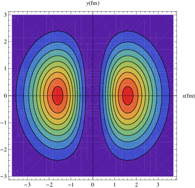
where , is the angle between and the -axis, and is the angle between and the -axis. Thus the transverse spin dependent density has an unusual cloverleaf shape. as shown in Fig. 2. Please see below for brief discussions about how shapes related to these can be measured and computed using lattice QCD techniques.
5 Model independent transverse charge density
In the infinite momentum frame the charge density operator becomes the plus-component of the current operator:
| (13) |
The light-cone “time”, . The separation can be defined only if an origin can be established. This is done by fixing the position of the transverse center-of-momentum to be , accomplished through the superposition of trasnverse momentum states:
| (14) |
The density itself is defined as the diagonal matrix element:
| (15) |
Using and the relation leads to the main result
| (16) |
This is the key result of the talk. The transverse charge density is the two-dimensional Fourier transform of the Dirac form factor, .
We begin the analysis by posing a motivational question. What is charge density at the center of the neutron? The neutron has no charge, but its charge density need not vanish. Is the central density positive or negative? According to an old idea presented by Fermi, a neutron sometimes fluctuates into a proton and a . The proton, as a heavy particle stays near the center, and the floats to the edge. This was evaluated more recently using the cloudy bag model Thomas et al. (1981). Another idea is that the repulsive one-gluon-exchange interaction between 2 quarks favors configurations with a positively charged quark at the center Friar (1972); Carlitz et al. (1977); Isgur et al. (1981). Both models suggest that the central region of the neutron is positively charged and both provide a function that rises a the value of increases from 0.
Here we avoid the use of models by analyzing the transverse charge density, . See figures 1,2 of Miller (2007b), which are shown here as Fig. 3 and Fig. 4.

Fig. 3 shows the surprising feature that the central charge density of the neutron is negative.
That the central charge density of the neutron is negative can be seen immediately from the negative-definite nature of the measured values of . The detailed structure of the neutron transverse charge density is also interesting, as shown in Fig. 4 The neutron transverse charge density is negative at the center, positive in the middle and negative at the outer edge. This suggests the presence of the pion cloud.

5.1 Explanation of the neutron’s negative central charge density
The negative nature of the central neutron charge density cries out for explanantion. This was attempted in different ways Miller and Arrington (2008); Rinehimer and Miller (2009a); Rinehimer and Miller (2009b) Ref. Miller and Arrington (2008) used generalized parton distributions, GPDs, to provide an interpretation. These are capable of yielding a three-dimensional picture of the nucleon in which one determines probability densities for a quark to be at a position and carry a given value of the longitudinal momentum transfer Burkardt (2003). For any given Fock-space component the relation
| (17) |
where the sum over is over the constituents in the component. This tells us that a quark carrying must be at a postion .
Various parameterizations Diehl et al. (2005); Guidal et al. (2005); Ahmad et al. (2007); Tiburzi et al. (2004) appear in the literature. The common theme is that deep inelastic scattering structure function and the elastic form factors follow the Drell-Yan Drell and Yan (1970) & West West (1970) relation:
| (18) |
The integer is one less than the number of valence quarks for a nucleon and the relation is that the same value of appears in the high momentum transfer form factor and the near unity behavior of the deep inelastic structure function. Thus large values of are related to large values of , which in turn means small values of . This connection between commuting position and momentum operators is not a conseqeunce of the uncertainty principle.
The negatively-charged quark dominates the large distribution of the neutron, Pumplin et al. (2002) and this which corresponds to small values of . Therefore it is natural to conclude that the central negative charge density arises from quarks at the center of the neutron Miller and Arrington (2008).
It is possible that these quarks arise from negatively charged pions that penetrate the interior of the nucleon. A simple model in which the neutron fluctuates into a proton and a , parametrized to reproduce the negative-definite nature of the neutron’s Rinehimer and Miller (2009b) reproduces the negative transverse central density. The change from the nominal, naive positive value of the charge density obtained from can be understood as originating in the boost to the infinite momentum frame Rinehimer and Miller (2009a).
6 Proton Magnetization density
The question of the location of the anomalous magnetization density of the proton was examined in Miller et al. (2008). The magnetization density was constructed by computing the matrix element of in a nucleon polarized in the -direction. The result obtained is that the anomalous magnetization density is given by
| (19) |
If one parameterizes the low form factors as
| (20) |
Ref. Miller et al. (2008) found that the mean square magnetization transverse radius is greater than the mean square transverse charge radius :
| (21) |
The question of the actual magnetization density was examined in Miller (2010) with the result that the actual magnetization density is . In either case the proton magnetization density extends further than its charge density.
7 Measuring the shape of the proton
The experiments capable of measuring the proton shapes reported above are studied in Miller (2008). The field-theoretic spin-dependent density is related to the transverse momentum distribution TMD, . TMDs are defined generally through the relations Mulders and Tangerman (1996)
| (22) |
where is an appropriate gauge link-operator and specifically we use
| (23) |
as the light-front version of the spin-dependent density. Here . The relation with an equal-time density operator is achieved by integrating the above quantities over . This sets so that .
The quantity can be measured using polarized electrons in the reaction . Other reactions can be used also; see the references in Miller (2008). If , the proton is not round.
8 Computing the shape of the proton using lattice QCD
One can define general model-independent densities Diehl and Hagler (2005) by considering matrix elements of the form , where is a Dirac matrix. The choice of corresponding to the spin-dependent density discussed earlier is where is an arbitrary vector representing the direction of the quark spin. Evaluating the matrix element of this quantity produces the spin-dependent density, which can be thought of as the integrated version of the coordinate space results of Miller (2003). The proton is non-spherical if the function of Gockeler et al. (2007) is non-vanishing, as recent lattice calculations show Schierholz (2009). Thus the proton is not round.
9 Summary
We have tried to explain how elastic and deep inelastic electron scattering can be analyzed from a unified light=front frame work using transverse charge densities, generalized parton distribution and transverse momentum distributions. Key physics results are that the neutron central charge density is negative, the proton magnetization density extends further than its charge density and that future experiments can determine whether or not the proton is round, as predicted by models Miller (2003) and QCD Schierholz (2009) by extracting the quantity .
References
- Frank et al. (1996) M. R. Frank, B. K. Jennings, and G. A. Miller, Phys. Rev. C54, 920–935 (1996), nucl-th/9509030.
- Miller (2003) G. A. Miller, Phys. Rev. C68, 022201 (2003), nucl-th/0304076.
- Miller (2007a) G. A. Miller, Phys. Rev. C76, 065209 (2007a), 0708.2297.
- Hofstadter (1956) R. Hofstadter, Rev. Mod. Phys. 28, 214–254 (1956).
- Bloom et al. (1969) E. D. Bloom, et al., Phys. Rev. Lett. 23, 930–934 (1969).
- Sachs (1962) R. G. Sachs, Phys. Rev. 126, 2256–2260 (1962).
- Miller (2009) G. A. Miller, Phys. Rev. C80, 045210 (2009), 0908.1535.
- Miller and Tiburzi (2009) G. A. Miller, and B. C. Tiburzi, Phys. Rev. C (submitted) (2009), 0911.3691.
- Perdrisat et al. (2007) C. F. Perdrisat, V. Punjabi, and M. Vanderhaeghen, Prog. Part. Nucl. Phys. 59, 694–764 (2007), hep-ph/0612014.
- Miller and Frank (2002) G. A. Miller, and M. R. Frank, Phys. Rev. C65, 065205 (2002), nucl-th/0201021.
- Jones et al. (2000) M. K. Jones, et al., Phys. Rev. Lett. 84, 1398–1402 (2000), nucl-ex/9910005.
- Gayou et al. (2002) O. Gayou, et al., Phys. Rev. Lett. 88, 092301 (2002), nucl-ex/0111010.
- Kvinikhidze and Miller (2006) A. Kvinikhidze, and G. A. Miller, Phys. Rev. C73, 065203 (2006), nucl-th/0603035.
- Miller (2008) G. A. Miller, Nuclear Physics News 18, 12–16 (2008), 0802.3731.
- Thomas et al. (1981) A. W. Thomas, S. Theberge, and G. A. Miller, Phys. Rev. D24, 216 (1981).
- Friar (1972) J. L. Friar, Part.Nucl. 4, 153–157 (1972).
- Carlitz et al. (1977) R. D. Carlitz, S. D. Ellis, and R. Savit, Phys. Lett. B68, 443 (1977).
- Isgur et al. (1981) N. Isgur, G. Karl, and D. W. L. Sprung, Phys. Rev. D23, 163 (1981).
- Miller (2007b) G. A. Miller, Phys. Rev. Lett. 99, 112001 (2007b), 0705.2409.
- Kelly (2004) J. J. Kelly, Phys. Rev. C70, 068202 (2004).
- Bradford et al. (2006) R. Bradford, A. Bodek, H. S. Budd, and J. Arrington, Nucl. Phys. Proc. Suppl. 159, 127–132 (2006), hep-ex/0602017.
- Miller and Arrington (2008) G. A. Miller, and J. Arrington, Phys. Rev. C78, 032201 (2008), 0806.3977.
- Rinehimer and Miller (2009a) J. A. Rinehimer, and G. A. Miller, Phys. Rev. C80, 015201 (2009a), 0902.4286.
- Rinehimer and Miller (2009b) J. A. Rinehimer, and G. A. Miller, Phys. Rev. C80, 025206 (2009b), 0906.5020.
- Burkardt (2003) M. Burkardt, Int. J. Mod. Phys. A18, 173–208 (2003), hep-ph/0207047.
- Diehl et al. (2005) M. Diehl, T. Feldmann, R. Jakob, and P. Kroll, Eur. Phys. J. C39, 1–39 (2005), hep-ph/0408173.
- Guidal et al. (2005) M. Guidal, M. V. Polyakov, A. V. Radyushkin, and M. Vanderhaeghen, Phys. Rev. D72, 054013 (2005), hep-ph/0410251.
- Ahmad et al. (2007) S. Ahmad, H. Honkanen, S. Liuti, and S. K. Taneja, Phys. Rev. D75, 094003 (2007), hep-ph/0611046.
- Tiburzi et al. (2004) B. C. Tiburzi, W. Detmold, and G. A. Miller, Phys. Rev. D70, 093008 (2004), hep-ph/0408365.
- Drell and Yan (1970) S. D. Drell, and T.-M. Yan, Phys. Rev. Lett. 24, 181–185 (1970).
- West (1970) G. B. West, Phys. Rev. Lett. 24, 1206–1209 (1970).
- Pumplin et al. (2002) J. Pumplin, et al., JHEP 07, 012 (2002), hep-ph/0201195.
- Miller et al. (2008) G. A. Miller, E. Piasetzky, and G. Ron, Phys. Rev. Lett. 101, 082002 (2008), 0711.0972.
- Miller (2010) G. A. Miller, Ann. Rev. Nuc. Part. Sci. 60 (2010).
- Mulders and Tangerman (1996) P. J. Mulders, and R. D. Tangerman, Nucl. Phys. B461, 197–237 (1996), hep-ph/9510301.
- Diehl and Hagler (2005) M. Diehl, and P. Hagler, Eur. Phys. J. C44, 87–101 (2005), hep-ph/0504175.
- Gockeler et al. (2007) M. Gockeler, et al., Phys. Rev. Lett. 98, 222001 (2007), hep-lat/0612032.
- Schierholz (2009) G. Schierholz, Workshop on Transverse partonic Structure of Hadrons,2009 (2009).