Direct imaging with highly diluted apertures. II: Properties of the point spread function of a hypertelescope

Direct imaging with highly diluted apertures. II: Properties of the point spread function of a hypertelescope–References2008

F. Patru Affiliation: Laboratoire H. FIZEAU, UMR CNRS 6525 - UNS, OCA - Avenue Copernic, 06130 Grasse, France Affiliation: Laboratoire d’Astrophysique de Grenoble (LAOG), 414 Rue de la Piscine, Domaine Universitaire, 38400 Saint-Martin d’Hères, France N. Tarmoul Affiliation: Laboratoire H. FIZEAU, UMR CNRS 6525 - UNS, OCA - Avenue Copernic, 06130 Grasse, France D. Mourard Affiliation: Laboratoire H. FIZEAU, UMR CNRS 6525 - UNS, OCA - Avenue Copernic, 06130 Grasse, France O. Lardière Affiliation: Adaptive Optics Lab, Engineering Lab Wing B133, University of Victoria, PO Box 3055 STN CSC, Victoria, BC, Canada V8W 3P6

Accepted. Received

Abstract

In the future, optical stellar interferometers will provide true images thanks to larger number of telescopes and to advanced cophasing subsystems. These conditions are required to have sufficient resolution elements (resel) in the image and to provide direct images in the hypertelescope mode. It has already been shown (Lardiere et al., 2007) that hypertelescopes provide snapshot images with a significant gain in sensitivity without inducing any loss of the useful field of view for direct imaging applications. This paper aims at studying the properties of the point spread functions of future large arrays using the hypertelescope mode. Numerical simulations have been performed and criteria have been defined to study the image properties. It is shown that the choice of the configuration of the array is a trade-off between the resolution, the halo level and the field of view. A regular pattern of the array of telescopes optimizes the image quality (low halo level and maximum encircled energy in the central peak), but decreases the useful field of view. Moreover, a non redundant array is less sensitive to the space aliasing effect than a redundant array.

Keywords:

Instrumentation: high angular resolution – Instrumentation: interferometers – Telescopes – Methods: observational

Refer to caption — Figure 1: Field of view and direct imaging in hypertelescope mode. An example of an input pupil (top-left) and a densified pupil (middle-left) is shown. We have represented the (u,v) plane coverage (bottom-left) considering that the finite size of the individual telescopes has been neglected. It can be seen that the high spatial frequencies are distributed over the interval $[s/\lambda,B/\lambda]$ , with $s$ the smallest baseline and $B$ the largest baseline of the array. The maximum densification factor $\gamma_{max}$ equals to $s/d_{i}$ (bottom-right). The Fizeau (top-right) and densified (middle-right) point spread functions (PSF) are shown. As predicted, we observe a central peak inside a clean zone, called the Clean Field ( $CLF$ ), where the contribution of the side-lobes’halo is minor (see (Lardiere et al., 2007) for the different definitions of fields). It is surrounded by a non-negligible halo of speckles outside the $CLF$ diameter ( $CLF=\lambda/s$ ). The Fizeau PSF is limited by the Airy envelope of an input sub-aperture, which corresponds to the coupled field ( $CF=\lambda/d_{i}$ ). The pupil densification reduces the Direct Imaging Field (DIF) to match the CLF. The central peak is intensified by a factor $\gamma^{2}$ .

1 Introduction

Future large interferometers (Labeyrie, 2008) need a large number of telescopes and an active cophasing system, to provide images with sufficient sensitivity. If both conditions are met, snapshot imaging can be used in the hypertelescope mode (Labeyrie, 1996) and a multi-axial beam combiner seems to be the best solution. If the entrance pupil is highly diluted, the hypertelescope mode improves the Fizeau mode, with a high sensitivity gain without any loss of the useful field of view for direct imaging applications. This useful field, where a direct image can be correctly recovered, is called the Clean Field (Lardiere et al., 2007).

Direct imaging has two main features. In a conventional sense, the goal is to provide snapshot images that could then be post-processed by deconvolution techniques. These images give valuable regularization constraints for the a posteriori astrophysical analysis process. Furthermore, direct imaging is well suitable to feed the entrance plane of focal instruments such as coronagraphic devices or integral field spectrometer. In this paper, we concentrate our analysis on the raw images without considering the deconvolution techniques or the coupling with a focal instrument.

Keeping in mind the researches on the ways to optimize the imaging capabilities of a hypertelescope, this paper aims at characterizing the point spread functions of typical future large arrays. For this purpose, we have developed a numerical simulation, called HYPERTEL, which first simulates direct images (Sect. 2) and then analyses the densified PSF properties by defining different quantitative criteria (Sect. 3). Then, we study the impact of the array configuration (geometry of the array and number of apertures) and of the recombination mode (Sect. 4). Finally, we establish the relations between the astrophysical parameters of the science object and the main parameters of the hypertelescope (Sect. 5).

2 Simulating direct images

2.1 The input parameters

The input parameters are the wavelength, the characteristics of the science object, the array configuration and the recombination mode.
We assume a perfectly cophased array, without any degradation in the image due to atmospheric turbulence or instrumental bias. To simplify the study, we restrict ourselves to the monochromatic case.

2.1.1 The array configuration

The array is made of $N_{T}$ identical sub-apertures of index $k$ , defined by their positions $(u_{p}(k),v_{p}(k))$ in the input pupil plane and by their diameter $d_{i}$ . We note $s$ (resp. $B$ ) the smallest (resp. largest) baseline of the array. The maximum angular resolution of the array, following the Rayleigh criterion, is given by the highest baseline :

resel\simeq\frac{\lambda}{B}

(1)

2.1.2 The science object

The object is defined by a monochromatic brightness map, $N_{pxl}$ pixels wide. The angular extent of this map is equal to the object diameter $\theta_{obj}$ . The angular size of a pixel $\theta_{pxl}$ , i.e. the smallest angular element seen on the sky, should respect the Shannon criterion:

\theta_{pxl}=\frac{\theta_{obj}}{N_{pxl}}<\frac{resel}{2}

(2)

In practice, we choose $\theta_{pxl}<resel/6$ .

Thus, $N_{pxl}>\frac{6B}{\lambda}\cdot\theta_{obj}$ .

The object is considered as composed of elementary incoherent sources, corresponding to the $N_{pxl}^{2}$ pixels of the brightness map. Each elementary source of index $m$ is defined by its coordinates $(X_{obj}(m),Y_{obj}(m))$ and by its intensity $I_{obj}(m)$ .

For each elementary source, the off-axis position is defined on the two axis by:

	$\displaystyle\theta_{X\,obj}(m)=\left(X_{obj}(m)-\frac{N_{pxl}}{2}\right)\,\theta_{pxl}$
	$\displaystyle\theta_{Y\,obj}(m)=\left(Y_{obj}(m)-\frac{N_{pxl}}{2}\right)\,\theta_{pxl}$		(3)

The image is obtained as the sum of the sub-images of each incoherent elementary source. As the input sub-pupils are very diluted, we neglect the variation of the object in the spatial frequency domains [ $\frac{B-d_{i}}{\lambda}$ ; $\frac{B+d_{i}}{\lambda}$ ] accessible in certain recombination schemes.

2.1.3 The recombination mode

Pupil densification increases by a factor $\gamma$ the relative size of the beams and keeps the relative positions of the sub-pupil centres (Fig. 1). This pseudo-homothetic transformation does not affect the interferometric pattern in the image and correctly recovers the high resolution information. The diffraction envelope is reduced, so as to concentrate all the flux in the useful field.

The alternative concept of IRAN (Vakili et al. 2004a, ) combines the beams by superimposing the images of the sub-pupils with small tilts in the image plane. A direct image is obtained in the recombined pupil plane.

The envelope shape is a Bessel function in Pupil Densification (DP mode) and is a flat field in IRAN mode. The envelope width decreases as the densification factor increases. The value of the latter is chosen between 1 (Fizeau mode) and $\gamma_{max}$ (maximum densification).

The maximum densification factor depends on the smallest baseline $s$ and on the aperture diameter $d_{i}$ :

\gamma_{max}=\frac{s}{d_{i}}

(4)

The pupil densification amplifies the intensity of the signal by a factor $\gamma^{2}$ . In the IRAN mode, the densification factor can not be larger than $\gamma_{max}/2$ due to the diffraction of the sub-pupils (Lardiere et al., 2007). Thus the sensitivity gain is reduced by a factor 4 and the DIF is enlarged by a factor 2, compared to the DP mode.

We mainly focus in this paper on the pupil densification (DP) for the recombination mode. We also make comparison with the image densification (IRAN).

2.2 The image calculation

The principle of the image calculation is schematically described in Fig. 2. In the image plane, each pixel of coordinates $(x,y)$ has an intensity of $I(x,y)$ .

The Point Spread Function (Lardiere et al., 2007) is defined as the product of the interference function $I_{0}(x,y)$ (function of the array pattern) with the diffraction envelope $A_{0}(x,y,\gamma)$ (function of the recombination mode and of the densification factor).

I_{PSF}(x,y)\approx A_{0}(x,y,\gamma)\times I_{0}(x,y)\ ,

(5)

with:

I_{0}(x,y)=\bigg|\sum_{k=1}^{N_{T}}\,e^{\frac{-2i\pi}{\lambda}(x\cdot u_{p}(k)+y\cdot v_{p}(k))}\bigg|^{2}\\

(6)

The direct image of an astrophysical object is defined as the object brightness distribution $O(\theta_{X\,obj},\theta_{Y\,obj})$ convolved by the interference function, the result being multiplied by the diffraction envelope.

I(x,y)\approx A_{0}(x,y,\gamma)\cdot O(\theta_{X\,obj},\theta_{Y\,obj})\otimes I_{0}(x,y)\,\\

(7)

Finally, the image computed by HYPERTEL is the sum of the sub-images of each incoherent elementary source of the object (as defined in Sect. 2.1.2).

	$\displaystyle I(x,y)=A_{0}(x,y,\gamma)\cdot\bigg\|\sum_{k=1}^{N_{T}}\,e^{\frac{-2i\pi}{\lambda}(x\cdot u_{p}(k)+y\cdot v_{p}(k))}\cdot$
	$\displaystyle\sum_{m=1}^{N_{pxl}^{2}}\,I_{obj}(m)\cdot e^{\frac{2i\pi}{\lambda}\psi(m,k)}\bigg\|^{2}$		(8)

We denote $\psi(m,k)$ the phase delay seen by the $k^{th}$ sub-aperture due to the position of the elementary source $m$ . Indeed each elementary source is seen under a different angle by each sub-aperture of the interferometer. Hence, $\psi(m,k)$ is given by:

\psi(m,k)=\theta_{X\,obj}(m).u_{p}(k)+\theta_{Y\,obj}(m).v_{p}(k)

(9)

3 Definition of the characteristics of the point spread function (PSF)

3.1 Input and output pupils’ parameters

As the computed images are a function of the characteristics of the entrance pupil, we first define two parameters related to the interferometer configuration. The entrance (resp. densified) pupil filling rate $\tau_{i}$ (resp. $\tau_{o}$ ) is defined as the ratio between the total surface area of the input (resp. output) pupil and the surface area of an input (resp. output) sub-pupil, $d_{i}$ (resp $d_{o}$ ) being the diameter of the latter:

\tau_{i}=\frac{S_{input~sub-pupils}}{S_{input~pupil}}=N_{T}\frac{d_{i}^{2}}{(B+d_{i})^{2}}

(10)

\tau_{o}=\frac{S_{output~sub-pupils}}{S_{output~pupil}}=N_{T}\frac{d_{o}^{2}}{(B+d_{o})^{2}}=N_{T}\left(\frac{\gamma\,d_{i}}{B+\gamma\,d_{i}}\right)^{2}

(11)

3.2 Field of view parameters

The definitions of the different fields of view for a hypertelescope have been extensively studied by Lardiere et al. (2007). We just recall here the important definitions of these different fields. We distinguish the CLean Field of view (CLF), the Direct Imaging Field of view (DIF) and the Coupled field of view (CF). They are illustrated on figure 1.

CLF=\frac{\lambda}{s}\,(radians)\,=\frac{B}{s}\,(resels)\\

(12)

DIF\simeq\frac{\lambda}{(\gamma-1)\>d_{i}}\\

(13)

CF=\frac{\lambda}{d_{i}}\\

(14)

The Clean Field is physically related to the sampling of the (u,v) plane and according to Nyquist-Shannon sampling theorem, it is defined by the smallest baseline $s$ . This definition is also interesting on calculating the number of resels in the Clean Field.

The coupled field (CF) is imposed by the size of a sub-aperture. The Direct Imaging Field (DIF) depends on the densification mode. The DIF width is still obviously smaller than the CF width.

3.3 Astrometric criteria

In the direct image, the position of each interference peak (central peak and side-lobes) is given by the coordinates of its photocentre (Fig. 3). The full width at half maximum (FWHM) of the central peak corresponds to the smallest resolution element (resel), given by equation 1. It characterizes the sharpness of the image. It depends not only on the wavelength and on the maximum baseline, but also on the geometry of the array.

3.4 Photometric criteria

The on-axis intensity $I_{0}$ is equal to the height of the central peak. The encircled energy is defined as the ratio of the fraction of energy contained in the central peak $E_{0}$ to the total energy in the image $E_{tot}$ :

\frac{E_{0}}{E_{tot}}=\frac{2\pi}{E_{tot}}\int_{0}^{\theta_{0}}I(\rho)\,\rho\,d\rho

(15)

where $\theta_{0}$ corresponds to the first minimum from the center of the field (Fig. 3).

3.5 Halo level criteria

We also define a criterion to estimate the contribution of the halo surrounding the central peak. The maximum of the halo level is defined as the ratio between $I_{1}$ the intensity of the highest side-lobe inside the CLF and $I_{0}$ the intensity of the central peak (Fig. 3).

Maximum~halo~level\,=\,\frac{I_{1}}{I_{0}}

(16)

4 Densified PSF properties

4.1 Influence of the array geometry

4.1.1 Presentation of the simulations

We consider four typical array configurations, made of 40 telescopes, 10m in diameter and distributed over a maximum baseline of 1km with $\lambda$ =0.6 $\mu$ m. The distribution of the pupils is taken from ELSA (Quirrenbach, 2004), OVLA (Labeyrie et al., 1986), KEOPS (Vakili et al. 2004b, ) and CARLINA (Labeyrie et al., 2003). Figure 4 and Table 1 give the characteristics of the PSFs and compare the cases of pupil densification (DP mode) and image densification (IRAN mode (Vakili et al. 2004a, )).

OVLA and ELSA have an almost uniform coverage of the (u,v) plane and a large clean field (10 and 18 resels respectively). OVLA has diffraction rings and ELSA has diffraction spikes inside the clean field, so that only $12\%$ of the energy is contained inside the central peak. The maximum halo level corresponding to the diffraction structures reaches $16\%$ (resp. $22\%$ ) of the amplitude of the central peak for OVLA (resp. ELSA).

KEOPS and CARLINA have a uniform coverage of the input pupil, so that the coverage of the output pupil is maximized. The densified pupil filling rate reaches $75\%$ (resp. $69\%$ ) for KEOPS (resp. CARLINA). The minimal distance between the telescopes is also optimized, so that the clean field is reduced to about $5$ resels. The advantage is an improvement of the image quality, so that the encircled energy reaches $71\%$ (resp. $65\%$ ) for KEOPS (resp. CARLINA), whereas the maximum halo level remains below $3\%$ .

		CARLINA-37	KEOPS-40	OVLA-39	ELSA-39
Entrance pupil filling rate	$\tau_{i}$	3.6e-3	3.9e-3	3.8e-3	3.8e-3
Densified pupil filling rate	$\tau_{o}$	0.69	0.75	0.22	0.07
Maximum densification level	$\gamma_{max}$	15.8	15.8	8.1	4.4
Clean field [mas]	CLF	0.78	0.78	1.54	2.79
Clean field [resel]	CLF	5.18	5.18	10.18	18.45
Direct imaging field [resel]	DIF	5.53	5.53	11.62	23.82
FWHM of the central peak [resel]	$FWHM$	0.73	0.70	0.55	0.89
Encircled energy of the central peak	$E_{0}/E_{tot}$	0.71	0.65	0.12	0.12
Maximum halo level in the CLF	$I_{1}/I_{0}$	0.03	0.02	0.16	0.22

Table 1: Imaging parameters of 4 array configurations of 40 telescopes. The aperture diameters are equal to

10m

and the maximum baseline is

1km

, so that the

resel

0.12~mas

and the Coupled Field

CF

82~resels

4.1.2 Trade-off between halo level and field of view

For a given resolution, it appears that, depending on the chosen configuration, there is a trade-off between halo level and field of view. OVLA is suitable to image large fields, since the corresponding diffraction envelope (dashed line) has a large full width at half maximum. KEOPS and CARLINA are optimized for high contrast imaging, thanks to a regular distribution of the telescopes of the array.

The condition to reach a low halo level with a monolithic telescope is to have an aperture without obstruction, or to use apodization techniques (Aime and Soummer 2003a, ). In these conditions, the (u,v) plane coverage has a conic shape. In a similar way, the (u,v) plane of an interferometer used for high contrast imaging must be identical. It has been shown that the optimization of the filling of the (u,v) plane is obtained by maximizing the integral of the squared modulus of the Modulation Transfer Function (Aime and Soummer 2003b, ). It consists in fact in maximizing the densified pupil filling rate $\tau_{o}$ (Eq. 11), by a regular distribution of the sub-pupils.

4.1.3 Trade-off between resolution and field of view

For a given configuration, it appears also that there is a trade-off between resolution and field. If one increases the global size of the input pupil ( $B$ ) with a constant number of apertures, the resolution is improved whereas the clean field is decreased. A compact array provides a large image with low resolution and a diluted array provides a sharp image with high resolution. It is interesting to benefit from a movable array with a fixed geometry like KEOPS and with a sufficient number of telescopes. With a small number of iterations, the telescopes could be moved keeping the same geometry so as to finally adapt the CLean Field to the typical dimension of the object.

4.2 Impact of the number of apertures

		KEOPS-8	KEOPS-21	KEOPS-40	KEOPS-65	KEOPS-96
Entrance pupil filling rate	$\tau_{i}$	0.78e-3	2.1e-3	3.9e-3	6.4e-3	9.4e-3
Densified pupil filling rate	$\tau_{o}$	0.76	0.75	0.75	0.75	0.74
Maximum densification level	$\gamma_{max}$	44.5	23.3	15.8	12.0	9.6
Clean field [mas]	$CLF$	0.28	0.53	0.78	1.03	1.28
Clean field [resel]	$CLF$	1.84	3.52	5.18	6.83	8.49
Direct imaging field [resel]	$DIF$	1.88	3.67	5.53	7.46	9.47
Full-width half-maximum [resel]	$FWHM$	0.56	0.66	0.70	0.72	0.74
Encircled energy of the central peak	$E_{0}/E_{tot}$	0.66	0.67	0.69	0.72	0.73
Maximum halo level (inside the CLF)	$I_{1}/I_{0}$	0.03	0.02	0.02	0.02	0.02
		OVLA-9	OVLA-21	OVLA-39	OVLA-69	OVLA-96
Entrance pupil filling rate	$\tau_{i}$	0.88e-3	2.1e-3	3.8e-3	6.7e-3	9.4e-3
Densified pupil filling rate	$\tau_{o}$	0.60	0.36	0.22	0.13	0.10
Maximum densification level	$\gamma_{max}$	34.8	14.9	8.1	4.6	3.3
Clean field [mas]	CLF	0.36	0.83	1.54	2.72	3.78
Clean field [resel]	CLF	2.36	5.48	10.18	18.0	25.1
Direct imaging field [resel]	DIF	2.43	5.88	11.62	23.1	36.1
Full-width half-maximum [resel]	$FWHM$	0.53	0.55	0.55	0.55	0.55
Encircled energy of the central peak	$E_{0}/E_{tot}$	0.42	0.20	0.11	0.07	0.05
Maximum halo level (inside the CLF)	$I_{1}/I_{0}$	0.13	0.16	0.16	0.16	0.16

Table 2: Imaging parameters of the configurations KEOPS (upper part) and OVLA (lower part) as a function of the number of telescopes. The aperture’s diameter is

10m

and the maximum baseline

1km

, so that the

resel

0.12~mas

and the Coupled Field

CF

82~resels

4.2.1 Presentation of the simulations

We now consider the same four array configurations but with a variable number of telescopes (up to 100) of diameter $10m$ distributed over a constant maximum baseline of $1km$ .

In order to keep the geometry of each configuration, we use the following principles for computing the different arrays:

•

ELSA : at each step, we add one telescope on each arm of the Y, starting at 3 telescopes, then 6 and up to 99.
•

OVLA : at each step, 1 telescope is added on the ring with a diameter of 1 km, starting at 2 telescopes, then 3 and up to 100. The telescopes are regularly distributed in azimuth.
•

KEOPS : we start with a telescope at the centre and one concentric ring of 7 telescopes. Then we add successively concentric rings made of 13, 19, 25 and 31 telescopes. The array is successively composed of 8 (1 ring), 21 (2 rings), 40 (3 rings), 65 (4 rings) and 96 (5 rings) telescopes. The diameter of the largest ring always equals 1 km.
•

CARLINA : at each step, the array is build with $n^{2}$ telescopes regularly distributed over a square grid, with $n$ from 2 to 11. The telescopes outside the circle of diameter $B$ are removed. The array is composed successively of 4, 9, 12, 21, 32, 37, 52, 69, 80 and 97 telescopes.

The intensity is normalized by the collecting surface area of each array so that the sensitivity considered here is independent of the number of telescopes.

4.2.2 PSF quality parameters

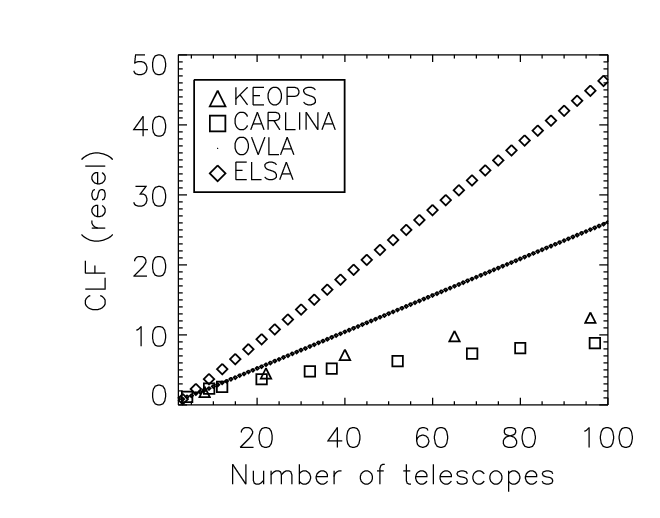
Figure 5 shows the densified pupils and the interference function (as defined in Eq. 6) of the four configurations with 20 and 100 telescopes. Figure 6 and Table 2 give the evolution of the main parameters of the arrays as a function of the number of telescopes. Figure 7 gives the evolution of the densified PSF parameters as a function of the number of telescopes for each configuration. Figure 8 shows the correlation between the PSF parameters and the densified pupil filling rate.

Whatever the number of telescopes, CARLINA and KEOPS benefit from a quasi-complete densified pupil filling rate, so that their imaging properties (inside the clean field) are very close to a monolithic telescope. The encircled energy in the central peak contains about $70\%$ of the luminous energy and the contribution of the halo remains below $3\%$ inside the clean field. CARLINA and KEOPS are a priori equivalent in term of image quality, regarding to the halo level and the encircled energy.

For OVLA and ELSA, the output pupil shape is similar whatever the number of telescopes. When the number of telescopes increases in these arrays, the densification level remains low due to the shortest baselines. The encircled energy in the central peak falls from $40\%$ to only $5\%$ , regarding the configurations from 10 to 100 telescopes. The halo level is not negligeable for ELSA (20 $\%$ ) and OVLA (15 $\%$ ).

The sharpness of the image is characterized by the FWHM of the central peak. The narrowest peak is provided by OVLA, thanks to the huge central obstruction of the input pupil. ELSA exhibits strong diffraction spikes but the PSF looks very sharp in the other position angles. For KEOPS and CARLINA, the FWHM of the central peak increases slowly with the number of telescopes.

5 Biases induced on the PSF

In the previous section, we have studied various configurations of future arrays. This study has allowed us to characterize them with quantitative parameters. It appears clearly that, whatever the configuration, the imaging properties will be degraded by difficulties in restoring the photometric parameters in the field. Three main effects are identified:

•

the bias of the interference function,
•

the space aliasing effect,
•

the bias of the diffraction envelope.

The two first depend on the array configuration, whereas the last bias is only related to the recombination mode.

5.1 Bias of the interference function

The photometric parameters of a source are biased by the halo of the interference function (as defined in Eq. 6), which induces a contrast loss in the image. The quality of the interference function of the array is simply related to the actual shape of the entrance pupil.

If the input sub-pupils are distributed regularly, the densified pupil is almost complete, and the halo inside the clean field reproduces the diffraction pattern of a large monolithic telescope covering all the sub-pupils. If the densified pupil shows gaps, additional diffraction figures are added to first ones.

Thus, the halo is minimized by maximizing the densified pupil filling rate $\tau_{o}$ , with a regular pattern of the sub-apertures in the entrance pupil.

5.2 Space aliasing effect

The space aliasing effect (Aime, 2008) appears in the direct image when the science object is surrounded by sources outside the clean field but inside the coupled field, or when the science object diameter is larger than the clean field. Besides, all the sources in the CF will contribute to the central image but only the sources in the CLF will form a correct central peak plus a halo of sidelobes, whereas the sources in the CF and outside the CLF will just form a halo of sidelobes. These side-lobes induce photometric perturbations locally distributed in the image.

Redundant arrays are more affected by the space aliasing effect than non redundant arrays. Indeed, a redundant array provides an interference function with high level parasit peaks, whereas a non redundant one has a smooth interference function . In the image formation, these differences in the interference functions will introduce important space aliasing effects as shown on Fig. 9 and 10.

In the redundant case, a source in the Coupled Field but outside the Clean Field provides ghost images inside the Clean Field. In the non redundant case, the same star will only induce a diffused halo reducing the contrast in the Clean Field.

5.3 Bias of the diffraction envelope

Due to the diffraction envelope contribution, the quality of the photometry restitution decreases from the axis to the edge of the clean field (Fig. 10). A partial densification restitutes a more homogeneous photometry in the clean field, but decreases the sensitivity gain. This bias does not exist in IRAN mode, where the envelope is flat.

5.4 Discussion

The main effects on the PSF can be theoretically corrected by image restoration or deconvolution. Deconvolution techniques are required for complex objects. In the case of a densified image, the problem is that the convolution relationship is lost. The image and the PSF are in fact partially truncated, which is a problem for the classical methods of deconvolution. To overcome this problem, a hybrid method, based on likelihood maximization, reconstructing simultaneously the object and the PSF has been proposed (Aristidi et al., 2006).

Figure 11 gives the links between the science object and the hypertelescope’s required characteristics. An astrophysical object is characterized by its dimensions, its complexity and its brightness. These characteristics are linked to the main parameters of a hypertelescope: field, resolution, pupil pattern.

The main dimensions of the object are the external diameter and the smallest resel of interest. The maximum size of the object should not exceed the diameter of the clean field, which leads to the value of the minimum baseline of the array ( $CLF=\lambda/s$ ). The smallest resel corresponds to the required resolving power, which imposes the largest baseline B of the array ( $resel=\lambda/B$ ). The clean field can also be expressed in number of resels ( $CLF=B/s$ ).

The complexity of the object determines the required number of resels in the image, the number of telescopes and the array geometry. The other aspect to be considered is the resolution range of the object on the interval $[\lambda/B,\lambda/s]$ .

The limiting magnitude of an array is directly related to the performances of the cophasing device, allowing long exposures. The image quality (highest encircled energy in the central peak and lowest halo level in the CLean Field) is directly related to the densified pupil filling rate.

6 Conclusion

Simulations have shown that the choice of the array configuration (array pattern and number of apertures) is a trade-off between the resolution, the halo level and the useful field. The spatial resolution is given by the largest baseline ( $resel=\lambda/B$ ). The clean field is a function of the smallest baseline ( $CLF=\lambda/s$ ). The halo level and the encircled energy in the central peak are a function of the densified pupil filling rate $\tau_{o}$ . The sine qua none condition to image a complex source without space aliasing effect is that the object diameter should not exceed the clean field width ( $\theta_{obj}<\lambda/s$ ).

Concerning the beam combiner, it has been shown that the maximum densification is optimal in term of sensitivity, by equalizing the direct imaging field (DIF) with the clean field.

Simulations have shown that the configurations KEOPS and CARLINA are equivalent as regards the image characteristics. However, KEOPS is less sensitive to the space aliasing effect, contrary to CARLINA where ghost stars are introduced by the pollution of the surrounding sources. Thus, a non redundant array is required for Direct Imaging to minimize the space aliasing effect.

Finally, the best configuration seems to be the one proposed by KEOPS, which has a regular and non redundant layout of the telescopes. This configuration provides the best quality of the interference function, in comparison with the interference function of the equivalent giant telescope. Indeed, it provides the lowest halo level (inside the Clean Field), at the limit of the diffraction of such kind of array. Moreover, minimizing the halo level improves the signal to noise ratio, which should simplify the deconvolution process.

Thus, a KEOPS configuration seems to be suited for high-contrast imaging of compact sources. An OVLA configuration can be used for wide field imaging, providing a larger clean field and the best resolving power.

This paper was mainly focused on future large arrays with a large number of sub-apertures. However, the direct imaging technique already has a great interest for current operating interferometers, using an efficient cophasing system. Indeed, the densification may provide the ultimate sensitivity.

It will be also interesting in the future to compare the performances of direct imaging and aperture synthesis. The introduction of the fundamental and instrumental noises is also mandatory for a correct evaluation of the scientific performances. Finally this work will be developed in two main directions: the study of the instrumental performances of direct imaging arrays when coupled with integral field spectrometers or coronagraphs, and the comparison of the practical imaging performances of various array configurations when deconvolution is applied.

Acknowledgments

The authors wish to thank the referee, Chris Haniff, for important suggestions and clarifications.

References

(1) Aime C. and Soummer R. 2003, Astronomy with High Contrast Imaging, EAS Publications Series, 8, 79
(2) Aime C. and Soummer R. 2003, Astronomy with High Contrast Imaging, EAS Publications Series, 8, 353
Aime (2008) Aime C. 2008, A&A, 483, 361
Aristidi et al. (2006) Aristidi E., Vakili F., Schutz A. et al. 2006, EAS Publications Series, 22, 103
Labeyrie et al. (1986) Labeyrie A., Koechlin L. and Lemaitre G. 1986, Proc. SPIE, 628, 323
Labeyrie (1996) Labeyrie A., 1996, A&AS, 118, 517
Labeyrie et al. (2003) Labeyrie A., Le Coroller H., Dejonghe J. et al. 2003, Proceedings SPIE Hawaii 4852, 236-247
Labeyrie (2008) Labeyrie, A., 2008, ”ELTs, interferometers and hypertelescopes at different wavelengths”, proc. ”ELTs at different wavelengths”, SPIE Lund, in press
Lardiere et al. (2007) Lardiere O., Martinache F. and Patru F. 2007, Mon. Not. R. Astron. Soc. 375, 977
Patru et al. (2007) Patru F. et al. 2007 , MNRAS, 376, 1047
Quirrenbach (2004) Quirrenbach A. 2004, Science cases for next generation optical/infrared inteferometric facilities (the post VLTI era), Proc. of the 37th Liege International Astrophys. Colloquium, 43
(12) Vakili F., Aristidi E., Abe L. and Lopez B. 2004, A&A, 421, 147
(13) Vakili F., Belu A., Aristidi E. et al. 2004, Proc. SPIE, 5491, 1580

DP mode ( $\gamma=\gamma_{max}$ )	DP mode ( $\gamma=\gamma_{max/2}$ )	IRAN mode ( $\gamma=\gamma_{max/2}$ )