Energy Optimization across Training and Data for Multiuser Minimum Sum-MSE Linear PrecodingThanks: This work has been submitted to the IEEE for possible publication. Copyright may be transferred without notice, after which this version may no longer be accessible.

In the linear precoding system illustrated in Fig. 1, a base station with $M$ antennas transmits to $K$ decentralized mobile users with $N_{k}$ antennas each over flat wireless channels.

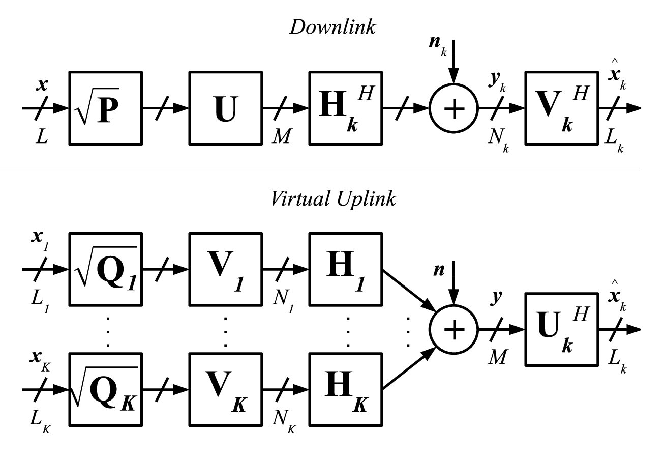
The channel between the transmitter and user $k$ is represented by the $N_{k}\times M$ matrix $\mathbf{H}_{k}^{H}$, and the overall $N\times M$ channel matrix is $\mathbf{H}^{H}$, with $\mathbf{H}=\left[\mathbf{H}_{1},\dots,\mathbf{H}_{K}\right]$, and where $N=\sum_{k}N_{k}$ is the total number of receive antennas in the system. We assume that all channel coefficients are i.i.d. and drawn from a zero-mean complex Gaussian distribution with variance $\sigma_{H}^{2}$; that is, $\mathrm{vec}(\mathbf{H})\sim\mathcal{CN}(\mathbf{0},\sigma_{H}^{2}\mathbf{I}_{MN})$. We consider a quasi-static (block fading) channel model, where the channel coefficients are assumed to be fixed for a coherence interval of $n$ consecutive symbol periods. The first $n_{T}$ transmissions in each block are training symbols which the mobile receivers use to estimate the downlink channel, $\hat{\mathbf{H}}_{k}^{H}$; these imperfect CSI estimates are assumed to be available at the base station via an error-free and delay-free feedback mechanism. We consider the stochastic error model (as used in [DingPhD, SD08, DB09]) where the true channel is modelled as a sum of the estimated channel and an independent additive error term, $\mathbf{H}_{k}=\hat{\mathbf{H}}_{k}+\mathbf{E}_{k}$ with $\mathrm{vec}(\mathbf{E}_{k})\sim\mathcal{CN}(\mathbf{0},\sigma_{k}^{2}\mathbf{I}_{MN_{k}})$, and $\mathbf{E}=\left[\mathbf{E}_{1},\dots,\mathbf{E}_{K}\right]$.

Training sequence and estimator design can be simplified under the assumption of uncorrelated channel coefficients by considering training for vector channels from the $M$ transmit antennas to each individual receive antenna. To simplify notation in this section, we consider training for a single vector channel $\mathbf{h}^{H}$. Channel estimation is performed by transmitting a set of $n_{T}$ training signal vectors, $\mathbf{X}_{T}=\left[\mathbf{x}_{T,1},\dots,\mathbf{x}_{T,n_{T}}\right]$, from the $M$ transmit antennas without precoding. $n_{T}\geq M$ training symbol vectors must be sent to guarantee resolvability of the individual channel coefficients. The received signal vector is $\mathbf{y}_{T}=\mathbf{h}^{H}\mathbf{X}_{T}+\mathbf{z}$, where $\mathbf{z}\sim\mathcal{CN}(\mathbf{0},\sigma_{n}^{2}\mathbf{I}_{n_{T}})$, and the MMSE channel estimate $\hat{\mathbf{h}}_{\mathrm{MMSE}}^{H}=\mathbf{y}_{T}\mathbf{A}_{0}$ is found using the linear MMSE estimator $\mathbf{A}_{0}=\left(\mathbf{X}_{T}^{H}\mathbf{X}_{T}+\frac{\sigma_{n}^{2}}{\sigma_{H}^{2}}\mathbf{I}_{n_{T}}\right)^{-1}\mathbf{X}_{T}^{H}$. Under the sum energy constraint, $\mathrm{tr}\left[\mathbf{X}_{T}^{H}\mathbf{X}_{T}\right]\leq E_{T}$, where $E_{T}$ is the energy allocated to training, and the assumption of independent channel coefficients, a sufficient condition for optimality of the training matrix is $\mathbf{X}_{T}\mathbf{X}_{T}^{H}=\frac{E_{T}}{M}\mathbf{I}_{M}$ [BG06]; that is, we are free to select any training matrix with orthogonal rows. When using the MMSE estimator, there is no benefit using any more than $n_{T}=M$ training symbols. For algorithmic simplicity, we choose the set of training vectors $\mathbf{X}_{T}=\sqrt{\frac{E_{T}}{M}}\mathbf{I}_{M}$. One may also choose $\mathbf{X}_{T}$ as the scaled size-$M$ DFT matrix, $\left[\mathbf{X}_{T}\right]_{m,n}=\frac{\sqrt{E_{T}}}{M}e^{-j2\pi mn/M}$, which has the additional benefit of balancing training power equally over each transmit antenna in each training symbol.

In Appendix A, we show that the estimation errors of each channel coefficient are equal under the assumption of i.i.d. channels with variance $\sigma_{H}^{2}$, taking the value

As we illustrate in Section II-D, the assumption of equal estimation error variance is critical in maintaining convexity of the virtual uplink sum-MSE minimization problem.

Following training, we assume that all of the remaining $n_{D}=n-M$ symbol periods in each block will be used to broadcast data symbols. Under the block fading assumption, the channel $\mathbf{H}$ does not change during these $n_{D}$ data transmissions; thus, we can design a single precoder/decoder pair to be used for all transmissions in the block. It follows that the remaining available energy to be used for data $(E_{D}=E_{\max}-E_{T})$ should be divided equally over the $n_{D}$ data transmissions, resulting in a maximum per-symbol transmit power $P_{D}=(E_{\max}-E_{T})/n_{D}$.

During each data transmission, user $k$ receives $L_{k}$ data symbols $\mathbf{x}_{k}=\left[x_{k1},\dots,x_{kL_{k}}\right]^{T}$ from the base station, and the vector $\mathbf{x}=\left[\mathbf{x}_{1}^{T},\dots,\mathbf{x}_{K}^{T}\right]^{T}$ comprises independent symbols with unit average energy ($\mathbb{E}\left[\mathbf{x}\mathbf{x}^{H}\right]=\mathbf{I}_{L}$, where $L=\sum_{k=1}^{K}L_{k}$). User $k$’s data streams are precoded by the $M\times L_{k}$ transmit filter $\mathbf{U}_{k}=\left[\mathbf{u}_{k1},\dots,\mathbf{u}_{kL_{k}}\right]$, where $\mathbf{u}_{kj}$ is the precoding beamformer for stream $j$ of user $k$ with $\|\mathbf{u}_{kj}\|_{2}=1$, and the precoders are combined in the $M\times L$ global transmitter precoder matrix $\mathbf{U}=\left[\mathbf{U}_{1},\dots,\mathbf{U}_{K}\right]$. Power is allocated to user $k$’s data streams in the vector $\mathbf{p}_{k}=\left[p_{k1},\dots,p_{kL_{k}}\right]^{T}$ and $\mathbf{P}_{k}=\mathrm{diag}\left[\mathbf{p}_{k}\right]$; we define the downlink power allocation matrix as $\mathbf{P}=\mathrm{diag}\left[\mathbf{p}_{1}^{T},\dots,\mathbf{p}_{K}^{T}\right]$ with $\mathrm{tr}\left[\mathbf{P}\right]\leq P_{D}$. Based on this model, user $k$ receives a length-$N_{k}$ vector $\mathbf{y}_{k}^{DL}=\mathbf{H}_{k}^{H}\mathbf{U}\sqrt{\mathbf{P}}\mathbf{x}+\mathbf{n}_{k}$, where the superscript ^DL indicates the downlink, and $\mathbf{n}_{k}\sim\mathcal{CN}(\mathbf{0},\sigma_{n}^{2}\mathbf{I}_{N_{k}})$. To estimate its $L_{k}$ symbols $\mathbf{x}_{k}$, user $k$ applies the $L_{k}\times N_{k}$ receive filter $\mathbf{V}_{k}^{H}$, yielding the estimated symbols $\hat{\mathbf{x}}_{k}^{DL}=\mathbf{V}_{k}^{H}\mathbf{H}_{k}^{H}\mathbf{U}\sqrt{\mathbf{P}}\mathbf{x}+\mathbf{V}_{k}^{H}\mathbf{n}_{k}$.

In order to design the sum-MSE minimizing precoder for the downlink, we use the virtual uplink, also illustrated in Fig. 1, where each matrix is replaced by its conjugate transpose. We emphasize that the virtual uplink is only a mathematical construct to be used for precoder design, and that its use does not require reciprocity of the true uplink and downlink channels. We imagine that transmissions from mobile user $k$ in the virtual uplink propagate via the flipped channel $\mathbf{H}_{k}$ to the base station. The transmit and receive filters for user $k$ become $\mathbf{V}_{k}$ and $\mathbf{U}_{k}^{H}$ respectively, with normalized precoding beamformers; i.e., $\|\mathbf{v}_{kj}\|_{2}=1$, and the uplink precoder matrices are gathered as a block diagonal matrix $\mathbf{V}=\mathrm{diag}\left[\mathbf{V}_{1},\ldots,\mathbf{V}_{K}\right]$. Power is allocated to user $k$’s data streams as $\mathbf{q}_{k}=\left[q_{k1},\dots,q_{kL_{k}}\right]^{T}$, with $\mathbf{Q}_{k}=\mathrm{diag}\left[\mathbf{q}_{k}\right]$, $\mathbf{Q}=\mathrm{diag}\left[\mathbf{q}_{1}^{T},\dots,\mathbf{q}_{K}^{T}\right]$, and $\mathrm{tr}\left[\mathbf{Q}\right]\leq P_{D}$. The received symbol vector at the base station and the estimated symbol vector for user $k$ are $\mathbf{y}^{UL}=\mathbf{HV}\sqrt{\mathbf{Q}}\mathbf{x}+\mathbf{n}=\sum_{i=1}^{K}\mathbf{H}_{i}\mathbf{V}_{i}\sqrt{\mathbf{Q}_{i}}\mathbf{x}_{i}+\mathbf{n}$ and $\hat{\mathbf{x}}_{k}^{UL}=\mathbf{U}_{k}^{H}\mathbf{y}^{UL}$, respectively, with $\mathbf{n}\sim\mathcal{CN}(\mathbf{0},\sigma_{n}^{2}\mathbf{I}_{M})$.

The MSE matrix for user $k$ in the virtual uplink can be written as

where $\bar{\mathbf{V}}_{k}=\mathbf{V}_{k}\sqrt{\mathbf{Q}_{k}}$, $\tilde{\mathbf{R}}=\hat{\mathbf{H}}\mathbf{VQV}^{H}\hat{\mathbf{H}}^{H}+\sigma_{\mathrm{eff}}^{2}\mathbf{I}_{M}$. Here, we have defined the effective noise power $\sigma_{\mathrm{eff}}^{2}=\sigma_{n}^{2}+\sum_{k=1}^{K}\sigma_{k}^{2}\mathrm{tr}\left[\mathbf{V}_{k}\mathbf{Q}_{k}\mathbf{V}_{k}^{H}\right]$, under the general model with different estimation error variances $\sigma_{k}^{2}$ for each user $k$. We have also assumed the independence of data symbols, noise, and estimation errors. The optimum robust virtual uplink receiver for user $k$ is found using the MMSE (Wiener) filter $\tilde{\mathbf{U}}_{k}^{H}=\bar{\mathbf{V}}_{k}^{H}\hat{\mathbf{H}}_{k}^{H}\tilde{\mathbf{R}}^{-1}$. The resulting (minimum) sum-MSE is

which follows from $\mathrm{tr}\left[\mathbf{AB}\right]=\mathrm{tr}\left[\mathbf{BA}\right]$, linearity of the trace operator, and the definition of $\tilde{\mathbf{R}}$. Since the beamforming vectors $\mathbf{v}_{kj}$ have unit norm, it follows that $\mathrm{tr}\left[\mathbf{V}_{j}\mathbf{Q}_{j}\mathbf{V}_{j}^{H}\right]=\sum_{l=1}^{L_{j}}q_{jl}=\|\mathbf{q}_{j}\|_{1}$ is the sum of powers allocated to user $j$’s data streams. Under a sum-power constraint with a maximum transmit power of $P_{D}$, the non-convex virtual uplink sum-MSE minimization problem can be formally defined as

When the channel estimation error variances are equal ($\sigma_{k}^{2}=\sigma_{e}^{2}$), the effective noise becomes $\sigma_{\mathrm{eff}}^{2}=\sigma_{n}^{2}+\sigma_{e}^{2}\sum_{k}\|\mathbf{q}_{k}\|_{1}$. Since the minimum sum-MSE is a non-increasing function of $\sum_{k}\|\mathbf{q}_{k}\|_{1}$, we can assume that all available power allocated to data transmission will be used [DingPhD]. Thus, the effective noise can be further simplified as $\sigma_{\mathrm{eff}}^{2}=\sigma_{n}^{2}+\sigma_{e}^{2}P_{D}$ for the optimum precoder, which is no longer a function of the uplink power allocations $q_{kl}$. The optimization problem (4) thus becomes convex (the minimization of $\mathrm{tr}\left[\tilde{\mathbf{R}}^{-1}\right]$ under a sum power constraint), and can thus be solved using the algorithm from [KTA06] designed for the perfect CSI case by substituting the effective noise $\sigma_{\mathrm{eff}}^{2}$ for the noise term $\sigma_{n}^{2}$ in the original design.