No Generalized TMD-Factorization in the Hadro-Production of High Transverse Momentum Hadrons
Abstract
It has by now been established that standard QCD factorization using transverse momentum dependent parton distribution functions fails in hadro-production of nearly back-to-back hadrons with high transverse momentum. The essential problem is that gauge invariant transverse momentum dependent parton distribution functions cannot be defined with process-independent Wilson line operators, thus implying a breakdown of universality. This has led naturally to proposals that a correct approach is to instead use a type of “generalized” transverse momentum dependent factorization in which the basic factorized structure is assumed to remain valid, but with transverse momentum dependent parton distribution functions that contain non-standard, process dependent Wilson line structures. In other words, to recover a factorization formula, it has become common to assume that it is sufficient to simply modify the Wilson lines in the parton correlation functions for each separate hadron. In this paper, we will illustrate by direct counter-example that this is not possible in a non-Abelian gauge theory. Since a proof of generalized transverse momentum dependent factorization should apply generally to any hard hadro-production process, a single counter-example suffices to show that a general proof does not exist. Therefore, to make the counter-argument clear and explicit, we illustrate with a specific calculation for a double spin asymmetry in a spectator model with a non-Abelian gauge field. The observed breakdown of generalized transverse momentum dependent factorization challenges the notion that the role of parton transverse momentum in such processes can be described using separate correlation functions for each external hadron.
Keywords:
perturbative QCD, factorizationI Introduction
There has been much recent activity devoted to the study of parton transverse momentum in high energy hadronic collisions. Observables that are sensitive to parton transverse momentum can potentially provide new insight into the structure of hadrons. However, to interpret data it is important to understand the extent to which familiar perturbative QCD (pQCD) factorization approaches can be extended to situations that involve parton transverse momentum. In this paper, we specifically address recent efforts to apply the usual general framework of pQCD factorization (with some modifications) to describe parton transverse momentum in collisions between high energy hadrons with production of a pair of nearly back-to-back high transverse momentum hadrons or jets in the final state:
| (1) |
The distribution of transverse momentum inside the colliding hadrons can be probed, for example, by measuring the small imbalance in the distribution of transverse momentum between the final state pair (see, e.g., [1, 2]). Parton transverse momentum also plays a central role in the generation of spin asymmetries.
For a discussion of the relevant issues, it will be important to first clearly define our terminology. Very generally, a QCD factorization theorem [3] is said to be valid if an observable (such as a cross section) can be written as a convolution product of factors that describe different regions of parton momentum. Schematically, one expects for process (1):
| (2) |
Here, the symbol denotes all relevant convolution integrals and traces, and a sum over different types of partons and subprocesses is understood. The hard factor describes the short range behavior in the hard collision between partons, while and are the parton distribution functions (PDFs) for initial state hadrons and . The and are fragmentation functions for final state hadrons and . In general, a soft factor may also be needed, though we will not write it explicitly. The symbol “p.s.c.” indicates that power suppressed corrections are neglected.
A transverse momentum dependent (TMD) factorization theorem (also called unintegrated factorization or -factorization) is said to be valid if the role of parton transverse momentum can be taken into account by using PDFs and FFs in Eq. (2) which depend explicitly on parton transverse momentum. In a TMD-factorization formula, one therefore refers to TMD PDFs and TMD FFs (or “unintegrated” PDFs and FFs).
TMD-factorization should be contrasted with the more common collinear factorization theorems, applicable to cases where observables are not sensitive to intrinsic transverse parton momentum. In the collinear factorization theorems, transverse momentum is integrated over inside the definitions of the standard PDFs and FFs. These are the standard “integrated” PDFs and FFs which are expressible as well-defined, process-independent operator matrix elements [4]. The process-independence means that the integrated PDFs and FFs can be parameterized by experimental data and then later reused in calculations to make first-principle predictions for future experiments. Thus, this universality property of the standard integrated PDFs and FFs lends great predictive power to the standard pQCD approaches, and is a basic component of the standard collinear factorization theorems.
It is natural to hope that an analogous universality property applies to the TMD PDFs and TMD FFs in a TMD-factorization formula. In that case, we would say that standard TMD-factorization is valid, where we will explicitly use the word “standard” to refer to the universality condition. If a standard TMD-factorization formula were valid for the process in (1), then it would be possible to calculate cross sections using the same TMD PDFs and FFs that are parameterized in other processes like deep inelastic scattering (DIS) or the Drell-Yan (DY) process. However, as we will discuss in more detail, TMD-factorization is not generally valid for the process in Eq. (1).
The essential complication arises from longitudinally polarized gluons that couple soft and collinear subgraphs to the hard part and which, at first sight, appear to break topological factorization graph-by-graph at leading power. Dealing with these “extra” gluons is one of the main issues that must be dealt with in all factorization proofs in pQCD. In DIS, for example, it is found that after summing over all graphs (and applying appropriate approximations), a Ward identity argument allows the extra gluon contributions to be factored into contributions which correspond to Wilson lines (also called gauge links) in the definitions of the PDFs or FFs [3]. However, in order to justify the approximations that allow an application of the Ward identity, it is necessary to first perform certain contour deformations on the gluon momentum [5]. For DIS, the contour deformations must be consistent with having extra gluon attachments between hadron spectators and a final state struck quark. Similar steps apply to DY, but there the contour deformations should correspond to extra attachments between hadron spectators and an initial state quark. (See also Ref. [6].) The result is that the Wilson line for the quark TMD PDF in DIS is future pointing while the Wilson line for a quark TMD PDF in DY is past pointing [7]. The difference in Wilson line direction has been shown to result in a sign flip for the Sivers function (a particular type of TMD PDF) in DY as compared to DIS [7]. Strictly speaking, this could be regarded as a breakdown of standard TMD-factorization because the Sivers function is not truly universal in DIS and DY. However, since a sign flip is easily accounted for, it is more appropriate to say that the Sivers function in DIS and DY possesses a type of “modified” universality. The relationship between correlation functions in DIS and DY is further discussed in Ref. [8].
The problems that occur with TMD-factorization for Eq. (1) are much more complicated because there one must deal with extra gluons that connect spectators to both initial and final state partons. The result is that the contour deformations necessary for a factorization proof prevent a direct application of the usual Ward identity arguments. This problem was observed by Bomhof, Mulders and Pijlman [9] who found that the Wilson lines needed for gauge-invariant TMD PDFs and FFs in hadro-production of hadrons are not generally process-independent. Although the extra gluon attachments eikonalize, the resulting sums of eikonal factors do not correspond to the simple future or past pointing Wilson lines that are found in DIS and DY. In [9] it was shown at the level of a single extra gluon that the TMD PDFs and FFs (assuming consistent definitions exist) are non-universal because they require, at a minimum, process dependent Wilson lines. Hence, there is a violation of the universality property necessary for standard TMD-factorization.
Similar problems are encountered in proofs of collinear factorization for hadron-hadron scattering, but there one is saved by cancellations between graphs that occur after integration over transverse momentum (see, e.g., Ref. [5] and also more recent work in Ref. [10]). Since these cancellations are not point-by-point in transverse momentum, they do not generally apply to TMD-factorization.
To address the role of non-universal Wilson lines, the concept of a “generalized” TMD-factorization formula was later developed [11, 12]. In this approach, it is assumed that the only deviation from standard TMD-factorization is that the TMD parton correlation functions (PDFs and FFs) must contain process-dependent Wilson lines. Schematically, instead of Eq. (2) one must assume a more complicated expression of the form
| (3) |
Here, is the hard part for subprocess and color routing . For each subprocess and routing of color through the hard part, there is in general a different set of TMD PDFs and TMD FFs corresponding to the different Wilson line structures that they contain. In the above notation is a gauge invariant TMD PDF for hadron with a Wilson line corresponding to subprocess and color routing . Analogous notation is used for the other process-dependent correlation functions. (There are also possible soft factors not shown explicitly in Eq. (3)). Each term in Eq. (3) has the same basic factorized structure as in Eq. (2), involving distinct (though process-dependent) TMD PDFs and FFs for all external hadrons. The TMD PDFs and FFs have the usual structure of a pair of field operators and a Wilson line with an expectation value corresponding to a specific external hadron state. The only difference from the standard case is that they are equipped with non-standard and potentially complex Wilson line structures. In particular, Eq. (3) contains no matrix element of the form . So, by generalized TMD-factorization we mean that a TMD-factorization formula is recovered simply by replacing the Wilson lines in the definitions of the correlation functions by non-standard ones, which may be different for each hard subprocess and for each way of routing color through the hard part. The TMD PDFs needed in a generalized TMD-factorization formula for Eq. (1) could be totally different from the ones parameterized in, e.g. DIS and DY.
A conjectured TMD-factorization of the form of Eq. (3) is a basic assumption in a number of recent studies [11, 12, 14, 13, 15, 16]. The minimal Wilson line structures needed for Eq. (3) can be determined by considering a single extra gluon at a time, radiated from each of the external hadrons and attaching everywhere in the hard subprocess. The resulting process-dependent gauge invariant correlation functions have been tabulated in Refs. [11, 12]. These correlation functions have also been used to calculate physical observables such as weighted spin asymmetries [14, 13].
Collins and Qiu [17] verified explicitly that standard TMD-factorization fails in a sample calculation of a single spin asymmetry (SSA). That is, they showed in an explicit calculation that the process-dependence of the Wilson line structures observed in Ref. [9] indeed corresponds to non-universality for the TMD PDFs. For their calculation, they used a model Abelian theory and calculated the effect of a single extra gluon. An explicit illustration of the violation of standard TMD-factorization was also given for unpolarized scattering in Ref. [18], again using a model Abelian gauge theory. The two-gluon example for unpolarized scattering is important as it directly illustrates that standard TMD-factorization cannot generally be recovered by rescaling the hard part with a constant color factor. (Compare this with the procedure of Refs. [19].) In Ref. [20], it was shown explicitly that the observed breakdown of standard TMD-factorization described in Refs. [17, 18] is consistent with the generalized TMD-factorization proposed in Refs. [11, 12, 15], again within the Abelian theory.
However, all the cases studied so far have only considered graphs with extra gluons radiated from one of the hadrons at a time. What is missing is a treatment of non-Abelian gluons radiated from different hadrons simultaneously. If a generalized TMD-factorization approach is possible, then extra gluons radiated from all hadrons simultaneously must be shown to eikonalize and factorize after a sum over graphs. Given the complex color structures that arise in a non-Abelian gauge theory, it is unclear that such a procedure is possible in real QCD.
The purpose of this paper is to show explicitly that even generalized TMD-factorization breaks down in a non-Abelian gauge theory at the level of two extra gluons. In other words, the violation of standard TMD-factorization, already found in previous work, cannot be dealt with simply by replacing the Wilson lines in the standard correlation functions by more complicated ones and summing over different subprocesses and color structures as in Eq. (3).
As seen in Ref. [17], the basic reasons for a breakdown of standard TMD-factorization are illustrated most directly in a calculation of an SSA with a single extra gluon. We will find analogously that the breakdown of generalized TMD-factorization in a non-Abelian gauge theory is most easily illustrated in a calculation of a double Sivers effect in a double transverse spin asymmetry (DSA). As in Refs. [17, 18] we will use a model field theory to describe the quarks, spectators and hadrons. A proper counterexample to generalized TMD-factorization must verify that terms which violate generalized TMD-factorization graph-by-graph do not cancel in a sum over graphs. This is most easily done in a simple spectator model that restricts the number of relevant Feynman graphs.
In Sect. II we discuss the particular model and describe the procedure for deriving a violation of generalized TMD-factorization. In Sect. III we review the steps for factorization with one extra gluon. We explicitly review the breakdown of standard TMD-factorization for two extra gluons from one hadron in Sect. IV. In Sect. V we discuss the generalized TMD-factorization formula that is required to recover a factorized structure. In Sect. VI we demonstrate that the generalized TMD-factorization formula is inconsistent with having extra gluons radiated from both hadrons simultaneously. We end with concluding remarks in Sect. VII.
II Setup
A simple model field theory provides a direct illustration of why factorization fails in a gauge theory, while avoiding the complications of dealing with a large number of Feynman graphs. We will continue to use the model field theory of Refs. [17, 18, 21], though with a few important differences. The hadrons continue to correspond to different flavors. The “quarks” continue to correspond to scalar fields , while the “hadron” fields and the spectator “diquarks” are Dirac spinors. The subscript labels flavor. The main difference from Refs. [17, 18, 21] which we will introduce is that the gauge field will be the massless non-Abelian gauge field. (In QCD .) By contrast, Refs. [17, 18] used a massive Abelian gauge field that coupled with different charges, and , to the quarks and diquarks in hadrons and . In this paper, the non-Abelian gauge field couples with equal strength to the quarks in each hadron, .
We also will introduce one more field: The hard subprocess will be described by an exchange of a hypothetical new massive color-neutral gauge boson which we will call . It couples with strengths to quarks of flavor . Hence, the hard subgraph has a trivial color structure. This will allow us to study the role of extra gluons in a non-Abelian gauge theory, while limiting the number of Feynman graphs that need to be explicitly considered, and eliminating color flow directly through the hard part. It is important to emphasize that the general conclusions of this paper do not depend on this specific model for the hard subprocess. What is important is that color is carried by both the initial and final state partons. A proof of generalized TMD-factorization for such processes should be general and apply to any hard hadro-production process with observed hadrons in both the initial and final states. If it fails for a specific example, then no general proof exists. In cases where color is exchanged in the hard process, the Wilson line structures for the TMD PDFs in Eq. (3) are determined after first expanding the color matrices of the hard subprocess into different routings following the procedure described in Ref. [12]. The steps in this paper then apply to each term in a series of color routings, and similar contradictions with generalized TMD-factorization can be found. Our choice of hard subprocess is to make the illustration of why generalized TMD-factorization fails as clear as possible.
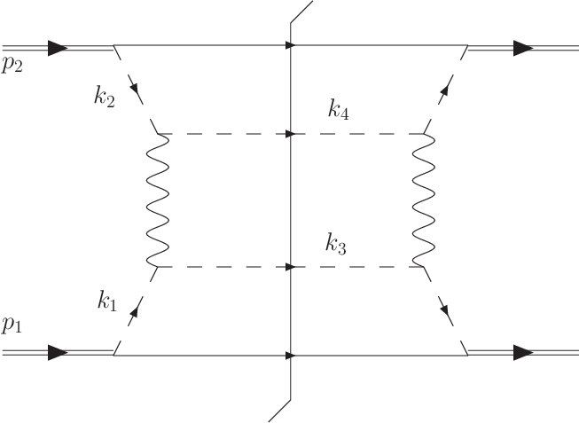
The basic graph contributing to hadro-production of high- hadrons, with no extra gluon attachments, is shown in Fig. 1. Because of the trivial color structure of the hard part, and the simplicity of our model of quarks and spectators, there is only one subprocess and one color flow. So a generalized TMD-factorization formula corresponding to Eq. (3) can only involve one term.
We work in the center-of-mass frame where the incoming hadron is initially moving with large rapidity in the forward plus direction with no transverse momentum, while is initially moving with large rapidity in the minus direction with no transverse momentum. Each hadron splits into an active “quark” which enters the hard subgraph, and a spectator “diquark” which enters the final state. The quarks interact in the hard part by exchanging a hard colorless vector boson , with momentum where is large, . Within the model, the final state high transverse momentum hadrons or jets are represented simply by on-shell final state quarks.
The polarization dependent differential cross section at zeroth order in is,
| (4) |
The factor of comes from tracing over the unit color triplet matrices in the upper and lower color loops in Fig. 1. We will use the approximation that the struck partons are collinear to the directions of their parent hadrons. So, and . The minus component of and the plus component of are small (order ) and can be neglected inside the hard part. We also define and , and is the usual Mandelstam variable for center-of-mass energy squared. The transverse spin vectors label the transverse spin for hadrons and are normalized such that the extreme values are . The subscript on indicates a trace over Dirac indices.
 |
 |
| (a) | (b) |
After evaluating the -functions, this cross section easily factorizes:
| (5) |
where the hard part is,
| (6) |
The remaining factors in braces in Eq. (5) are what is expected from the zeroth order expansion of the standard operator definition of a TMD PDF. For hadron , for example, the zeroth order TMD PDF is
| (7) |
and similarly for hadron . Note that is not kinematically independent of : . Also, and . To keep the expression simple, we have written Eq. (6) in terms of exact parton momenta, ,,,, though we remark that in the correct final formula these should be replaced by the approximate on-shell parton momenta appropriate for a hard subgraph 11 1 Because in Eq. (4) there is an integration over all , one generally must be careful in treating the region where the goes to zero in the hard part. For this paper, we are specifically interested in the collinear region where is small, so we will assume that any contribution from close to zero is removed by a cutoff on large ..
When treating higher order graphs, we will always work in Feynman gauge, where the contour deformations needed in a derivation of factorization are most straightforward. For factorization to work, it must be possible to identify any uncanceled collinear or soft singularities as contributions to non-perturbative correlation functions. Some of these singularities correspond to Wilson line contributions, and are therefore essential for maintaining gauge invariance.
Before continuing we should mention that there are a number of general complications involved in deriving TMD-factorization that will not be addressed here because they are not directly related to the main reasons that generalized TMD-factorization fails. The most naive definitions of TMD correlation functions include extra divergences that need to be removed by appropriate redefinitions (see Ref. [22] and references therein for an overview of issues related to the precise definition of a TMD PDF). One particular complication is that the Wilson lines in these definitions cannot be exactly light-like without containing extra “light-cone” divergences which correspond to partons moving with large rapidity opposite to the direction of their parent hadrons. Proposed solutions involve either tilting the Wilson line away from the exactly light-like direction [4], or dividing out by extra gauge invariant factors [6, 23, 24, 25]. Furthermore, an exactly correct factorization formula requires a soft factor to account for gluons with all components small. The other parton correlation functions tend to overlap in the soft region, and a fully correct definition of a TMD PDF requires extra factors to remove the overlap.
There has been much significant recent work devoted to finding a fully consistent definition of the TMD PDF. However, our main concern in this paper is only with the general color structure of the Wilson lines inside the matrix elements for the external hadrons. Therefore, for our purposes it will be sufficient to continue to treat the direction of the main Wilson lines in the TMD PDFs as being light-like, and we will not address the role of a soft factor or the overlap of regions. Finally, we will restrict consideration to the limit of very large relative transverse momentum (large-) where one expects standard pQCD methods to be most appropriate, and we do not consider the possibility of recovering a type of TMD-factorization appropriate in the small- limit [26].
Having discussed the basic graph in Fig. 1, the next step is to consider graphs dressed with extra gluons. The graphs which can contribute to the Wilson line insertions are those in which extra, nearly on-shell gluons connect different subgraphs — for example, graphs with gluons connecting the -collinear lines to the outgoing struck quark lines or to the -collinear lines. Normally, one expects the sum of such graphs to contribute to the Wilson line in the TMD PDF for , after application of a Ward identity. The primary issue is that the approximations that normally allow Ward identities to be applied are only valid after certain contour deformations on the extra momentum integrals. Namely, to apply a Ward identity, it must be possible to approximate an extra gluon by a longitudinally polarized one with a large component of longitudinal momentum. Then the extra gluon momentum can be contracted with the hard scattering matrix element and a Ward identity argument can be applied directly. However, when virtual gluons attach to a spectator line, they give contributions from the “Glauber” region, meaning that if is the momentum of an extra gluon, then and are both much smaller than . In the Glauber region, the approximations needed for the Ward identity are not valid. For factorization to work, it must be possible to first deform the contour out of the Glauber region (see, for example, Refs. [6]). Alternatively, factorization could be recovered if there is a cancellation between graphs, as in the standard proofs of integrated (collinear) factorization. The basic problem with TMD-factorization found in previous work [11, 12, 15, 17, 18] is that the necessary contour deformations needed to treat the Glauber region are inconsistent with a direct application of the standard Ward identity arguments. Namely, they are in different directions for different graphs depending on whether the interaction is in the initial or final state.
So, we will only consider graphs that can yield contributions from the Glauber region. Since real gluons can never be in the Glauber region, we will only consider graphs with virtual gluons. Also, as long as no restrictions are placed on the target remnant momenta, graphs with spectator-spectator interactions cancel [5] in the integration over final states 22 2 In a general proof of factorization, one may need to worry about cancellations in the “supersoft” region, , since we are now using a massless theory, in contrast to Ref. [17]. In this paper, we are concerned mainly with gluons with so these issues do not affect our argument.. Similar cancellations occur between different cuts of the same graph for active-spectator interactions after parton transverse momentum is integrated over, and are needed in the standard proofs of collinear factorization [5]. A counter-proof of TMD-factorizaton therefore needs to show that such cancellations generally fail when transverse parton momentum is explicitly taken into account. A specific example of such a non-cancellation was given in Ref. [18] and will be reviewed in Sect. IV. In graphs with attachments between active quarks, there are not enough Dirac -matrices to give spin dependence to the TMD PDFs. Such graphs will therefore not affect our discussion of single and double spin asymmetries at lowest non-vanishing order. Furthermore, graphs with a scalar-scalar-gluon-gluon vertex do not give leading power contributions to eikonal factors.
We remark that, because the TMD factorization breaking effects are due to the Glauber region where all components of gluon momentum are small, the interactions responsible for breaking TMD factorization are associated with large distance scales.
In our specific model, a large number of graphs vanish simply because of the highly simple color structure involved. Examples are shown in Fig. 2. They vanish because their color factors include a trace around a color loop of a single generator, . (The on the denotes a trace over triplet color indices.)
Hence, the relevant types of graphs are represented by Figs. 3 through 8. If a generalized TMD-factorization formula is possible, then the sum over all such graphs must produce a factorized form like Eq. (3) with a Wilson line structure in the TMD PDF or FF for each hadron separately. We will consider each type of graph in the following sections.
 |
 |
| (a) | (b) |
 |
 |
| (c) | (d) |
 |
 |
| (a) | (b) |
 |
 |
| (c) | (d) |
III One Extra Gluon
We begin the investigation of diagrams by reviewing the steps for determining the contribution from a single extra gluon. As in Ref. [17], we focus on the calculation of an SSA. We start with graphs of the type shown in Fig. 3, where the extra gluon attaches on the side of the hard part nearest to its parent hadron. Any spin asymmetry disappears in the zeroth order cross section, Fig. 1 because there are too few Dirac matrices to produce a non-zero result in the traces with .
Consider, for example, Fig. 3(a). The arrow on the gluon line indicates that it is collinear to . By first deforming the integral out of the Glauber region to the -collinear region, one may replace the intermediate struck quark line of momentum by the eikonal factor
| (8) |
where . The sign on the is determined by the direction of the contour deformation. For the spin-dependent part, the attachment of the extra gluon at the spectator produces a factor at leading power equal to
| (9) |
When this expression is combined with the imaginary part of Eq. (8), the factors of and combine and a contribution to an SSA is obtained. The is the two-dimensional Levi-Civita symbol with .
If the extra gluon is on the other side of the cut as in Fig. 3(b), the eikonal factor is
| (10) |
The factor from the attachment at the spectator is,
| (11) |
When this is combined with the imaginary part of Eq. (10), the factors of and combine and a contribution to an SSA is again obtained. It is exactly equal to the one found in Fig. 3(a) as it must be since the graphs are related by Hermitian conjugation.
Analogous steps apply to Figs. 3(c,d). The different shadings on the arrows is to emphasize that they are radiated from rather than . Now, after a contour deformation can be made collinear to the minus direction, and a vector is used instead of . The eikonal factors are,
| (12) |
for Fig. 3(c) and
| (13) |
for Fig. 3(d).
In our calculation of the SSA, is unpolarized so there is no factor of coming from the attachment to the upper spectator. Therefore, it is only the real principal value contributions that are kept in Eqs. (12,13). Note that there can be no double Sivers effect at the level of one extra gluon because there must be at least one extra gluon from each of the hadrons for their PDFs to have spin dependence.
The s in Eqs. (8,10) combine with the s in Eq. (9,11) to produce an overall color factor equal to
| (14) |
Exactly the same color factor also arises when is collinear to as in Figs. 3(c,d).
The remaining type of single-gluon graphs are those in Fig. 4. For the lines collinear to the eikonal propagators are
| (15) |
from Fig. 4(a) and
| (16) |
from Fig. 4(b). The sum of these graphs gives a contribution equal to
| (17) |
If the color factor in Eq. (17) did not vanish, then it would contribute to an SSA when the factor of combines with the factor of in Eq. (9). The same result is obtained from the Hermitian conjugate graphs. In a totally unpolarized cross section, there would be no contribution from Eq. (17), regardless of the color factor, since it is imaginary.
A symmetric analysis applies if the extra gluon is instead radiated from hadron as in Figs. 4(c,d). In that case is replaced by and is replaced by . Since is unpolarized, it is the real parts of the eikonal factors that contribute. Thus, since the real parts cancel between graphs, the eikonal factors from Fig. 4(c,d) do not contribute to the unpolarized TMD PDF of hadron .
The uncanceled terms like Eq. (17) would ordinarily signal a breakdown of standard TMD-factorization because they are not consistent with the standard Wilson line structure in a TMD PDF. This is exactly what is observed for the Abelian gauge theory calculation in Ref. [17]. In our non-Abelian example, however, these single extra gluon contributions to a “factorization anomaly” are exactly zero because they happen to include the trivial color factor:
| (18) |
So, in our specific non-Abelian calculation, Eqs. (8, 10) are the only eikonal propagators that contribute to an SSA at the level of just one extra gluon.
The non-vanishing eikonal factors (coming from Figs. 3(a,b)) are exactly what is obtained from an order expansion of the Wilson lines in the standard definition of the TMD PDFs:
| (19) |
The standard Wilson line operator is inserted between the two scalar quark fields. The triplet color indices are shown explicitly to emphasize the flow of color. The full Wilson line insertion is,
| (20) |
where
| (21) |
with denoting a path-ordering operator. The superscript in Eq. (19) refers to the direction of the main leg of the Wilson line, starting from point . The extra gluon attachment in Fig. 3(a) on the left side of the cut contributes to while the extra gluon in Fig. 3(b) contributes to . To close the Wilson line and ensure that it is exactly gauge invariant, the path needs a transverse link at light-cone infinity [27],
| (22) |
where is a path in the transverse direction connecting the points, and . In a derivation of TMD-factorization in Feynman gauge, contributions to the link at infinity do not arise explicitly. (See, e.g., Refs. [3, 8, 22] and references therein for a review of the steps for resumming collinear gluon attachments and identifying the resulting gauge links.)
Note that the Wilson line insertion in the standard TMD PDF of Eq. (19) contracts the color indices of the quark fields, so has no leftover color indices — it is a real-valued function as is appropriate for a gauge invariant probability density.
Similar steps result in the single-gluon contribution to the Wilson line in the standard TMD PDF for when the extra gluon is radiated from the upper spectator as in Figs. 3(c,d). There the Wilson line insertion instead points in the direction :
| (23) |
In the Abelian case considered in Ref. [17], breaking of standard TMD-factorization was observed for an SSA because the factorization anomaly terms analogous to Eq. (17) did not vanish. There, the “color factor” was the Abelian charge for Abelian “gluons” rather than the non-Abelian color factor . That the anomalous terms vanish at the level of one extra gluon in our non-Abelian example is only due to the highly simple color structure in the particular hard process that we have considered. Generally, when color is exchanged in the hard part, standard TMD-factorization breaking will already appear at the level of one extra gluon. In our example, violations of standard TMD-factorization only appear at the level of two extra gluons or higher.
Schematically, the standard TMD-factorization formula suggested by the sum of one-extra-gluon graphs in Figs. 3(a-d) is
| (24) |
Here is the same hard factor that appeared at zeroth order in Sect. II. The “” on the equal sign is to emphasize that this formula is ultimately incorrect, as explained in Refs. [17, 18]. We will see this explicitly at the level two extra gluons in the next section.
IV Two Extra Gluons

 |
 |
| (a) | (b) |
 |
 |
| (c) | (d) |
 |
 |
| (a) | (b) |
In this section we review the steps for illustrating a violation of standard TMD-factorization at the level of two extra gluons radiated from one of the hadrons. The structure of the resulting TMD-factorization anomaly terms constrains the possible generalizations of TMD-factorization, as we will discuss more in Sect. V.
The simple color structure of the hard process strongly limits the number of non-vanishing graphs. All graphs in which the second gluon is internal to the hadron subgraph (e.g. Fig. 5) only give further contributions to a single gluon contribution in the standard Wilson lines in Eq. (24). The only non-vanishing graphs that give order contributions to a Wilson line operator are of the type shown in Figs. 6, 7, 8. All other graphs vanish because they include an overall color factor .
We will consider each type of graph in turn in the next few subsections. We will first identify the graphs that are consistent with the standard TMD-factorization formula Eq. (24). Next we will consider the graphs that contribute to a violation of standard TMD-factorization that were already discussed in Refs. [18]. The remaining graphs in Fig. 8 are ultimately responsible for breaking generalized factorization, so we will put off any further discussion of them until Sect. VI.
IV.1 Graphs Contributing to Standard Factorization
By repeating the steps of Sect. III, graphs of the type shown in Figs. 6 lead to the Wilson lines in Eqs. (19, 23) for the TMD PDFs of the standard TMD-factorization formula. The eikonal factors that arise from Figs. 6(a,b) correspond to keeping the order Wilson line contribution from each of the TMD PDFs individually. Figures 6(c,d) (and related graphs) correspond to keeping the order Wilson line contributions in one of the TMD PDFs, and the zeroth order from the other.
The graphs considered up to now exhaust the contributions obtained by expanding each of the Wilson lines in the standard TMD-factorization formula Eq. (24) up to order (in the Wilson line). Therefore, any remaining uncanceled contributions from the graphs of the type shown in Figs. 7, 8 violate the standard TMD-factorization formula.
IV.2 Violation of Standard TMD-Factorization
The graphs of the type shown in Fig. 7, where two gluons attach the spectator of one hadron to the opposite side of the hard subgraph, have been shown in Refs. [18, 20] to be non-vanishing in calculations of both the unpolarized cross section and an SSA for an Abelian gauge theory. These graphs, therefore, yield a violation of the standard TMD-factorization formula Eq. (24).
The contribution to an anomalous SSA requires an imaginary part from the extra eikonal factors. In Ref. [18] the imaginary part came from graphs with one gluon attaching near to the parent hadron and the other attaching near to the opposite hadron (e.g., Fig. 2(b)). These graphs vanish in our model because they again include a color factor .
The non-cancellation of the unpolarized factorization anomaly, however, remains. It arises from graphs with both extra gluons radiating from the same hadron and attaching at the side of the hard subgraph near to the opposite hadron, as in Fig. 7. To make the violation of standard TMD-factorization explicit, we will briefly review the steps of Ref. [18]. We are for the moment only concerned with the unpolarized cross section so we will temporarily simplify the model of Sect. II by making all the hadron and spectator fields scalars. We further simplify the calculation by assuming .
For the graphs with the extra gluons on opposite sides of the cut (Fig. 7(a) and related graphs), the factorization anomaly for the unpolarized cross section comes from replacing the extra off-shell quark propagators by their eikonal propagators. Including all ways of attaching and to the and lines, one finds the same result as in Ref. [18], but with the Abelian and charges replaced by the appropriate color factor:
| (25) |
For the graphs with both extra gluons coupling on the same side of the cut (Fig. 7(b) and related graphs)), the steps are similar. Again including all ways of attaching and at the upper part of the graph, one finds
| (26) |
The anomalous eikonal factor here is the same as in Eq. (25), apart from an overall minus-sign. However, the propagator denominators for graphs like Fig. 7(a) (both gluons on opposite sides of the cut) are different from the propagator denominators for graphs like Fig. 7(b) (gluons on the same side). For graphs with the extra gluons on opposite sides of the cut, one finds the following contribution to the TMD PDF of hadron :
| (27) |
This is the same result as in Ref. [18], except that the gluon is massless and there is a non-Abelian color factor multiplying the integral. Equation (26) allows for a similar calculation of the remaining contribution to the TMD PDF for hadron from the graphs with the extra gluons on the same side of the cut:
| (28) |
The mismatch in denominators between Eq. (27) and Eq. (28) means that the full contribution does not generally vanish point-by-point in . The sum of graphs like Fig. 7 therefore results in uncanceled terms that are not accounted for by the standard Wilson lines. Hence, the standard TMD-factorization formula Eq. (24) fails for unpolarized scattering.
Exactly analogous observations apply to the TMD PDF of the other hadron if the two extra gluons are radiated from the spectator in , collinear to the minus direction. In that case, the eikonal factors analogous to Eqs. (25, 26) will instead use a vector and the delta functions from the eikonal factors will be and 33 3 In earlier sections we neglected gluon exchanges between active quarks because they do not lead to spin dependence. In the unpolarized cross section, the complete result is obtained only after including interactions between active quarks. In the collinear regions they result in the same set of eikonal factors as in Eqs. (25, 26) and analogous Wilson line contributions. The key point is that the usual steps that normally would lead to a cancellation of the factorization anomaly between different cuts of the same graph in collinear factorization, fails in the transverse momentum dependent case.. So, both TMD PDFs yield factorization anomalies at the two-gluon level in the unpolarized cross section.
V Generalized TMD-factorization
From the factorization anomaly terms Eqs. (25, 26) one may determine what the modified gauge link structure must be for the TMD PDF of hadron in a generalized factorization formula [9, 12, 15]. In our example, the sequence of eikonal factors in the factorization anomaly terms of Eqs. (25,26), including the trace around a color loop, require a color-traced Wilson loop operator to be inserted into the definition, Eq. (19), of the TMD PDF for . Each of the eikonal factors in Eqs. (25,26) corresponds to an attachment to a leg of the Wilson loop. Therefore, the standard TMD PDF in Eq. (24) for should be replaced with,
| (29) |
This is the same as the standard TMD PDF definition in Eq. (19) apart from the insertion of the following color-traced Wilson loop operator:
| (30) |
The sequence of eikonal factors in Eqs. (25,26) correspond exactly to gluons attaching to the “” Wilson lines in Eq. (30). As before, the transverse links at infinity do not contribute to leading power in Feynman gauge. The color trace corresponds to the trace over the color loop in the upper part of the graphs in Fig. 7 and is what is needed to get the factor of in Eqs. (25,26). Hence, the terms that violate standard factorization arise from expanding the operator in Eq. (29) up to order (see also Ref. [20]).
An exactly analogous TMD PDF is obtained for hadron when both extra gluons are radiated from in the collinear minus direction and attach to the lower half of the graph. The main legs of the Wilson loop in the TMD PDF for point in the direction of a vector :
| (31) |
Thus, the factorization anomaly terms from Sect. IV.2 specify the type of new Wilson line insertions that are needed if generalized TMD-factorization is to hold. The generalized TMD-factorization formula is:
| (32) |
Again, is the same hard factor that appeared at zeroth order in Sect. II. The only difference from Eq. (24) comes from the insertions in the TMD PDFs, indicated by the superscripts on the individual TMD PDFs in Eq. (32). We have again included a “” over the equal sign to indicate that even this formula will ultimately fail when the remaining graphs are considered.
Equation (32), with the TMD PDFs defined as in Eq. (29), follows the method proposed in [9, 12, 15], and is the most natural generalization of TMD-factorization. For the purpose of our counter-argument to generalized TMD-factorization, the crucial point is that the new Wilson line insertion Eq. (30) involves a trace over color. If we instead tried contracting the color indices of the new Wilson lines with the quark fields at points and , then we would obtain the wrong color factor for the anomalous contribution in Eqs. (25,26). An even more serious problem would be that the generalized TMD-factorization formula would produce spurious terms at the one-gluon level, already treated in Sect. III. Namely, single-gluon attachments to the extra legs of the Wilson line would introduce factorization anomaly contributions analogous to Eq. (17), but with different non-vanishing color factors, contradicting the analysis from Sect. III which found no violation of standard TMD-factorization at order in the expansion of the Wilson lines (polarized or unpolarized). Thus, consistency between the order- and order- contributions to the Wilson lines requires that the new Wilson line structures include the trace over color as in Eq. (30).
Other possible redefinitions of the TMD PDFs are unrelated to the color structure of the Wilson lines in the main correlation functions. These include the modifications mentioned in Sect. II, such as tilting the direction of the Wilson line slightly away from the light-like direction. Thus, accounting for all contributions up to order , in the Wilson line, and requiring consistency between different orders in , strongly constrains the possibilities for a generalization of TMD-factorization.
 |
 |
| (a) | (b) |
The order- contribution from a Wilson loop in Eq. (32) is zero simply because, with one gluon attaching to the Wilson loop, the color trace in the definition of the Wilson line operator Eq. (30) involves only one color generator . So,
| (33) |
Therefore, there is no disagreement between Eq. (32) and standard factorization, Eq. (24), from graphs with only one extra gluon. To find a disagreement between the standard and generalized TMD-factorization formulas (Eqs. (24) and (32)), at least two gluons need to be collinear to one of the hadrons as in Sect. IV.2.
VI Breakdown of Generalized TMD-Factorization
We will now directly illustrate a breakdown of the generalized TMD-factorization formula Eq. (32) by calculating the anomalous two-gluon contribution to a double Sivers effect from the graphs in Fig. 8. First, let us summarize the situation so far:
- •
- •
- •
The two-gluon factorization anomaly terms found in Sect. IV.2 specify which modifications of the Wilson lines in the TMD PDFs are needed if a form of factorization is to be recovered. It is found that the modified TMD PDFs must each contain an extra color-traced Wilson loop, as in Eq. (29). This result also follows from the same steps for finding general Wilson line structures from low order graphs as discussed in Ref. [12].
- •
Because of Eq. (33), the generalized TMD-factorizaton formula Eq. (32) cannot include any other two-gluon contributions to Wilson lines. In particular, there can be no contribution that corresponds to graphs like Fig. 8, where one gluon is radiated collinear to each hadron simultaneously. These graphs would correspond to separate order- contributions from the Wilson lines in separate TMD PDFs. If they are non-zero, then they contribute to a violation of both standard TMD-factorization in Eq. (24) and the generalized TMD factorization formula in Eq. (32). To incorporate such a contribution, one would have to modify the Wilson line in each TMD PDF such that it includes a single-gluon contribution to a factorization anomaly. But this would contradict Sect. III where it was shown that there is no violation of standard factorization with just one gluon. Hence, contributions from graphs like Fig. 8 cannot be consistently incorporated into a generalization of factorization simply by modifying Wilson lines in separate correlation functions. If they give a non-vanishing contribution, then there is a clear violation of generalized TMD-factorization.
We will therefore prove that generalized TMD-factorization, Eq. (32), is violated by showing that the sum of graphs of the type illustrated in Fig. 8 give a non-vanishing contribution to a DSA.
First, we note that all graphs of the type shown in Fig. 8 include the non-zero color factor
| (34) |
Next, we must ensure that there is no cancellation between graphs.
VI.1 Same Side of the Cut
In the sum of graphs like Fig. 8(a), where both gluons are on the same side of the cut, the eikonal factors give a total contribution equal to
| (35) |
Since spin dependence is needed in both and for a DSA, then there are also two factors corresponding to Eq. (9) (but with one corresponding to a spectator attachment). Taking into account both of the resulting factors of gives an overall factor of . Combined with Eq. (35), the relevant factor from extra collinear gluons is then . The same result is obtained from the Hermitian conjugate graphs.
VI.2 Opposite Side of Cut
The sum of graphs with one extra gluon on each side of the cut, as in Fig. 8(b), works in much the same way. The eikonal factors give
| (36) |
For a DSA, there is a factor of from a factor analogous to Eq. (9) for the -spectator attachment of the gluon on the left side of the cut and a factor of from a factor analogous to Eq. (11) (but for a gluon attaching at the -spectator) on the right side of the cut, giving an overall factor of . So, combined with Eq. (36) the relevant factor from extra gluon attachments is again .
VI.3 Together
Summing all graphs of the type shown in Fig. 8, therefore, results in just a single integral. To check it explicitly, one can use Eqs. (36) (extracting the overall factor of that comes with the two spectator attachments) to explicitly calculate the contribution from graphs with gluons on opposite sides of the cut:
| (37) |
Here we have dropped the irrelevant factors of , , and which appeared in Eq. (4). We have also dropped the and dependence inside the factor in braces. This is permitted because the -functions will set and to zero, and because the other components yield power suppressed corrections. The -functions can be used to evaluate the ,,, , , and integrals, and the and integrals can be evaluated by contour integration. The result is
| (38) |
The factor is now the hard part in Eq. (6). The symbol “” in the denominators refers to terms that involve only , and masses. For graphs with both gluons on the same side of the cut, exactly the same result (with the same overall sign) is obtained by using Eq. (35) and taking into account the overall factor of that comes from the two spectator attachments. There are, again, identical results coming from the Hermitian conjugate graphs.
The integral in Eq. (38) is not generally zero as can be checked by considering a fixed . However, there is no corresponding factorization anomaly term contained in an expansion of Eq. (32) up to order in the Wilson lines. The modified Wilson lines in the TMD PDFs of the generalized TMD-factorization formula are specified by the factorization anomaly terms that arise when gluons are radiated from just one hadron at a time, as in Sect. IV. However, the resulting generalized TMD-factorization formula is in contradiction with graphs like Fig. 8, where there are simultaneously gluons radiated from and . Thus, generalized TMD-factorization breaks down at the two-gluon level.
Indeed, at up to two gluons, the generalized TMD-factorization formula Eq. (32) gives no contribution to a DSA beyond what is predicted by the standard TMD-factorization formula Eq. (24). The only factorization anomaly contribution from Eq. (32) is to the unpolarized cross section, and arises from graphs with both extra gluons radiated from the same hadron. There must be at least one gluon coming from each hadron at the same time to have spin dependence in both hadrons simultaneously. So, the only contribution to a double Sivers effect that violates standard TMD-factorization is from the sum of graphs in Fig. 8, and these are not accounted for in Eq. (32). To recover the factorization anomaly in the DSA, one would have to somehow allow each TMD PDF to have a non-vanishing factorization anomaly contribution at the level of one extra gluon. This, however, would contradict the single-extra-gluon treatment of the SSA in Sect. III. Therefore, a TMD-factorization formula cannot be recovered by simply modifying the Wilson lines in each TMD PDF separately. We have thus illustrated a specific example of a violation of generalized TMD-factorization.


One can interpret the breakdown of generalized TMD-factorization visually by imagining the flow of color in the factorized expression, Eq. (32), as compared to the original unfactorized graph. The graph in Fig. 8b, for example, must correspond to the product of two single-gluon contributions to the Wilson lines in Eq. (32), if that formula is correct. The resulting color structure can be visualized as in Fig. 9. The narrow double lines represent the Wilson lines in each TMD PDF. The box shaped Wilson lines represent the extra color-traced Wilson loops in Eq. (32). The color trace over each of the Wilson loops means that only a color singlet gluon can be exchanged between a Wilson loop and a spectator at the single-gluon level, as illustrated by the factors representing the TMD PDFs in Fig. 9. Therefore, these contributions to the TMD PDFs must vanish. By contrast, in the original unfactorized graph, the interlaced color flow of the two gluons means there is no problem with exchanging non-singlet color, as illustrated by the color flow diagram in Fig. 10. This corresponds to the non-zero color factor in Eq. (34).
VII Discussion and Conclusion
We have shown that a generalized TMD-factorization formula like Eq. (3)/Eq. (32) does not in general exist for back-to-back hadro-production of high- hadrons due to the non-trivial interplay of gluons that are collinear to both hadron directions. The failure of generalized TMD-factorization calls into question results that use it as a starting assumption. This includes calculations of weighted cross sections which retain a memory of the non-universality of the TMD PDFs.
It is interesting to note that the same complications do not seem to arise if the gauge field is Abelian. In that case, the Abelian “color factors” can be identified with coupling constants, such as in the model from Ref. [17]. Then the contribution to a DSA from graphs like Fig. 8 is indeed just a product of single gluon contributions to Wilson loops from separate correlation functions (which are non-zero in the Abelian case). Therefore, there is no obvious contradiction with generalized TMD-factorization for the Abelian case, at least at the level of graphs discussed here. While a full proof of generalized TMD-factorization for the Abelian gauge theory does not yet exist, the breakdown of generalized TMD-factorization that we have found is a specific consequence of the non-Abelian nature of QCD.
It is worth stressing that the failure of generalized TMD-factorization occurs in a regime where factorization would ordinarily be expected to apply; namely for hard processes with large-. Moreover, it should not be thought that the breakdown of generalized TMD-factorization is specific to a DSA or SSA. We have calculated for a DSA with color singlet boson exchange for the hard part in order to maximize the simplicity of the argument, but the reasons for the breakdown are quite general. The counter-example we have provided in this paper is sufficient to show that a general proof does not exist. That is, it is not possible to consistently define TMD PDFs for each hadron separately, even if we allow for process dependence in the Wilson line structures. To encounter the same complications with generalized TMD-factorization in an unpolarized cross section, one needs the type of non-cancellation that was found in Sect. IV.2 (which comes from having two gluons collinear to one hadron), but with at least one more gluon collinear to the opposite hadron. An example of the type of graph which can produce a violation of generalized TMD-factorization in the unpolarized cross section is shown in Fig. 11.
Furthermore, the contribution from extra gluon attachments (which lead to factorization breaking) should not be thought of as negligible higher order corrections. They correspond to soft and collinear divergences in higher order hard scattering calculations. In real QCD, they are non-perturbative gluons in the strong coupling regime. For the perturbation series to have sensible convergence properties, it must be possible to rearrange terms such that the extra soft and collinear gluons are resummed to all orders into TMD PDFs. We also remark that, at the level of many extra gluons, there are more graphs with gluons collinear to both hadrons simultaneously (which led to a breakdown of generalized TMD-factorization) than graphs with gluons radiated from one hadron only.
While the observation of generalized TMD factorization breaking leads to frustrating practical difficulties in cross section calculations, it should not necessarily be regarded as a purely negative result. The question of whether transverse momentum effects can be meaningfully associated with parton transverse momentum in separate parton correlation functions for each hadron is intrinsically important in the search for an improved fundamental understanding of QCD dynamics in hard collisions. A counter-proof implies the existence of effects which challenge normal partonic intuition, and suggests new avenues of research. While naive factorization fails, the fact that the extra gluons eikonalize suggests that Wilson lines still may play a role. Insight might be gained, for example, from methods currently being applied to small- physics (e.g. [28, 29]). Another possibility is to model factorization breaking effects by directly calculating factorization breaking phase contributions in perturbation theory, but with explicit infrared and collinear cutoffs.
It is possible to understand the origin of the generalized TMD-factorization breakdown intuitively as arising from non-linear effects in the phases acquired by partons as they pass through the and fields of the colliding hadrons. If the overall phase were simply the product of the phases induced by the fields from hadron and the fields from hadron , then one could associate any process-dependent phases induced by the field in hadron with a modified Wilson line for the TMD PDF of and, likewise, any process-dependent phases induced by the field from could be associated with a modified Wilson line for the TMD PDF of . However, in the non-Abelian theory the role of the gluons in is affected by the presence of the gluons from and visa-versa. A direct example of this is Fig. 8/Eq. (38), where a single gluon exchanged between and the opposite-side struck quark gives a non-zero contribution, but only because there is simultaneously an gluon exchanged between and the other struck quark. This means that one cannot address the role of phases induced by the and fields independently, but instead must deal with them simultaneously. The result is a kind of nonperturbative correlation which cannot be identified as arising strictly from gluons coming from either hadron independently, but only from the combination.
Acknowledgments
We would especially like to thank D. Boer and C. Mantz for useful discussions. One of us (T. Rogers) would like to thank J. Collins for helpful discussions. Support was provided by the research program of the “Stichting voor Fundamenteel Onderzoek der Materie (FOM)”, which is financially supported by the “Nederlandse Organisatie voor Wetenschappelijk Onderzoek (NWO)”. All figures were made using Jaxodraw [30].
References
- [1] D. Boer, P. J. Mulders and C. Pisano, arXiv:0909.4652 [hep-ph].
- [2] Z. Lu and I. Schmidt, Phys. Rev. D 78, 034041 (2008) [arXiv:0805.4006 [hep-ph]].
- [3] J. C. Collins, D. E. Soper and G. Sterman, Adv. Ser. Direct. High Energy Phys. 5, 1 (1988) [arXiv:hep-ph/0409313].
- [4] J. C. Collins and D. E. Soper, Nucl. Phys. B 194, 445 (1982).
- [5]
J. C. Collins, D. E. Soper and G. Sterman,
Nucl. Phys. B 261, 104 (1985).
J. C. Collins, D. E. Soper and G. Sterman, Nucl. Phys. B 308, 833 (1988).
G. T. Bodwin, Phys. Rev. D 31, 2616 (1985) [Erratum-ibid. D 34, 3932 (1986)]. - [6] J. C. Collins and A. Metz, Phys. Rev. Lett. 93, 252001 (2004) [arXiv:hep-ph/0408249].
- [7] J. C. Collins, Phys. Lett. B 536, 43 (2002) [arXiv:hep-ph/0204004].
- [8] D. Boer, P. J. Mulders and F. Pijlman, Nucl. Phys. B 667, 201 (2003) [arXiv:hep-ph/0303034].
- [9] C. J. Bomhof, P. J. Mulders and F. Pijlman, Phys. Lett. B 596, 277 (2004) [arXiv:hep-ph/0406099].
- [10] S. M. Aybat and G. Sterman, Phys. Lett. B 671, 46 (2009) [arXiv:0811.0246 [hep-ph]].
- [11] A. Bacchetta, C. J. Bomhof, P. J. Mulders and F. Pijlman, Phys. Rev. D 72, 034030 (2005) [arXiv:hep-ph/0505268].
- [12] C. J. Bomhof, P. J. Mulders and F. Pijlman, Eur. Phys. J. C 47, 147 (2006) [arXiv:hep-ph/0601171].
- [13] A. Bacchetta, C. Bomhof, U. D’Alesio, P. J. Mulders and F. Murgia, Phys. Rev. Lett. 99, 212002 (2007) [arXiv:hep-ph/0703153].
- [14] C. J. Bomhof, P. J. Mulders, W. Vogelsang and F. Yuan, Phys. Rev. D 75, 074019 (2007) [arXiv:hep-ph/0701277].
- [15] C. J. Bomhof and P. J. Mulders, Nucl. Phys. B 795, 409 (2008) [arXiv:0709.1390 [hep-ph]].
- [16] D. Boer, P. J. Mulders and C. Pisano, Phys. Lett. B 660, 360 (2008) [arXiv:0712.0777 [hep-ph]].
- [17] J.C. Collins and J.W. Qiu, Phys. Rev. D 75, 114014 (2007).
- [18] J. Collins, arXiv:0708.4410 [hep-ph].
- [19]
J. W. Qiu, W. Vogelsang and F. Yuan,
Phys. Lett. B 650, 373 (2007)
[arXiv:0704.1153 [hep-ph]].
J. W. Qiu, W. Vogelsang and F. Yuan, Phys. Rev. D 76, 074029 (2007) [arXiv:0706.1196 [hep-ph]]. - [20] W. Vogelsang and F. Yuan, Phys. Rev. D 76, 094013 (2007) [arXiv:0708.4398 [hep-ph]].
- [21] S. J. Brodsky, D. S. Hwang and I. Schmidt, Phys. Lett. B 530, 99 (2002) [arXiv:hep-ph/0201296].
- [22] J. Collins, PoS LC2008, 028 (2008) [arXiv:0808.2665 [hep-ph]].
- [23] F. Hautmann, Phys. Lett. B 655, 26 (2007) [arXiv:hep-ph/0702196].
- [24]
J. C. Collins and F. Hautmann,
JHEP 0103, 016 (2001)
[arXiv:hep-ph/0009286].
J. C. Collins and F. Hautmann, Phys. Lett. B 472, 129 (2000) [arXiv:hep-ph/9908467]. - [25] J. C. Collins, Acta Phys. Polon. B 34 (2003) 3103 [arXiv:hep-ph/0304122].
- [26] C. p. Chang and H. n. Li, arXiv:0904.4150 [hep-ph].
- [27] A. V. Belitsky, X. Ji and F. Yuan, Nucl. Phys. B 656, 165 (2003) [arXiv:hep-ph/0208038].
- [28]
F. Gelis, T. Lappi and R. Venugopalan,
Phys. Rev. D 78, 054019 (2008)
H. Fujii, F. Gelis and R. Venugopalan, Nucl. Phys. A 774, 793 (2006) [arXiv:hep-ph/0510053]. - [29] I. Balitsky, arXiv:hep-ph/0101042.
- [30]
D. Binosi and L. Theussl,
Comput. Phys. Commun. 161, 76 (2004)
[arXiv:hep-ph/0309015].
D. Binosi, J. Collins, C. Kaufhold and L. Theussl, arXiv:0811.4113 [hep-ph].