Measurement of the CKM angle $\gamma$ ($\phi_{3}$) using $B\to DK$ decays

In the method proposed by Gronau, London and Wyler (GLW) [9] the $D$ meson is reconstructed to $CP$ eigenstate final states $f_{CP\pm}$, such as $K^{+}K^{-}$ ($CP=+1$) or $K^{0}_{S}\pi^{0}$ ($CP=-1$). Therefore $A_{f}/A_{\bar{f}}=1$, $\delta_{D}=0,\pi$ for $CP=1,-1$, and Eq. 2 becomes

Equation 3 and its $CP$-conjugate are used to define four observables which depend on the physical parameters $\gamma$, $\delta_{B}$ and $r_{B}$:

where $\Gamma(B^{-}\to D^{0}_{CP\pm}K^{-})\equiv\Gamma(B^{-}\rightarrow[f_{CP\pm}]_{D}K^{-})/BF(D^{0}\to f_{CP\pm})$ and $\Gamma(B^{-}\to D^{0}K^{-})\equiv A_{c}^{2}\simeq\Gamma(B^{-}\to[K^{-}\pi^{+}]_{D}K^{-})/BF(D^{0}\to K^{-}\pi^{+})$. $A_{CP\pm}$ and $R_{CP\pm}$ are bound by the relation $R_{CP+}A_{CP+}+R_{CP-}A_{CP-}=0$.

Both BaBar and Belle have reconstructed $B^{-}\to D^{0}K^{-}$ and $B^{-}\to D^{*0}K^{-}$ decays with $D^{*0}\to D^{0}\pi^{0}$. BaBar has also selected the mode $D^{*0}\to D^{0}\gamma$ and the decay $B^{-}\to D^{0}K^{*-}$ with $K^{*-}\to K_{S}^{0}\pi^{-}$. $D^{0}$ mesons have been reconstructed in $CP$-even ($K^{+}K^{-}$ and $\pi^{+}\pi^{-}$) and $CP$-odd ($K_{S}^{0}\pi^{0}$, $K_{S}^{0}\phi$ and $K_{S}^{0}\omega$) eigenstates. Recently also CDF has measured $B^{-}\to D^{0}K^{-}$ with $D^{0}\to K^{+}K^{-}$ and $\pi^{+}\pi^{-}$. The data samples used by BaBar and Belle consist of $382$ and $275$ million $B\bar{B}$ pairs, respectively, while CDF has used 1.0 fb^-1 of data. The results are summarized in Table 1.

Due to the discrete 8-fold ambiguity in the extraction of $\gamma$ from $R_{CP\pm}$ and $A_{CP\pm}$, and the still large uncertainty on $r_{B}$, the GLW measurements have a poor constraining power on $\gamma$ when they are considered alone. However, they generally improve the knowledge of $r_{B}$, $\gamma$ and $\delta_{B}$ when combined with the results of the Dalitz method discussed in Sec. 2.3. This aspect is further discussed in Sec. 3.

In the method proposed by Atwood, Dunietz and Soni (ADS) [15] the $D$ meson is reconstructed in doubly Cabibbo-suppressed (DCS) states. We consider $D^{0}\to K^{+}\pi^{-}$ as an example in the following discussion. The decay rate of the process $B^{-}\to[K^{+}\pi^{-}]_{D}K^{-}$ is the result of the interference between $B^{-}\to D^{0}K^{-}$ followed by the DCS $D^{0}\to K^{+}\pi^{-}$, and the suppressed $B^{-}\to\bar{D}^{0}K^{-}$ followed by the Cabibbo-allowed $\bar{D}^{0}\to K^{+}\pi^{-}$. From Eq. 2 we find

where both $r_{D}=A_{f}/A_{\bar{f}}=|A(D^{0}\rightarrow K^{+}\pi^{-})/A(D^{0}\rightarrow K^{-}\pi^{+})|$ and the strong phase difference $\delta_{D}$ are measured independently [2, 16]. Defining $R_{ADS}$ and $A_{ADS}$ as

it follows

Since $r_{D}(K\pi)=(5.78\pm 0.08)\%$ [17] and $r_{B}$ is expected to be around 10%, the interference effect can be quite large. Similar relations, with small modifications, are derived for $B^{-}\to D^{*0}K^{-}$ and $B^{-}\to D^{0}K^{*-}$ decays (see [6] and refs. in Table 2) and for multi-body $D^{0}$ final states [18, 19]. Both BaBar and Belle have reconstructed the decay $B^{-}\to D^{0}K^{-}$ followed by $D^{0}\to K^{+}\pi^{-}$ on datasets of 467 and 657 million $B\bar{B}$ pairs, respectively. BaBar has also selected $B^{-}\to D^{*0}K^{-}$ with $D^{*0}\to D^{0}\pi^{0}$ and $D^{*0}\to D^{0}\gamma$ ($467\times 10^{6}\,B\bar{B}$), and $B^{-}\to D^{0}K^{*-}$ with $K^{*-}\to K^{0}_{S}\pi^{-}$ ($379\times 10^{6}\,B\bar{B}$). On a dataset of 465 million $B\bar{B}$ pairs BaBar has performed the first measurement of flavor-tagged decays $B^{0}\to D^{0}K^{*0}$ with $K^{*0}\to K^{+}\pi^{-}$, selected in the $D^{0}$ final states $K^{+}\pi^{-}$, $K^{+}\pi^{-}\pi^{0}$ and $K^{+}\pi^{-}\pi^{-}\pi^{+}$. The results are summarized in Table 2. Due to the smallness of the involved branching fractions no evidence of signal has been observed so far and the null measurements have been used to set upper limits on $r_{B}$. The strongest hint of signal has been reported by BaBar with a statistical significance of $2.6\sigma$ for $B^{\mp}\to D^{0}[K^{\pm}\pi^{\mp}]K^{\mp}$. Even when a signal is observed the constraining power on $\gamma$ of the ADS method is weak when it is used alone, but it becomes significant when the ADS information is combined with the other methods. This aspect is discussed in Sec. 3.

If $D^{0}$ decays to a 3-body final state such as $D\to K^{0}_{S}\pi^{+}\pi^{-}$, the decay amplitudes of $D^{0}$ and $\bar{D}^{0}$ can be written as $A_{f}e^{i\delta_{f}}=f(m_{-}^{2},m_{+}^{2})$ and $A_{\bar{f}}e^{i\delta_{\bar{f}}}=f(m_{+}^{2},m_{-}^{2})$, where $m_{-}^{2}$ and $m_{+}^{2}$ are the squared masses of the $K^{0}_{S}\pi^{-}$ and $K^{0}_{S}\pi^{+}$ combinations. The rate in Eq. 2 becomes

where $\delta_{D}(m_{\mp}^{2},m_{\pm}^{2})$ is the strong phase difference between $f(m_{\pm}^{2},m_{\mp}^{2})$ and $f(m_{\mp}^{2},m_{\pm}^{2})$. The amplitudes $f(m_{\pm}^{2},m_{\mp}^{2})$ are measured through a Dalitz plot analysis on a large sample of flavor-tagged $D^{0}$ decays. Therefore, the $B^{\pm}$ yields in Eq. 11 only depend on the unknowns $\gamma$, $\delta_{B}$ and $r_{B}$. The great advantage of this method [23] is that the relation between the signal yields and the physics parameters varies over the Dalitz plot, making possible the extraction of $\gamma$ with only a 2-fold ambiguity ($\gamma\to\gamma+180^{\circ}$). Furthermore, the $D^{0}\to K^{0}_{S}\pi^{+}\pi^{-}$ branching fractions is relatively large ($\sim 3\%$). Since the direct extraction of $r_{B}$, $\delta_{B}$ and $\gamma$ through a maximum likelihood fit (MLF) using Eq. 11 overestimates $r_{B}$ and underestimates the statistical error of $\gamma$ and $\delta_{B}$, it is convenient to express Eq. 11 in terms of the cartesian coordinates $x_{\pm}={\rm Re}[r_{B}e^{i(\delta_{B}\pm\gamma)}]$, $y_{\pm}={\rm Im}[r_{B}e^{i(\delta_{B}\pm\gamma)}]$,

where the notation was simplified using $f_{\pm}=f(m_{\pm}^{2},m_{\mp}^{2})$. The extraction of $x_{\pm}$ and $y_{\pm}$ with a MLF using Eq. 12 is unbiased. The physics parameters $\gamma$, $r_{B}$ and $\delta_{B}$ are extracted from $x_{\pm}$ and $y_{\pm}$ with a frequentist statistical procedure.

BaBar has used this approach to measure the angle $\gamma$ with $B^{-}\rightarrow D^{0}K^{-}$, $D^{*0}K^{-}$ ($D^{*0}\to D^{0}\pi^{0}$ and $D^{0}\gamma$) and $D^{0}K^{*-}$ ($K^{*-}\to K^{0}_{S}\pi^{-}$), with $D^{0}\rightarrow K^{0}_{s}\pi^{+}\pi^{-}$ and $K^{0}_{S}K^{+}K^{-}$ using a sample of 386 million $B\bar{B}$ pairs[24]. Belle has selected $B^{-}\to D^{(*)0}K^{-}$ decays ($D^{*0}\to D^{0}\pi^{0}$ and $D^{0}\gamma$) with $D^{0}\to K^{0}_{S}\pi^{+}\pi^{-}$ on a sample of 657 million $B\bar{B}$ pairs [25]. The $D^{0}\to K^{0}_{S}\pi^{+}\pi^{-}$ and $D^{0}\to K^{0}_{S}K^{+}K^{-}$ decay amplitudes are determined with Dalitz plot analyses of large and very pure samples of $D^{0}$ mesons from $D^{*+}\to D^{0}\pi^{+}$ decays produced in $e^{+}e^{-}\to c\bar{c}$ events. The amplitudes are described using an isobar model, consisting of a coherent sum of two-body amplitudes (parameterized using relativistic Breit-Wigner) plus a “nonresonant” term. BaBar has described the $\pi\pi$ and $K\pi$ S-wave amplitudes in $D^{0}\to K^{0}_{S}\pi^{+}\pi^{-}$ using a $K$-matrix formalism (see [24] for a detailed discussion).

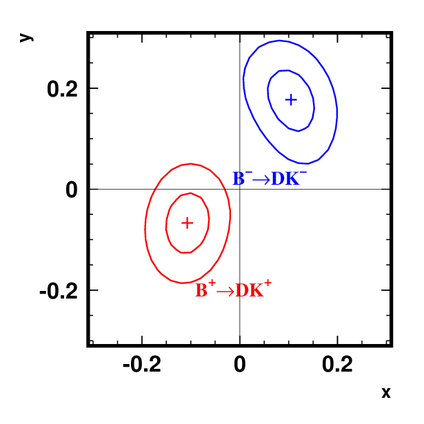
The results for $x_{\pm}$ and $y_{\pm}$ are reported in Table 3. From the $(x_{\pm},y_{\pm})$ confidence regions both BaBar and Belle determine the 1$\sigma$ confidence intervals of $\gamma$, $\delta_{B}$ and $r_{B}$ using a frequentist procedure. BaBar finds $\gamma=(76\pm 22\pm 5\pm 5)^{\circ}$ and Belle $\gamma=(76^{+12}_{-13}\pm 4\pm 9)^{\circ}$ ($B^{\pm}\to D^{(*)}K^{\pm}$), where the solution closest to the SM average has been quoted. All results are reported in Table 4. Figure 3 shows the $(x_{\pm},y_{\pm})$ contours for $B\to D^{0}K$ as measured by Belle (top-left) and BaBar (bottom-left), the projections of confidence regions onto the $(\gamma,r_{B})$ and $(\gamma,\delta_{B})$ plane obtained by Belle, and the confidence-level as a function of $r_{B}$ and $\gamma$ found by BaBar. The combined $B\to D^{(*)0}K^{(*)}$ measurements of BaBar and Belle correspond to 3.0$\sigma$ and 3.5$\sigma$ evidence of $CP$ violation, respectively.

It is interesting to ask why the statistical error measured by Belle is about twice smaller than what BaBar finds, despite the fact that the experimental observables $x_{\pm},y_{\pm}$ have similar uncertainties. The error on $\gamma$ scales roughly as $1/r_{B}$. Since Belle measurements have central values of $r_{B}$ between 1.5 and 3.5 times larger than BaBar values, though consistent within the errors, the resulting $\gamma$ uncertainty of Belle is smaller. The concept is illustrated in Fig. 4a. Fluctuactions of the $\gamma$ error due to the “$1/r_{B}$” effect are expected to decrease as the relative uncertainty on $r_{B}$ will become smaller.

At present the Dalitz method has the best sensitivity to $\gamma$. However, the uncertainty associated to the Dalitz model of the $D$ final state is already the dominant contribution to the systematic error and it may be difficult to reduce it greatly in the future. To bypass this limit a model-independent analysis is required [23]. At the price of a small loss of statistical power [29], the method is free of model-dependent assumptions on the $D$ decay and therefore it is a promising approach to follow at LHCb and at the next generation $B$-factories. It requires the use of entangled $\Psi(3770)\to D\bar{D}$ decays at tau-charm factories such as CLEO-c, BES-III or next generation Super Flavor factories [4]. It has been recently shown that using 818 pb^-1 of CLEO-c data an error on $\gamma$ of $\sim 2^{\circ}$ associated to the knowledge of the relative strong phase difference of $D^{0}\to K^{0}_{S}\pi^{+}\pi^{-}$ and $\bar{D}^{0}\to K^{0}_{S}\pi^{+}\pi^{-}$ can be obtained [30].

BaBar has applied the Dalitz method also to flavor-tagged $B^{0}\to D^{0}K^{*0}$ decays, with $K^{*0}\to K^{+}\pi^{-}$ and $D^{0}\to K^{0}_{S}\pi^{+}\pi^{-}$. On a dataset of 371 million $B\bar{B}$ pairs $39\pm 9$ signal candidates have been selected. Using the $D^{0}$ Dalitz plot model obtained in the charged $B$ analysis and imposing an external measurement of $r_{B}$, a loose constraint on $\gamma$ was set [31]. Self tagging $B^{0}\to D^{0}K^{*0}$ decays and time-dependent measurements of $B^{0}\to DK^{0}_{S}$ decays are expected to be powerful tools to measure $\gamma$ at LHCb and at the next generation $B$-factories, where their production will be abundant and the large interference ($r_{B}\sim 0.4$) can be fully exploited.

References

• [1] J. H. Christenson et al., Phys. Rev. Lett. 13, 138 (1964).
• [2] Particle Data Group, C. Amsler et al., Phys. Lett. B667, 1 (2008).
• [3] N. Cabibbo, Phys. Rev. Lett. 10, 531 (1963); M. Kobayashi and T. Maskawa, Prog. Theor. Phys. 49, 652 (1973).
• [4] See for example the SuperB Conceptual Design Report, arXiv:0709.0451.
• [5] See for example T. E. Browder et al., arXiv:0802.3201 and references therein.
• [6] A. Bondar and T. Gershon, Phys. Rev. D 70, 091503 (2004).
• [7] M. Gronau, Phys. Lett. B 557, 198 (2003).
• [8] T. Gershon, Phys. Rev. D 79, 051301 (2009); T. Gershon and M. Williams, Phys. Rev. D80, 092002 (2009); T. Gershon and A. Poluektov, arXiv:0910.5437.
• [9] M. Gronau and D. Wyler, Phys. Lett. B 265, 172 (1991); M. Gronau and D. London, Phys. Lett. B 253, 483 (1991).
• [10] BaBar Collaboration, B. Aubert et al., Phys. Rev. D 77, 111102 (2008).
• [11] Belle Collaboration, K. Abe et al., Phys. Rev. D 73, 051106 (2006).
• [12] CDF Collaboration, K. R. Gibson et al., arXiv:0809.4809.
• [13] BaBar Collaboration, B. Aubert et al., Phys. Rev. D 78, 092002 (2008).
• [14] BaBar Collaboration, B. Aubert et al., Phys. Rev. D 80, 092001 (2009).
• [15] D. Atwood, I. Dunietz and A Soni, Phys. Rev. Lett. 78, 3257 (1997).
• [16] CLEO Collaboration, D. M. Asner et al., Phys. Rev. D78, 012001 (2008).
• [17] E. Barberio et al., HFAG report, arXiv:0808:1297.
• [18] CLEO Collaboration, N. Lowrey et al., Phys. Rev. D80, 031105(R) (2009).
• [19] BaBar Collaboration, B. Aubert et al., Phys. Rev. D 76, 111101 (2007).
• [20] BaBar Collaboration, B. Aubert et al., Phys. Rev. D 72, 032004 (2005); new preliminary results presented at the Europhysics Conference On High Energy Physics 2009 (EPS2009).
• [21] Belle Collaboration, Y. Horii et al., Phys. Rev. D 78, 071901 (2008).
• [22] BaBar Collaboration, B. Aubert et al., Phys. Rev. D 80,031102(R) (2009).
• [23] A. Giri et al., Phys. Rev. D 68, 054018 (2003); D. Atwood, I. Dunietz and A. Soni, Phys. Rev. D 63, 036005 (2001).
• [24] BaBar Collaboration, B. Aubert et al., Phys. Rev. D 78, 034023 (2008).
• [25] Belle Collaboration, K. Abe et al., arXiv:0803.3375, updated at EPS2009.
• [26] The Dalitz model errors on x±,y±x_{\pm},y_{\pm} are taken from HFAG http:\\www.slac.stanford.edu/xorg/hfag.
• [27] A preliminary measurement of B→D∗0​[D0​γ]​KB\to D^{*0}[D^{0}\gamma]K presented by A. Poluektov at EPS2009 is not included in this table.
• [28] Belle Collaboration, A. Poluektov et al., Phys. Rev. D 73, 112009 (2006).
• [29] A. Bondar and A. Poluetkov, Eur. Phys. J. C47, 347 (2006); A. Bondar and A. Poluetkov, arXiv:0801:0840.
• [30] CLEO Collaboration, R. A. Briere et al., Phys. Rev. D 80, 032002 (2009).
• [31] BaBar Collaboration, B. Aubert et al., Phys. Rev. D 79, 072003 (2009); B. Aubert et al., Phys. Rev. D 74, 031101 (2006).
• [32] UTfit, http://www.utfit.org/
• [33] CKMfitter, http://ckmfitter.in2p3.fr/
• [34] K. Akiba et al., LHCb-2008-031 PHYS.