Calculating Green Functions from Finite Systems
Abstract
In calculating Green functions for interacting quantum systems numerically one often has to resort to finite systems which introduces a finite size level spacing. In order to describe the limit of system size going to infinity correctly, one has to introduce an artificial broadening larger than the finite size level discretization. In this work we compare various discretization schemes for impurity problems, i.e. a small system coupled to leads. Starting from a naive linear discretization we will then discuss the logarithmic discretization of the Wilson NRG, compare it to damped boundary conditions and arbitrary discretization in energy space. We then discuss the importance of choosing the right single particle basis when calculating bulk spectral functions. Finally we show the influence of damped boundary conditions on the time evolution of wave packets leading to a NRG-tsunami.
I Introduction
Correlation, or Green, functions are a fundamental concept of condensed matter theory, for an introduction see e.g. [1, 2, 3]. However, for interacting systems exact solutions are rare and one often has to resort to perturbative or numerical approaches. In calculating Green functions for infinite systems, let it be a bulk Green function, or an impurity problem, numerically one hast to resort to a discretized, finite system. In this work we discuss the influence of various discretization schemes on the spectral function, i.e. the imaginary part of the retarded Green function.
To this end we restrict ourselves to non-interacting Fermi systems where numerics can be performed without any approximation and the resulting errors can be traced back to the discretization scheme.
We start with the definition of Green functions in time domain, and derive resolvent equations in frequency domain, which demonstrates that for the calculation of spectral functions one does not need the spectrum explicitly. We then discuss the case of an impurity problem, namely the resonant level model, where a single level is coupled to a non interacting lead / bath. It turns out that it is non-trivial to treat this very simple model accurately on a finite lattice. We then procced with the problem of an energy resolved spectral function of a non-interacting tight binding chain. It turns out, that one can reconstruct the -function of the spectral function in the continuum. However, care has to be taken in order to avoid discretization errors. Finally we show that damped, or Numerical Renormailzation Group- (NRG) like, boundary conditions lead to a phenomenon we call the NRG tsunami.
I.1 Green Functions in Time Domain
The lesser (greater) Green functions () and the retarded (advanced) Green functions () are defined [1, 2, 3] by
| (1) | ||||
| (2) | ||||
| (3) | ||||
| (4) |
where and denote two arbitrary operators. For fermionic operators, , denotes the anticommutator of operators A and B, and for bosonic operators, , the anticommutator is replaced by a commutator . Throughout this work denotes the zero temperature ground state average.
I.2 Resolvent Representation in Frequency Domain
In order to simplify notation when switching to frequency domain we assume translational invariance in time and introduce the following Green functions of two arbitrary operators :
| (5) | ||||
| (6) |
leading to
| (7) | ||||
| (8) | ||||
| (9) | ||||
| (10) |
The Fourier transformed Green function is defined by
| (11) | ||||
| (12) | ||||
| (13) | ||||
| (14) | ||||
| (15) |
and similarly
| (16) |
where a convergence generating has been introduced to ensure convergence. Finally, we obtain
| (17) | ||||
| (18) | ||||
| (19) | ||||
| (20) |
I.3 Correction Vector Approach
It is interesting to note that the resolvent representation Eqs. (15, 16) allows for calculating the Green function without a complete knowledge of the spectrum via the correction vector approach [4]. Starting from a general resolvent expression
| (21) |
we obtain the correction vector from the linear system
| (22) |
which can be solved by standard solvers. However, note that in this approach one needs a separate run for each desired energy .
I.4 Single Particle Propagator
The single particle Green functions for fermionic systems are defined by
| (23) | ||||
| (24) | ||||
| (25) | ||||
| (26) |
where we use and to denote the position in the lattice, and are the fermionic annihilation and creation operators at site and time . For spinful calculations denotes a super index of the spatial coordinate and the spin orbital. From Eqs. (15, 16) we obtain for the retarded and advanced Green functions
| (27) | ||||
| (28) |
I.5 Free Fermions
Up to now the description for Green functions was completely general. In the following we restrict ourselves to the description of non-interacting Fermi systems since our goal is to describe the problem induced by evaluating Green functions on finite systems. In result we are able to perform approximation free numerics. Nevertheless, our findings are applicable for interacting system and can be exploited by other methods.
For non-interacting fermions we start with a general Hamiltonian
| (29) |
We can now switch to a diagonal basis by diagonalizing the matrix :
| (30) | ||||
| (31) | ||||
| (32) |
where are the single particle levels. If the ground state is non degenerate it is given by
| (33) |
where is the Fermi energy and is the vacuum state. However, on finite systems at zero temperature this definition of the Fermi energy is ambiguous since can sit anywhere between the highest occupied and the lowest unoccupied level. We set in the middle of those two levels to ensure numerical stability. For degenerate ground states one has to take care of the different possibilities of filling the highest level. When evaluating expectation values one then has to average degenerate levels at the Fermi energy by taking the zero temperature limit of the finite temperature result, e.g. the number of particles is then given by
| (34) |
where is the fermi function and one should work at a small, but non-vanishing temperature.
II Resonant Level Model
Following the rather general introduction on calculating Green functions we will now concentrate on the spectral function
| (38) |
of a single resonant level coupled via a hybridization to a onedimensional lead , where we set the hopping element to . Ignoring the finite width and the cosine dispersion of the lead band results in the wide band limit solution of an area normalized Lorentzian
| (39) |
Throughout this section we apply Eq. (37) to evaluate the resolvent equation (27). A problem that arises is that the convergence factor of (27), which is for continuum leads has to be larger than the finite size level splitting of the leads while it has to be much smaller than any physical scale of interest as it also acts as a broadening. In addition, in finite systems the existence of a boundary influences the ground state result typically on a scale , where is the level spacing at the Fermi surface. Note, that in the case of a single level coupled to a lead with finite width there may exist bound states outside the conduction band. While these states are not accessible by single particle of the conduction band due to energy conservation, they can be access by few- or many- particle processes.[5].
The goal of this section is to provide an overview of various discretization schemes of the leads and their impact on the spectral function. We start with the natural choice of a finite nearest neighbour tight binding chain. It turns out that their resolution is quiet limited. Next we discuss discretization schemes used in the Numerical Renormalization Group (NRG) approach[6] and a variation of it called Smooth[7] or Damped[8] Boundary conditions, which give a good result for low frequencies, but the high frequency results are spoiled. Finally we provide a discretization scheme which is able to provide high resolution on all energy scales, where we generalize the variable discretization approach of Nishimoto and Jeckelmann.[9]
II.1 Linear Leads
In Figure 2 we show the numerical evaluation of the spectral function of a resonant level coupled to a lead via a hybridization of evaluated for a total number of 700 sites and 350 fermions and hard wall boundary conditions (HWBC).

The corresponding Lorentzian (39) has a half halfwidth of =0.01 which is already larger than the finite size level splitting of .

Nevertheless the figure demonstrates that the discretization of the leads is too coarse to reproduce the Lorentzian although the level spacing is already significantly smaller than the resonance width. For an larger than the finite size level spacing the resonance is artificially broadened while for smaller the discrete nature of leads appears in the correlation function as can be seen by the spikes of the result. This observation is explained by looking more closely at the resolvent equation (27). In the thermodynamic limit of continuum leads is and the imaginary part of the resolvent
| (40) |
gives a contribution only at , where are the eigenenergies of the Hamiltonian . By switching to a finite the function gets replaced by a Lorentzian of half halfwidth . This corresponds to a convolution of the original spectral function with a Lorentzian of the same width and our result is replaced by
| (41) |

By taking into account the broadening induced by we can fit Eq. (41) to our data as shown in Figure 3 and Table 1. The rather good results for even large suggest that the results may be strongly improved by unfolding the broadening by a deconvolution.
| 0.1 | 0.05 | 0.02 | 0.01 | 0.0025 | 0.001 | |
|---|---|---|---|---|---|---|
| 0.00942 | 0.00973 | 0.00990 | 0.00995 | 0.00999 | 0.0170 | |
| 0.00855 | 0.00876 | 0.00887 | 0.00891 | 0.00894 | 0.00895 | |
| 0.00945 | 0.00974 | 0.00987 | 0.00979 | 0.00942 | 0.00929 |
II.2 Logarithmic Discretization
In order to increase the energy resolution of our lead we can replace the tight binding chain with constant hopping by a tight binding chain similar to the one used in NRG where the hopping element is exponentially decreased by a factor , with and the index of the NRG iteration.[6] Here we use a chain where the hopping is reduced by a factor of on each bond as displayed in Figure 4.

In Figure 5 we show the results for a single level coupled to 31 NRG like lead sites where the hopping is reduced by on each bond as sketched in Figure 4. For these parameters we get a levelspacing at the Fermi surface of . Correspondingly the resolution for is now much higher and the curve is well resolved at small frequencies. However, for large frequencies the resolution drops exponentially leading to spikes even in the curve. As a consequence the Lorentzian fits do not work as well as with the (albeit much larger) linear lead, compare Table (1). A general feature of the logarithmic discretization consists in the overly broad tails, compare also the the section on frequency dependent broadening.

II.3 Damped Boundary Conditions
impurity to real space sites with constant hopping element and then coupling to an exponentially decaying lead.

In Figure 7 we show the result for a setup that corresponds to Figure 5 where a hundred additional sites with hopping element have been inserted between the impurity and exponential decaying lead. A similar kind of boundary condition has been originally introduced by Vekić and White[7] to mimic the thermodynamic limit in a bulk system. The version employed here was introduced by Bohr, Schmitteckert, and W�lfle [10] to tackle the finite size effects in the evaluation of the Kubo formula for linear transport.

At a first glance the additional lead sites result in a slight reduction of the spike of the logarithmic discretization only. However, one obtains significantly better Lorentzian (41) fits compared to the Logarithmic discretization alone. Nevertheless, the result is still quite disappointing.
II.4 Frequency Dependent Broadening
In order to remove the spikes in the logarithmic or DBC discretization one has to employ frequency dependent broadening. In Figure 8 we present the results for the same system as in Figure 7. However, this time we employ a broadening that is proportional to the level spacing at energy . Since the energy spectrum is discrete we take a linear weighted average of the level spacing of the level below and above . Let us define the level spacing at energy as
| (42) |
where is the level index with
| (43) |
Note, that in the case of degenerate levels one should only count distinct energy levels to avoid a vanishing distance. For an outside the energy range where the corresponding exists we use the level spacing of the corresponding first or last level distance. We then define a relative scaling
| (44) |
For an we obtain a broadening that is of the order of the level spacing at energy . In Figure 8 we compare spectral functions for the same system as in Figure 6, only the constant is replaced by a relative broadening. With this approach one can eliminate the spikes by using an . However, the tails are still too broad and Eq. (41) can not be used to fit the result, as is now energy dependent. In order to filter the induced broadening one would now have to resort to an energy dependent deconvolution.

II.5 Frequency Adapted Grids
In the previous sections we showed different lattice schemes to evaluate a spectral function. None of the schemes gave actually satisfying results. Either the resolution was poor or the tails were not represented correctly. A solution to this problem consists in adapting the lattice for each frequency .
We would like to note that this is a generalization to the variable discretization approach of Nishimoto and Jeckelmann[9] in the sense that we can apply a constant broadening for the complete frequency range due to our recipe for constructing discretizations.
II.5.1 Momentum Space Leads
This goal can be achieved by switching to leads in momentum (or energy) space. Let us start with the infinite chain11 1 Strictly speaking, we should replace the finite lead by a semi-infinite chain. However, this could be incorporated into .
| (45) |
We now switch to momentum representations
| (46) |
For a nearest neighbour chain one obtains , however one can now use any desired band . Motivated by these considerations we use the general form of a lead in ’momentum space’
| (47) |
where is the momentum density of states, and ( ) the lower (upper) momentum cutoff. Note, here we name ’’ momentum although it can be any labelling. We avoid using an energy density of states since in this work as we might be interested in transport properties and keep the flexibility to describe left and right movers by negative and positive momenta.
II.5.2 Rediscretization
In order to use the leads in momentum space for our numerics we have to rediscretize the leads,
| (48) |
where are the discretization points between and with , which could be used in a scheme as displayed in Figure 9, and are the fermionic anihilation operators in the new discretization scheme. For convenience we define the interval edges
the level spacing
| (52) |
and density of state weights
| (53) |

In order to preserve the density of states and to ensure canonical commutation relations we have to use the following rule:
| (54) |
which leads to
| (55) | ||||
| (56) | ||||
| (57) | ||||
| (58) |
Note that in the discretization of a single onedimensional lead we have and therefore .
II.5.3 Level Distribution Function
In order to obtain a distribution similar to the logarithmic distribution in section II.2 we use an integrated distribution function for the levels and discretize the interval in equal area sections. Here we use a regularized function
| (62) |
to generate the levels. For one obtains a logarithmic distribution for the levels from which is slightly smoothed on a scale . The inset of the constant part in the centre enables a linear spacing in the high resolution region. This is important for obtaining accurate results in the calculation of linear transport from the Kubo formula.[8]
II.5.4 RLM Spectral Function
For a symmetric dispersion we can now employ another transformation by taking a symmetric level distribution for left () and right () movers and combining them to
| (63) |
leading to the lead Hamiltonians
| (64) |
where only couples to the impurity. Therefore we can ignore the part of the Hamiltonian. If we denote the last real space site with , then the coupling to the momentum leads is given by
| (65) |

The main advantage of momentum leads is that one can adapt the discretization to the frequency that should be resolved. We test this idea by generating a small level distance at frequency by slicing and plot the result in Figure 10. Clearly, this approach gives an excellent result which reproduces the central peak and the tails. In addition, we can even go back to use a fixed , as the level spacing at is now always of the same order of magnitude. This allows us to fit Eq. (41) leading to a bare width of . In addition, the momentum lead approach allows us to restrict the bandwidth to the relevant region. Keeping the parameter of Figure 10 and only changing the momentum cutoff to we obtain a bare width of .
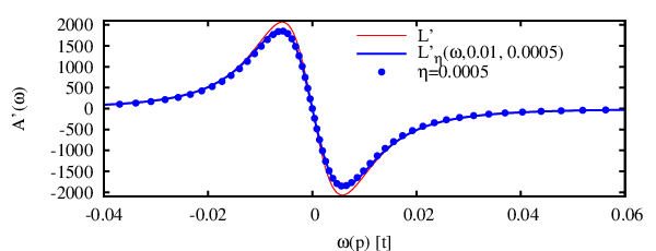
Finally we demonstrate in Figure 11 that within this scheme one can even obtain accurate derivatives of Green functions with respect to the frequency. The derivative of is given by
| (66) | ||||
| (67) |
It turns out that the numerical evaluation of Eqs. (66, 67) is more sensitive to the discretization used. We switch to a linear band, , with cutoffs of , 100 momentum lead sites, the distribution function , , and . As a comparison we plot the exact result and the exact result convoluted with a Lorentzian of half halfwidth ,
| (68) |
By fitting of Eq. (41) to the numerical result we obtain . For the same discretization a fit Eq. (41) of the spectral function gives .
III Bulk Green Functions
In the previous sections we discussed the spectral properties of an impurity, namely a single resonant level, coupled to a non-interacting lead. In this case it was natural to look at the local spectral functions of the impurity. We now turn to the momentum resolved spectral function of a bulk system. As an example we look at the retarded Green function of a tight binding chain
At the spectral function is simply given by .
III.1 Choosing Correct Single Particle States
For simplicity let us start with a sine function ansatz for the single particle states on sites
| (69) | ||||
| (70) |

As can be seen in Figure 12 this ansatz leads to a fictitious double peak structure and an oscillatory part which does not resemble the -peak of the system in the thermodynamic limit. The reason for this is that by using the single particle states of Eqs. (69, 70) we used single particle states which are not eigenstates of the system with periodic boundary conditions (PBC).
Therefore we repeat this calculation for a tight binding chain employing hard wall boundary conditions (HWBC).

The graph in Figure 13 shows that the result looks much better now, but we still obtain the fictitious double peak structure. Again, the reason for this lies in a wrong single particle basis. However, this time the reason for its failure it is more subtle. The problem is that Eq. (70) gives the wrong eigenstates for HWBC and the correct single particle basis is given by
| (71) |
leading to the result of Figure 14 which finally resembles the -peak broadened by .

In summary we would like to point out that one can obtain nice spectral functions for the bulk system from finite system, however care has to be taken to choose the correct representation. Otherwise spurious structures may appear. The need for using the sine solution for HWBC has been pointed out by Benthien, Gebhard, and Jeckelmann[11]. It was shown by Ulbricht and Schmitteckert that for interacting particle in a harmonic trap one can obtain spectral functions from finite system by resorting to hermite polynomials.[12]
IV Poor Man’s Deconvolution: Self Energy Sharpening
In this section we discuss a simple strategy to “sharpen” Green functions obtained in the previous sections. It was first applied to improve the spectral function of a spin polarized ondedimensional Hubbard model.[12] As an example we improve the result for the spectral function of the tight binding chain of the previous section. A straight forward strategy to improve the result consists in a deconvolution to remove the broadening introduced by the finite in the denominator of the resolvents, i.e. perform the inverse operation of Eq. (41). While this procedure is mathematically well defined, it is highly unstable numerically and very sensitive to numerical noise.[13] Here we want to introduce a simple method to improve the results, which has the advantage of being stable and allows to preserve analytical properties of spectral functions, e.g. .
We start by defining the self energy for the infinite system
| (72) |
and the self energy for the finite system which includes the finite broadening
| (73) |
When switching from the infinite system to the finite system we should trace out the discarded part which would lead to a contribution to the self energy of the reduced system. However, we do not know this part. Therefore we make the ansatz that the discarded part can be modeled by the term we already have in the resolvents to enable the mixing of excited states. In this way we obtain our “poor man’s deconvolution” ansatz :
| (74) | ||||
| (75) |
where is the Green function we obtain from our numerics on a finite lattice and is the broadening explicitly used in the numerics. The result of this sharpening applied to the data of Figure 14 is shown in Figure 15. Since real and imaginary part are vanishing up to numerical precision we have rediscovered the -peak structure of the infinite system from the numerics on a finite lattice.

V The NRG Tsunami
Finally we would like to discuss the effect of damped boundary conditions on the dynamics of wave packets to show that boundary conditions are not only important in frequency space, but that they can also change the results in time domain dramatically. In this section we follow the route of [14] adapted for free fermions using exact diagnalization of the quadratic form. In Figure 16 we show the initial states of a 201 site tight binding chain with periodic boundary conditions at half filling, where half a fermion was trapped in the middle of the system by applying a Gaussian potential with a width of . In addition we show the response to the same perturbation for a system where the PBC are replaced by damped boundary conditions, compare Figure 6.

In Figure 17 we show the system after performing a time evolution up to time , in which the homogeneous system moves a distance of sites. Due to the periodic boundary conditions the wave packets appear now at position . Note that by applying a low energy perturbation we create excitations around and our initial wave packet splits into a right and left moving wave packet travelling at , where is the Fermi momentum and is the excitation velocity. However, once the wave packet hits the region of damped boundary conditions (DBC) it sees an exponentially decreasing hopping element which results in an exponentially decreasing excitation velocity. In the similar way as long water waves hitting the shore, where the excitation velocity is decreased, our wave packet has to pile up like a tsunami, since the front is moving much slower than the back. In addition each changed hopping element creates a small back reflection leading to an additional wiggling.

VI Summary
In summary we have shown that one can extract sound results for the thermodynamic limit in the context of calculating Green functions from a finite lattice. However, care has to be taken to choose the correct representation of states. In order to calculate spectral functions at finite frequencies for impurity problems one should apply frequency adapted grids to achieve high resolution. A sharpening procedure based on the self energy can be used as a replacement for deconvoluting the broadening introduced by a finite .
Acknowledgements.
The author wishes to acknowledge assistance and clarifying discussions with Alexander Branschädel, Dan Bohr, Stefan Kremer, Christina Stawiarsky, and Tobias Ulbricht.References
- [1] Gerald D. Mahan. Many particle physics. Kluwer Academics / Plenum Publishers, New York, 3rd edition, 2000.
- [2] Henri Orland and John W. Negele. Quantum Many Particle Systems. Perseus Books, 1998.
- [3] Henrik Bruus and Karsten Flensberg. Many-Body Quantum Theory in Condensed Matter Physics: An Introduction. Oxford University Press, 2004.
- [4] S. Ramasesha. A new algorithm for solving large inhomogeneous linear system of algebraic equations. J. Comp. Chem., page 545, 1990.
- [5] Paolo Longo, Peter Schmitteckert, and Kurt Busch. Few-photon transport in low-dimensional systems: Interaction-induced radiation trapping. Phys. Rev. Lett., page 023602, 2010.
- [6] H. R. Krishna-murthy, J. W. Wilkins, and K. G. Wilson. Renormalization-group approach to the anderson model of dilute magnetic alloys. i. static properties for the symmetric case. Phys. Rev. B, 21(3):1003–1043, Feb 1980.
- [7] M. Vekić and S. R. White. Smooth boundary conditions for quantum lattice systems. Phys. Rev. Lett., 71(26):4283–4286, Dec 1993.
- [8] Dan Bohr and Peter Schmitteckert. Strong enhancement of transport by interaction on contact links. Phys. Rev. B, 75:241103(R), 2007.
- [9] S. Nishimoto and E. Jeckelmann. Density-matrix renormalization group approach to quantum impurity problems. J.Phys.:Condens. Matter, 16:613, 2004.
- [10] Dan Bohr, Peter Schmitteckert, and Peter Wölfle. DMRG evaluation of the Kubo formula – conductance of strongly interacting quantum systems. Europhys. Lett., 73(2):246, 2006.
- [11] H. Benthien, F. Gebhard, and E. Jeckelmann. Spectral function of the one-dimensional Hubbard model away from half filling. Phys. Rev. Lett., 92(25):256401, Jun 2004.
- [12] Tobias Ulbricht and Peter Schmitteckert. Tracking spin and charge with spectroscopy in spin-polarised 1d systems. 2009.
- [13] Carsten Raas and Götz Uhrig. Spectral densities from dynamic density-matrix renormalization. EPJ, 45:293, 2005.
- [14] Peter Schmitteckert. Nonequilibrium electron transport using the density matrix renormalization group. Phys. Rev. B, 70:121302(R), 2004.