The Hunt for New Physics at the Large Hadron Collider
(a) Department of Physics, Northeastern University, Boston, MA 02115, USA
(b) Department of Physics, Brookhaven National Laboratory, Upton, NY 11973, USA
(c) Department of Physics, Texas A&M University, College Station, TX 77843-4242, USA
(d) Michigan Center for Theoretical Physics, Randall Lab., University of Michigan, Ann Arbor, MI 48109
(e) C.N. Yang Institute for Theoretical Physics, Stony Brook University, Stony Brook, NY 11794, USA
(f) Department of Physics, University of Wisconsin, Madison, WI 53706, USA
(g) Institute for Advanced Study ,Princeton, NJ 08540
(h) Maryland Center for Fundamental Physics and Department of Physics, University of Maryland, College Park, MD, 20742
(i) AHEP Group, Instituto de Física Corpuscular – C.S.I.C./Universitat de València, Campus de Paterna, Aptdo 22085, E–46071 València, Spain
(j) School of Physics and Astronomy, University of Manchester, Manchester M13 9PL, United Kingdom
(k) LAL, Université Paris-Sud, IN2P3/CNRS, Orsay, France
(l) Department of Applied Mathematics and Theoretical Physics, Wilberforce Road, Cambridge, CB3 0WA, United Kingdom
(m) Departamento de Física Teórica y del Cosmos and CAFPE, Universidad de Granada, E-18071 Granada, Spain
(n) Department of Physics, University of Wisconsin-Milwaukee, Milwaukee, WI 53201, USA
(o) Dept. of Physics and Astronomy, University of Oklahoma, Norman, OK, 73019, USA
(p) J. Stefan Institute, 1000 Ljubljana, Slovenia
(q) CERN, CH-1211 Genève 23, Switzerland
(r) Theoretical Physics Department, Fermilab, Batavia, IL 60510, USA
(s) EFI and Physics Department, University of Chicago 5640 S. Ellis Ave., Chicago, IL 60637, USA
(t) Fermi National Accelerator Laboratory, P.O. Box 500, Batavia, Illinois 60510, USA
(u) Physics Department, University of Illinois at Chicago, Chicago, Illinois 60607-7059, USA
(v) Physics Department, University of California Davis, Davis, CA 95616
(w) Physics Department, KAIST, Daejeon, 305-701, Korea
(x) Institute for High Energy Phenomenology, Laboratory of Elementary Particle Physics, Cornell University, Ithaca, NY 14853, USA
(y) Departamento de Física e Química, Universidade Estadual Paulista, Guaratinguetá – SP, Brazil
(z) Antwerp University, B-2610 Wilrijk, Belgium
(aa) Physikalisches Institut, Universität Freiburg, Germany
(ab) Instituto de Física, Universidade de São Paulo, São Paulo – SP, Brazil
(ac) University of Vienna, Faculty of Physics, Boltzmanngasse 5, A–1090 Vienna, Austria
(ad) Institut für Physik (THEP), Johannes Gutenberg-Universität, D-55099 Mainz, Germany
(ae) Instituto de Física de Cantabria (CSIC-UC), E–39005 Santander, Spain
(af) Department of Physics, Faculty of Science, University of Alexandria, Alexandria, Egypt
(ag) INFN, Laboratori Nazionali di Frascati, Via E. Fermi 40, I–00044 Frascati, Italy
(ah) SLAC National Accelerator Laboratory 2575 Sand Hill Rd., Menlo Park, CA, 94025, USA
(ai) LAPP, Université de Savoie, IN2P3/CNRS, Annecy, France
(aj) Department of Physics, Brown University, 182 Hope St, Providence, RI 02912, USA
(ak) Technical University of Lisbon, Centre for Theoretical Particle Physics, 1049-001 Lisbon, Portugal
(al) Physics Division, National Center for Theoretical Sciences, Hsinchu, Taiwan
(am) Department of Particle Physics, Weizmann Institute of Science, Rehovot 76100, Israel
(an) Max–Planck–Institut für Physik, Werner–Heisenberg–Institut, 80805 München, Germany
(ao) Arnold Sommerfeld Center for Theoretical Physics, Ludwig-Maximilians-Universität München, 80333 München, Germany
(ap) Centro Universitário Fundação Santo André, Santo André – SP, Brazil
(aq) Theoretical Particle Physics Group, Department of Theoretical Physics, Royal Institute of Technology (KTH), Roslagstullsbacken 21, SE-106 91 Stockholm, Sweden
(ar) Center for Particle Physics and Phenomenology, Université Catholique de Louvain Chemin du Cyclotron 2, B-1348, Louvain-la-Neuve, Belgium
(as) Institut für Theoretische Physik, Universität Karlsruhe, KIT, D–76128 Karlsruhe, Germany
(at) Regional Centre for Accelerator-based Particle Physics, Harish-Chandra Research Institute, Chhatnag Road, Jhunsi, Allahabad - 211 019, India
(au) School of Physics and Astronomy, University of Minnesota, Minneapolis, Minnesota 55455, USA
(av) Institut für Theoretische Physik, Universität Heidelberg, Germany
(aw) Department of Physics, Columbia University, New York, NY 10027, USA
(ax) Institut für Theoretische Physik und Astronomie, Universität Würzburg, D-97074 Würzburg, Germany
(ay) Instituto de Física, Universidad de Antioquia, A.A 1226, Medellin, Colombia
(az) Institute for Particle Physics, ETH Zürich, CH-8093 Zürich, Switzerland
(ba) CAFPE and Departamento de Física Teórica y del Cosmos, Universidad de Granada, E-18071 Granada, Spain
(bb) Department of Physics, Syracuse University, Syracuse, NY 13244-1130, USA
(bc) International Centre for Theoretical Physics, 34100 Trieste, Italy
(bd) Paul Scherrer Institut, CH–5232 Villigen PSI, Switzerland
(be) Department of Biological, Chemical, and Physical Sciences, Illinois Institute of Technology, 3101 S. Dearborn St., Chicago, IL 60616-3793, USA
(bf) Department of Physics and Astronomy, University of California, Irvine, CA 92697, USA
(bg) Dept. of Physics and Astronomy, University of Hawaii, Honolulu, HI , USA
(bh) KICP, University of Chicago 5640 S. Ellis Ave., Chicago, IL 60637, USA
(bi) HEP Division, Argonne National Laboratory 9700 S. Cass Ave., Argonne, IL 60439, USA
(bj) Department of Physics, Princeton University, Princeton, NJ. 08544, USA
(bk) IPPP, University of Durham, Durham DH1 3LE, United Kingdom
The Hunt for New Physics at the Large Hadron Collider
Abstract
The Large Hadron Collider presents an unprecedented opportunity to
probe the realm of new physics in the TeV region and shed light on
some of the core unresolved issues of particle physics. These
include the nature of electroweak symmetry breaking, the origin of
mass, the possible constituent of cold dark matter, new sources of
CP violation needed to explain the baryon excess in the universe,
the possible existence of extra gauge groups and extra matter, and
importantly the path Nature chooses to resolve the hierarchy
problem - is it supersymmetry or extra dimensions. Many models of
new physics beyond the standard model contain a hidden sector which
can be probed at the LHC. Additionally, the LHC will be a top
factory and accurate measurements of the properties of the top and
its rare decays will provide a window to new physics. Further,
the LHC could shed light on the origin of neutralino masses if the
new physics associated with their generation lies in the TeV region.
Finally, the LHC is also a laboratory to test the hypothesis of TeV
scale strings and D brane models. An overview of these possibilities
is presented in the spirit that it will serve as a companion to the
Technical Design Reports (TDRs) by the particle detector groups
ATLAS and CMS to facilitate the test of the new theoretical ideas
at the LHC. Which of these ideas stands the test of the LHC data
will govern the course of particle physics in the subsequent
decades.
Chapter 1 Introduction
Pran Nath
The Large Hadron Collider (LHC) when fully operational will have an
optimal center of mass energy in proton -proton collisions of TeV
and a design luminosity of . The main
experiments at the LHC are: ALICE, ATLAS, CMS, LHCb, and TOTEM. Of
these ALICE is devote to the study of heavy ion collisions, LHCb to
the study of B physics, and TOTEM to the study of total cross
section, elastic scattering and diffraction dissociation at the LHC.
Thus ATLAS11
1
A Torroidal LHC ApparatuS. and
CMS22
2
Compact Muon Solenoid. are the primary detectors
dedicated to the discovery of new physics. It is expected that
initially LHC will run at TeV to collect data for
calibration, later ramping the CM energy to TeV,
and then to TeV.
The particle physics capabilities of the ATLAS and CMS detectors
are described in
their technical design reports (TDRs) [1, 2]
which give an overview of their performance as the LHC begins its operation.
The purpose of the present document is to present a broad overview
of the new physics possibilities that the LHC is likely to see. Of
course, irrespective of the particular nature of new physics the end
product at the LHC would be an excess of observed leptons, photons,
jets and missing energy in some combination. It is then necessary to
devise ways in which one may connect the observed deviations from
the Standard Model prediction to the underlying new physics.
Thus the underlying theme of this report is to provide an overview for experimentalists of the testable new physics at the LHC. The main topics covered in the report are the following.
- 1.
Hunt for supersymmetry
- 2.
Hunt for the Higgs boson
- 3.
CP violation at the LHC
- 4.
LHC and dark matter
- 5.
Top quark physics at the LHC
- 6.
physics at the LHC
- 7.
Visible signatures from the hidden sector at the LHC
- 8.
Probing the origin of neutrino mass at the LHC
- 9.
Hunt for extra dimensions at the LHC
- 10.
Hunt for strings at the LHC
We discuss below each of these topics briefly.
1.1 Hunt for supersymmetry
Supersymmetry provides a technically natural solution to the so
called gauge hierarchy problem that arises in the non-supersymmetric
unified theories with various mass scales. Gauging of
supersymmetry necessarily requires gravity and the gauged
supersymmetry known as supergravity can be coupled to matter and to
Yang Mills gauge fields providing a framework for model building.
The effective potential in supergravity coupled with chiral matter
and gauge fields is not positive definite allowing for the
possibility of fine tuning the vacuum energy to be small. Various
mechanisms exist for the spontaneous breaking of supersymmetry. They
include gravity mediation, gauge mediation and anomaly
mediation and other possible schemes which combine them.
With R parity the lightest supersymmetric particle (LSP) is absolutely stable, and thus production and decays of supersymmetric particles with R parity necessarily involve at least a pair of LSPs. Two of the leading candidates for the LSP are the neutralino and the gravitino both of which are charge neutral and thus also candidates for dark matter. The production and decay of sparticles will thus contain an even number of LSPs and result in significant missing energy. There are many possible signatures available for the discover of supersymmetry at the LHC. The details of the SUSY signatures depend on the specific scenario of SUSY breaking, i.e., gravity mediation, gauge mediation or anomaly mediation or combinations thereof. They are briefly discussed in this report.
1.2 Hunt for the Higgs boson
In the SM there is just one Higgs doublet and thus after spontaneous breaking of the electroweak symmetry, where and become massive, there is only one residual neutral Higgs boson left. However, in the MSSM one has two Higgs doublets, and after spontaneous breaking one is left with four residual Higgs bosons. Of these three are neutral with two CP even Higgs , one CP odd Higgs , and a charged Higgs . Within the MSSM framework, for a broad class of soft breaking with scale O(TeV). The mass of the lightest Higgs boson is limited from above by about 150 GeV. The Higgs boson will certainly be probed at the LHC and the Higgs phenomenology explored in considerable detail.
1.3 CP violation at the LHC
The Standard Model of particle interactions has two sources of CP
violation, one that enters in the Cabibbo-Kobayashi-Maskawa (CKM)
matrix and the other that enters in the strong interaction
dynamics. These phases are constrained by the neutron electric
dipole moment (edm). However, it is known that the CP violation in
the standard model is not sufficient to generate the desired baryon
asymmetry in the universe and new sources of CP violation are
needed. Such new sources can arise in new physics models. Thus,
for example, softly broken supersymmetric theories contain a large
number of new sources of CP violation which can be large and still
consistent with the experimental constraints on the edms of the
electron and of the neutron as well as with the edms of Mercury and of Thallium.
Large CP phases affect the Higgs sector of MSSM leading to a mixing
between the CP even and the CP odd neutral Higgs bosons. Such
mixings can lead to interesting signatures which can be observed at
the LHC. A test of new sources of CP violation can be done in
several other processes such as in sparticle productions and decays
and in signatures including counting signatures and kinematical
signatures as in missing energy, and tranverse momenta of leptons
and jets. Thus the LHC is an excellent laboratory for the discovery
of new sources of CP violation some of which
may enter in the analyses of baryogenesis.
1.4 LHC and dark matter
Current estimates indicate that as much as 96% of the physical universe consists of objects other than the normal (atomic) form of matter while the remainder is constituted of either dark energy () or cold dark matter () [126]. Most main stream approaches to physics beyond the standard model contain possible candidates for cold dark matter. Thus, e.g., in supergravity based models with R parity, the LSP is often a neutralino and thus a candidate for cold dark matter. Similarly, in extra dimension models the lightest Kaluza -Klein particle (LKP) could be a possible dark matter candidate. These massive dark particles would carry a lot of missing energy and can be probed at the LHC. Thus the production of dark particles can be detected and even their masses and their interactions measured with a significant degree of accuracy. For instance, for the neutralino LSP theoretical estimates show that purely from the LHC measurements with about 30 fb-1 of LHC data one can make predictions on the relic density with the same degree of uncertainty as the Wilkinson Microwave Anisotropy Probe (WMAP). Thus from the LHC data alone one would be able to shed light on one of the great mysteries, i.e., the composition of cold dark matter in the Universe.
1.5 Top physics at the LHC
LHC would also be a top factory. Thus the LHC data will provide an accurate determination of the top mass, its couplings and its spin correlations. Additionally the phenomenology of the top can provide a window to new physics via study of its rare decays and via modifications of its couplings from new physics at the loop level, or from a study of top events in associated production.
1.6 physics at the LHC
Another area of considerable interest is the study of additional bosons. Such bosons occur in a variety of extensions of the Standard Model, including grand unified models, strings and branes, extra dimension models and models utilizing alternative schemes of symmetry breaking. If such bosons exist with masses in the TeV region they can be explored at the LHC.
1.7 Visible signatures from the hidden sector at the LHC
In a broad class of particles physics models, including models based on strings and branes, one has a new sector of physics, often labeled the hidden sector (HS), which is typically a gauge singlet under the standard model gauge group. However, communication with the hidden sector may occur in a variety of ways including fields which connect with the visible and the hidden sector, e.g., via kinetic mixing, mass mixing or via higher dimensional operators. In this circumstance signatures exist which can be explored at the LHC. Some hidden sector models also produce a boson which, however, can be very narrow with width which could be just a fraction of a GeV. The possible observation of such a narrow resonance would be a clear indication of a hidden sector and possibly of an underlying string framework.
1.8 Probing the origin of neutrino mass at the LHC
A very interesting possibility not fully appreciated is that the LHC may also be helpful in shedding light on the origin of neutrino mass for which evidence now exists via neutrino oscillations in solar and atmospheric neutrino data along with data from reactors and accelerators. However, the origin of neutrino mass which is much smaller than the masses of the other elementary particles, such as of the electron or of the muon, remains a mystery. If the new physics that generates such a mass lies in the TeV region, it could be explored at the LHC.
1.9 Hunt for extra dimensions at the LHC
Models with a large extra dimension offer an alternative to supersymmetry for the solution to the hierarchy problem. These models produce a rich array of signatures which can be tested at the LHC. They include signatures for black holes in models with weak scale quantum gravity, and of Kaluza Klein excitations in models with compactification radii of size 1/TeV with signatures detectable at the LHC in dilepton signals in Drell-Yan processes as well as in jet production.
1.10 Hunt for strings at the LHC
String theory offers the possibility of unifying all the forces of
nature including gravity. Considerable progress has occurred over
the past two and a half decades in decoding the implications of this
theory at low energies. Although there is no single model yet that
can be labeled unique, there are many possibilities some of which
are discussed in this report. These relate to models based on
heterotic strings, on D branes, as well as on M theory. Recently
several works have presented model independent predictions for TeV
scale strings. The signatures from these various possibilities
are discussed and one finds
these models testable at the LHC.
Each of the main sections in this report was organized by a convener (or conveners) who was (were) responsible for synthesizing several individual contributions to that section and providing a summary and a brief abstract. The document contains many diverse ideas and approaches which are often diametrically opposite: such is the case regarding solution to the hierarchy problem, i.e., supersymmetry vs large extra dimensions. Further, even within a section, different authors present their individual, often competitive approaches. Thus the list of names on the face page simply implies that the authors contributed to one or more sections, but there is no implication that they endorse either the write up of the other sections, or for that matter the write ups of other authors even within the same section.
Bibliography
- [1]
G. Aad et al. [ATLAS Collaboration],
“The ATLAS Experiment at the CERN Large Hadron Collider,”
JINST 3 (2008) S08003.
- [2]
CMS Collaboration, “The CMS Physics Technical Design Report,
Volume1,” CERN/LHCC 2006-001 (2006). CMS TDR 8.1, CMS
Collaboration, “The CMS Physics Technical Design Report, Volume2,”
CERN/LHCC 2006-021 (2006). CMS TDR 8.2.
- [3] D. N. Spergel et al., “Wilkinson Microwave Anisotropy Probe (WMAP) three year results: Implications for cosmology,” astro-ph/0603449. E. Komatsu et al. [WMAP Collaboration], “Five-Year Wilkinson Microwave Anisotropy Probe (WMAP) Observations:Cosmological Interpretation,” Astrophys. J. Suppl. 180, 330 (2009).
Chapter 2 Hunt for Supersymmetry at the LHC
20
Supersymmetry is one of the leading candidates for discovery at the LHC. However, the fact that SUSY partners degenerate with known particles have not been observed requires that supersymmetry must be softly broken in a phenomenologically consistent manner. Many schemes accomplish this prominent among them are the SUGRA grand unified models with gravity mediated breaking, models based on gauge and anomaly mediation and a variety of models using admixtures of the above. In this section we give a brief discussion of some of these topics. We list signatures for weak scale supersymmetry (SUSY) which may be expected at the LHC. From each signature, we provide a description of why the signature might occur, and possible SUSY models which give rise to each specific SUSY signature channel. If new physics is to be discovered at the LHC, the next step would be to reconstruct the underlying theory, and this endeavor should not be biased by any assumption on high-scale models. SFitter and its weighted Markov chain technique is a tool of choice to perform such a task. Using the example of the TeV-scale MSSM Lagrangian we illustrate in detail how it will be possible to analyze this high dimensional physics parameter spaces and extrapolate parameters to the high scale, to test unification. Next in a bottom-up approach, we present global fit results of a phenomenological parametrization of the weak-scale minimal supersymmetric standard model (MSSM) with 25 relevant parameters known as the phenomenological MSSM. Finally, we discuss the recently proposed -kink method to measure the sparticle masses in hadron collider events with missing energy. Here a new kinematic variable, the -Assisted-On-Shell (MAOS) momentum, is introduced which can be useful for spin measurement of new particles produced at the LHC.
2.1 Hunt for SUSY
Pran Nath
Supersymmetry initially postulated in two [1] and then extended to four dimensions [2, 3] possesses the remarkable property of the so called non renormalization theorem [4]. Models based on supersymmetry provide a technically natural solution [5] to the so called gauge hierarchy problem that arises in the non-supersymmetric unified theories with various mass scales. The main problem in building models based on supersymmetry centers around the issue of how to break supersymmetry. One could add to the Lagrangian arbitrary amounts of soft breaking [6]. However, the number of such possibilities is enormous. Thus it is desirable to generate a spontaneous breaking of supersymmetry, which however, turns out to be difficult to achieve in a phenomenologically viable manner within global supersymmetry. Gauging of supersymmetry necessarily brings in gravity [7], leading to a natural fusion of supersymmetry and gravity in supergravity [8]. To build models based on supergravity one needs to couple an arbitrary number of chiral fields and gauge fields in the adjoint representation of the gauge group [9, 10, 11]. Such constructions depend on three arbitrary functions, the superpotential which a holomorphic function of the chiral fields , a Kähler potential for the chiral scalar fields , and the gauge kinetic energy function. One remarkable result of this construction which may be appropriately called applied supergravity is that the scalar potential is not positive definite. This allows one to fine tune the vacuum energy to an arbitrary small value after the breaking of supersymmetry and thus allows one to build phenomenologically viable models based on supersymmetry. Thus the first viable models were build incorporating these features using what is now called gravity mediation [9, 12, 13, 14]. In gravity mediation supersymmetry is broken in the hidden sector and communicated via gravity to the visible sector by gravity- generated soft masses. Supergravity grand unified models [9, 13, 14] also exhibit the further remarkable phenomenon that the soft parameters are independent of the grand unification scale. Supersymmetry breaking in this class of models is governed by the ratio where is a mass scale that enters the hidden sector and and thus GeV corresponds to a soft mass of GeV. Such size scales could arise in supergravity, e.g., via gaugino condensation [15]. However, the actual implementation of such a mechanism is rather intricate since it is non-perturbative. One important modification in gaugino condensation is that the soft masses will be typically of size and thus requires a condensation scale of around GeV.
In minimal supergravity the parameters at the GUT scale consist of and where is the universal scalar mass, is the universal gaugino mass, is the universal trilinear coupling, is the universal bilinear coupling and is the Higgs mixing parameter of the two Higgs doublets, and which give masses to the up quark and to the down quark and the lepton. The parameter arises in supergravity in a natural way and is typically of the size of soft breaking [16]. There exist now several other mechanisms for the breaking of supersymmetry the chief among these are gauge mediation [17, 18] and anomaly mediation [19, 20]. Several other mediation mechanisms have also been discussed in the literature. The phenomenology of the supersymmetric models with soft breaking have been discussed extensively in the literature and some recent reviews can be found in [21, 22],[23],[24, 25, 26].
| mSP | Mass Pattern | |
|---|---|---|
| mSP1 | ||
| mSP2 | ||
| mSP3 | ||
| mSP4 | ||
| mSP5 | ||
| mSP6 | ||
| mSP7 | ||
| mSP8 | ||
| mSP9 | ||
| mSP10 | ||
| mSP11 | ||
| mSP12 | ||
| mSP13 | ||
| mSP14 | ||
| mSP15 | ||
| mSP16 |


One feature which is generic to a variety of schemes is the breaking of the electroweak symmetry by radiative effects [28]. We focus here on the radiative breaking in the context of supergravity models but it can be appropriately adopted for other breaking schemes as well. In SUGRA models one evolves the physical quantities such as gauge couplings, Yukawa couplings and sparticle masses from the GUT scale to low energies by renormalization group [29, 30]. The renormalization group effects then trigger electroweak symmetry breaking reducing to . For the case of the minimal supergravity unified model the magnitude of at the electroweak scale can be determined by using one of the radiative electroweak symmetry breaking conditions, while the parameter can be eliminated in favor of . Thus after the breaking of the electroweak symmetry the parameter space of the minimal supergravity model, mSUGRA , consists of 4 parameters and the sign of , i.e., the parameters [31]
| (2.1) |
One important consequence of the supergravity unification is that it leads to a unification of gauge couplings[32] consistent with the LEP data [152]. Further, the sparticle spectrum can be computed by the renormalization group evolution [34, 35, 36, 37, 38] in terms of the parameters of Eq.(2.1).
| mSP | Mass Pattern | |
|---|---|---|
| mSP17 | ||
| mSP18 | ||
| mSP19 | ||
| mSP20 | ||
| mSP21 | ||
| mSP22 |
| NUSP | Mass Pattern | Model |
|---|---|---|
| NUSP1 | NU3,NUG | |
| NUSP2 | NU3 | |
| NUSP3 | NUG | |
| NUSP4 | NUG | |
| NUSP5 | NU3 | |
| NUSP6 | NU3 | |
| NUSP7 | NUG | |
| NUSP8 | NUG | |
| NUSP9 | NUG | |
| NUSP10 | NUG | |
| NUSP11 | NUG | |
| NUSP12 | NUG | |
| NUSP13 | NUG | |
| NUSP14 | NUG | |
| NUSP15 | NUG |
We note that the nature of physics at the Planck scale is not fully known and thus deformations from universality should be considered. This is what is done in non-universal supergravity models, where one considers modifications of universality consistent with flavor changing neutral currents. The above possibility allows the following sets of allowed non-universalities: (i) non-universalities in the Higgs sector (NUH), non-universalities in the third generation sector (N3q), and (iii) nonuniversalities in the gaugino sector (NUG).
2.1.1 Hyperbolic Branch / Focus Point (HB/FP)
The radiative breaking of the electroweak symmetry exhibits two important branches. One of the these is the conventional branch where the soft parameters lie on the surface of an ellipsoid. For a given amount of fine tuning the soft parameters can move around on the ellipsoid surface but cannot get very large for fixed radii. However, there is another branch the Hyperbolic Branch (HB) where for certain regions of the parameter space the ellipsoid turns into a hyperboloid (see the first paper of [39]). On the hyperbolic branch the scalar masses can get very large (5-10 TeV or even larger) consistent with a small fine tuning and other experimental constraints. This region is also often called the Focus Point region (see the second paper of [39]).
After the breaking of the electroweak symmetry one generates the masses of all the 32 sparticles in terms of a small number of soft parameters, and because of this small number many sum rules on sparticle masses result [40]. The allowed parameter space is limited by a variety of constraints such as color and charge conservation as well as experimental lower limits on sparticle masses from LEP and from the Tevatron. Further, there are constraints arising from the Brookhaven experiment on [41], and from the flavor changing processes , and . Regarding , it in known that the supersymmetric contribution to the anomalous magnetic moment of the muon can be as large or larger than the standard model electroweak contribution [42]. The most recent analysis of gives for the value [43]
| (2.2) |
which is a deviation from the Standard Model. This result is similar to the Brookhaven 2001 result which was about deviation and led to the prediction that there should be upper limits on the sparticle masses[44]. Thus if the result of Eq.(2.2) holds up, it would imply that sparticles must be observed at the LHC.
Regarding the FCNC decay it arises only at loop level and the supersymmetric contributions are typically comparable to the Standard Model contributions. Consequently the difference between the experimental value and the Standard Model value acts as a strong constraint on new physics (For theoretical analyses of this decay in supersymmetry see [45]). The most recent evaluations of the Standard Model result including the next to next leading order contributions to this process give at [46] the result
| (2.3) |
The above is to be compared with the experimental central value given by The Heavy Flavor Averaging Group (HFAG) [47] along with the BABAR, Belle and CLEO experimental results: . The difference between the experiment and the Standard Model result acts as a strong constraint on new physics. The current discrepancy between theory and experiment requires about a correction from supersymmetry which points to the possibility of relatively light charged Higgs, charginos, and stops [48].
Additionally, if one assumes that R parity is conserved, which is what is assumed in a large class of models discussed in the literature, then this results in the lightest sparticle (LSP) being absolutely stable. If the LSP is neutral it is a possible candidate for dark matter. In SUGRA models over most of the allowed parameter space the neutralino turns out to be the LSP [34] and thus a candidate for dark matter [49][50]. More recently other possibilities have also been considered as discussed in the section below.
As mentioned above there are 32 sparticles in the MSSM which after breaking of supersymmetry and after electroweak supersymmetry breaking acquire masses. These masses arrange themselves in a hierarchical pattern and as many as possibilities may arise (depending on additional constraints imposed) leading to a vast landscape of sparticle mass hierarchies. It is interesting to ask how this landscape shrinks within a specific model of soft breaking. The result for the general case of 32 sparticle tower is currently unknown although partial results were given for the mSUGRA case in Ref. [51] However, if one limits oneself to the first four lightest sparticles aside from the LSP and the lightest Higgs boson, then there are only 22 such possibilities in mSUGRA for both signs of which are labeled as the minimal supergravity patterns mSP1-mSP22 [51]. These are exhibited in Table 2.2. Here mSP1-mSP4 are the ones where the next to the lightest particle (NLSP) is the chargino and they can be labeled Chargino Patterns (CP), mSP5-mSP10, mSP17-mSP19 are the ones where NLSP is the stau and they can be labeled Stau Patterns (SUP), mSP11-mSP13, mSP20-mSP21 are the ones where NLSP is the stop and hence they can be labeled Stop Patterns (SOP), mSP14-mSP16 are the ones where NLSP is either the CP odd Higgs or the heavy CP even Higgs and they can be labeled Higgs Patterns (SUP), and finally we have mSP22 where the second neutralino is the LSP and it can be labeled a Neutralino Pattern (NEP). The sign for which these patterns can be realized is listed in the last column of Table 2.2. As may be seen from this table most of the patterns appear for both signs of while a small number appears only for one sign of .
As mentioned already the nature of Planck scale physics is not fully understood and thus it is useful to consider inclusion of non-universalities in the analysis [52, 53, 54, 55, 56, 57, 58]. A similar analysis but including non-universalities is given in Table 2.3 where the last column indicates the type of non-universality [51] Here the patterns corresponding to the lightest four particles are labeled as non-universal SUGRA models NUSP and they range from NUSP1-NUSP15. One interesting new feature is that the gluino can be an NLSP.
Signatures of supersymmetry at colliders have been discussed in many works. Some early work on signatures and search for supersymmetry can be found in [31, 59, 60] and an early review on the search for supersymmetric particles in hadron-hadron collisions is [61] and a more recent review is given in [62]. Many interesting questions arise regarding such searches, e.g., how one distinguishes SUSY from extra dimensions [63, 64], how one can extrapolate back from the LHC data to hopefully a unique point in the parameter space of a new physics model [71, 73, 74], how well one can measure sparticle masses [41, 58, 70] and what one may learn from the early runs at the LHC [71, 72, 73, 74, 75].
An illustration of how an appropriate combination of signatures can discriminate among models is given in Fig.(2.1). The left panel of Fig.(2.1) exhibits the allowed parameter space of the mSUGRA model (used here as an illustration) in the plane under the constraints of radiative breaking, naturalness assumptions, and under WMAP and other experimental constraints. Using this parameter space the right panel of Fig.(2.1) exhibits the discrimination of the Chargino, Higgs, Stau, and Stop Patterns in the signature space of the fraction vs the fraction with 10 fb-1 of LHC data at TeV. The analysis shows the sparticle patterns can be easily discriminated from the Standard Model background and further they can also be discriminated from each other in most cases. Of course a full discrimination among models would require a combination of many signatures. A more complete list of such signatures can be found in [71, 51] and a more detailed discussion of sparticle signatures is given below.
2.2 A Brief Catalogue of SUSY Signatures at the LHC
Howard Baer and Xerxes Tata
We list signatures for weak scale supersymmetry (SUSY) which may be
expected at the LHC. From each signature, we provide a description
of why the signature might occur, and possible SUSY models
which give rise to each specific SUSY signature channel.
Particle physics models that include weak scale supersymmetry (supersymmetric matter at the weak scale: GeV) are highly motivated by both theory and experiment [25, 26]. A generic prediction of such models is the existence of new matter states – the superpartners of ordinary matter – with the same gauge quantum numbers as ordinary matter, but spins differing by 1/2, and masses in the GeV range. The CERN Large Hadron Collider (LHC) is a proton-proton collider which is expected to begin operating in November, 2009, with the start-up energy of TeV increasing to 8-10 TeV in 2010, with the ultimate goal of running at its design energy of 14 TeV. With such high energies, production cross sections for TeV-scale new matter states with SM gauge interactions, such as the SUSY superpartners or heavy Higgs bosons, should be at an observable level.
In SUSY models with a conserved -parity, heavy sparticles produced at LHC decay to lighter sparticles plus Standard Model (SM) particles until this cascade terminates in the lightest SUSY particle (LSP) which is stable. This is also the case in -parity violating models if these -violating couplings are small compared with gauge couplings, except that then the would-be-stable LSP also decays into SM particles. By including sparticle production reactions, sparticle decay channels, initial and final state QCD radiation, hadronization, and beam remnant modeling, one can predict using event generator programs the sorts of collider events expected from SUSY, along with various SM background processes.
How superpartners acquire SUSY-breaking masses and couplings is unknown, and a generic parametrization requires 178 parameters [25], making phenomenology intractable. Various economic models, with mass patterns and corresponding characteristic collider signatures have been constructed. Here, we catalogue a wide variety of LHC SUSY signatures together with associated SM background sources, and list the SUSY models from which they might arise.
SUSY models divide into three main classes characterized by the SUSY breaking mediation mechanism:
- •
Models with gravity-mediated SUSY breaking (SUGRA), where supergravity is broken by a GeV in a “hidden sector” resulting in a massive gravitino. The gravitino mass sets the overall mass scale for the superpartners, and is expected to be at or around the TeV-scale [10, 12, 13, 76]. Three well-motivated LSP candidates include: 1. the lightest neutralino (a WIMP dark matter candidate) 2. the gravitino itself [77] (although constraints from gravitino overproduction and Big Bang Nucleosynthesis must be respected) and 3. if the Peccei-Quinn solution to the strong problem is invoked, the axino [78, 79] (here, dark matter might then consist of an axion/axino admixture [80]). Active sneutrinos are disfavored, while gauge singlet sneutrinos are another possibility [81].
- •
Gauge-mediated SUSY breaking models [17, 18] (GMSB) contain a hidden sector which interacts with a messenger sector, and where the messenger sector experiences SM gauge forces. If messengers are relatively light, the SUSY breaking scale can be low, and the gravitino mass () can be of order eV-GeV, in which case it is the LSP.
- •
Anomaly-mediated SUSY breaking models [19, 20] (AMSB) include a hidden sector geometrically separated from the visible sector in extra dimensions, suppressing the tree level contribution to SM superpartner masses and the loop level SUSY breaking Weyl anomaly contribution dominates. The gravitino is expected to be 1-2 orders of magnitude heavier than the TeV scale. AMSB needs to be augmented by an additional source of SUSY breaking to avoid a tachyonic slepton. A wino-like neutralino is usually the LSP.
Combinations of SUSY-breaking mediation mechanisms [82] that can lead to very interesting phenomenology [83] are also possible.
2.2.1 Catalogue of SUSY signatures
Unless gluinos and squarks are very heavy, one expects copious gluino and/or squark production at the LHC [84]. Gluinos can decay either via two-body modes or three body modes or . Squarks almost always decay via the two body modes: or, for left-squarks, also via . In special cases, loop-level decays of sparticles may also be important [85, 86]. Gluino/squark production generically leads to multi-jet plus multilepton (from decays of daughter and ) with, in -parity conserving models, also large from the undetected LSPs and sometimes also from neutrinos. Recently, correlations between sparticle mass patterns and ensuing signatures have been examined [56, 51].
2.2.2 Events with missing
Jets with charged lepton veto
This is the classic SUSY signature in all -parity conserving models. The dominant background comes from QCD multi-jet production, where arises from missed jets, or hadronic energy mis-measurement. This background is detector-dependent. Important physics backgrounds come from production where , production where (), and the lepton is mis-measured, soft or non-isolated [87] and production where again the leptons from the decay are mismeasured or soft or not isolated. Numerous other SM hard scattering backgrounds exist, usually at lower rates. The hard and spectrum coming from the heavy SUY particles usually allows for signal to be distinguished from BG in that signal has a much harder distribution in , , or .
jets
In most models, cascade decays of gluinos and squarks to s or s, with or (), occur without a big rate suppression because the lepton can come from any one of many decay chains. Requiring a hard isolated lepton gets rid of much of QCD BG, but leaves BG from processes such as and production [88].
Opposite sign (OS) dilepton jets
Gluino and squark cascade decays readily lead to a pair of hard isolated different flavor where mostly each lepton originates in a chargino, or the same flavor or where the leptons come from either a single neutralino or a pair of charginos in the decay cascade, along with jets and . The neutralino contribution is statistically isolated in the flavor-subtracted cross section. Then, the dilepton invariant mass is kinematically bounded by for decays from (though for small values of contributions from are also identifiable). If neutralinos decay to real sleptons the mass edge occurs instead at
The dilepton mass edge [89] is a smoking gun for SUSY cascade decays and often serves as a starting point for the reconstruction of decay chains [90], assuming the neutralino leptonic branching fraction is large. SM backgounds to the OS dilepton signal from neutralinos mainly come from (followed by ), and pair production.
Same sign (SS) dilepton jets
Majorana gluinos are equally likely to decay into positive/negative charginos via so that gluino pair production followed by the cascade decay of both gluinos leads to SS, isolated dilepton plus jets plus events [91, 92]. This signature also arises from and production followed by cascade decays. In fact, since LHC is a collider, then a charge asymmetry in vs. events is expected if or production is dominant, while no charge asymmetry is expected from production [92, 88]. SM BGs come from production (where one lepton from a decay is lost, production, or processes such as production and are much smaller than in the OS dilepton channel.
jets
Gluino and squark cascade decays also lead to three-isolated lepton plus jet events, albeit with a lower rate. These events are nonetheless important because as isolated lepton multiplicity increases, SM backgrounds usually drop much more rapidly than SUSY signal. This makes it possible to use the trilepton signal to pick out SUSY signals from SM backgrounds in early stages of LHC running when reliable measurements are not possible [72, 73, 74]. SM BGs include production, where one of the semi-leptonic decays yields a hard, isolated lepton, together with other processes.
jets
Multi-jet events with isolated leptons are ubiquitous in GMSB models where the selectron/smuon/stau are together the next-to-lightest SUSY particle (NLSP) produced as the penultimate step in the SUSY decay cascade. The NLSP then decays via into the gravitino LSP so that every SUSY event has at least two leptons (and frequently more). The SM background to lepton events (where the leptons do not reconstruct the mass is very small, and in this case LHC experiments can probe gluino masses up to 3 TeV with just 10 fb-1 of integrated luminosity [93] to be compared with a reach of TeV in the corresponding case where the LSP escapes the detector undetected.
- and -jets in SUSY events
Gluino and squark cascade decays are often expected to be rich in -jets, so these can be used to reduce SM backgrounds. There are several reasons [94]: 1) large top and botom Yukawa couplings– especially at large – enhance decays to third generation quarks, especially if has significant higgsino content as favored by the measured density of cold dark matter, 2) in many models third generation squarks are lighter than other squarks, resulting in an enhancement of sparticle decays to -quarks, and 3) real or virtual Higgs bosons, produced in cascade decays, dominantly decay to - and -quarks. -jet tagging thus allows an increased SUSY reach at the LHC, in models with first generation squarks substantially heavier than gluinos [93].
An enhanced multiplicity of leptons, identified by their decays to 1 or 3 charged particles, is expected in SUSY cascade decay events at large , for much the same reasons as high multiplicities are expected [96].
Leptonic bosons in SUSY events
In the case where either , or have significant branching fractions (frequently so for the former if is suppressed), then cascade decay events containing real events are expected at high rates [97] compared to SM BGs from , or production, especially if high jets and are also required in the signal.
Higgs bosons in SUSY events
It is entirely possible that the the lightest Higgs scalar will be discovered first in the SUSY cascade rather than via usual SM search strategies that limit the search to its rare decays. The reason is that with hard jet and cuts it is possible to search for via a mass bump in its dominant [98] (and also the ) decay mode without being overwhelmed by QCD backgrounds.
Heavy Higgs bosons and can sometimes also be produced in SUSY cascade decay events [99]. It may be possible to reconstruct mass bumps such as . Also, heavy Higgs decay to SUSY particles is sometimes possible, such as if . This would impact upon searches for heavy Higgs bosons via their decays to SM particles.
2.2.3 Jet-free multilepton events
OS-dilepton
Clean trilepton
Electroweak production of charginos and neutralinos via , followed by and decay [102] yields clean trilepton events for which SM backgrounds are very small. The signal is largest and readily observable over background when and are wino-like and the spoiler decay modes are kinematically closed. The OS dilepton mass edge from the decay should again be visible, corroborating its SUSY origin.
2.2.4 Signals with isolated photons
In GMSB models with a gravitino LSP and the next-to-lightest SUSY particle (NLSP), is often the dominant decay mode of . Then, gluino and squark production followed by their cascade decays will always yield at least two s, both of which decay to hard, isolated photons. Thus, GMSB models with a small number of messenger fields are expected to yield large rates for multi-jet multi-lepton events [103].
Hard isolated photons can also arise in SUGRA-type models, where the branching fraction for the loop decay is significant [86]. These loop decays are enhanced if the - mass gap is small as in small models or in models with at the weak scale [104], where the 3-body decays of are strongly suppressed by phase space.
In some cases, if production is large in cascade decay events, then the decay can be reconstructed in the SUSY event sample [105].
2.2.5 Signals from long-lived charged sparticles
Highly ionizing tracks (HITs)
In the simplest GMSB models with large enough number of messenger fields, the slepton (usually the lighter stau ) is the NLSP. The NLSP then decays via will take place, but with a rate suppressed by its tiny coupling to the goldstino component of . In such a case, the relatively slow-moving heavy is long-lived, and leaves a highly ionizing track as it traverses the detector. These tracks may terminate, or leave a kink, depending on where the delayed NLSP decay occurs. A determination of the NLSP lifetime, and hence the fundamental SUSY breaking scale, is possible if the NLSP decay length is between 0.5 m to 1 km [106]. The wino-like chargino of AMSB models has a decay length of order centimeters and so leaves a short stubby track potentially with kinks from its pion daughter.
Trapping sleptons
If the gravitino is heavy enough, the charged slepton NLSP of GMSB models may live days or months or even longer. In this case, it is possible to capture these sleptons produced in collider experiments in, for instance, a water tank surrounding the detector. The water can be siphoned off, and the slepton decay properties can then be well-measured: e.g. its lifetime, and mass (based on energy release from an at-rest slepton decay) [107].
An intriguing variant of this idea is to trigger on events with GeV and high jet activity that contain an isolated track from a slow-moving stau (or any charged massive particle, the CHAMP) stopped in the calorimeter, and at this stage dump the beams (or at least change their orbit) so there are no collisions (in at least the triggered detector) for about an hour, during which the focus is on the detection of the decay products of CHAMPs trapped in the calorimeter [108] if the lifetime is 1 hour. Longer-lived CHAMPs can be studied during collider shut-downs. It is claimed that, with an integrated luminosity of 100 fb-1, stau lifetimes ranging from s will be measureable at ATLAS, and that this idea may be extendable to other quasi-stable CHAMPs.
2.2.6 Events with displaced vertices
In the case of GMSB models with a long-lived neutralino LSP decaying via , or or , the decay vertex will be dispaced from the primary interaction point and the EM shower induced by the or the decay products of the or will likely not point back to the interaction point. The same is true for a neutralino LSP decaying via tiny -parity violating couplings. The case of the photon decay of has been studied in detail [109] and it was shown that for an NLSP decay length of 10 cm-20 m, the secondary vertex could be well-determined from events where the photon converts to an electron-positron pair so that reconstruction of the entire SUSY event is possible. It is claimed that this reconstruction is also possible using events where the photon does not convert, since the degradation in the precision is compensated by the much larger number of events. The NLSP lifetime is determined to within a few percent. This is an important measurement as it determines the fundamental scale of SUSY breaking.
2.2.7 Events containing intermittent tracks
Scenarios with stable [110] or long-lived [111] gluinos or squarks (usually ) have been considered. Once produced at colliders, the squark or gluino quickly hadronizes by picking up an antiquark or a gluon/, respectively, and traverses the detector as an -hadron that may be electrically charged or neutral. This -hadron interacts with nuclei in the detector material via pion exchanges, and so may move between its charged and neutral states, thereby manifesting itself as an intermittent track in a collider event: a track that suddenly appears, disappears and reappears along its path [112, 110]. In the quasi-stable particle case, the intermittent track might terminate in a burst of hadronic showers which of course would not point back to the interaction region.
2.2.8 Inclusive multilepton events without
In -parity violating models where the LSP decays into SM particles, neutrinos are the only physics source of and the classic signature is greatly reduced (though even in the worst-case scenario where the LSP decays hadronically, the 10 fb-1 reach extends to 1 TeV in [113]. In the favorable case that the neutralino LSP decays purely leptonically via , SUSY events will be awash in multileptons and the reach will be greatly increased even without . There are no reach calculations available for the LHC, but even the Tevatron is sensitive to mSUGRA parameter values that give GeV [114]. Event shapes in the OS dilepton channel (especially dilepton mass distributions) [115] and the rate for SS dilepton production [116] at the LHC are sensitive to -parity violating interactions,.
2.2.9 Resonance sparticle production
In -parity violating scenarios with -type couplings, it is possible to resonantly produce sleptons and sneutrinos at the LHC [117]. The phenomenology is very sensitive to details of the model, and potentially to interesting multilepton signals. Even assuming just a single -parity violating coupling, the phenomenology depends on the scale at which this single coupling is assumed to be present, since renormalization effects induce small (but phenomenologically significant) values for other -violating couplings at the weak scale. For a recent analysis, see Ref. [118], and references therein.
2.2.10 Rapity gap events from SUSY
Very recently [119] it has been pointed out that production of squark pairs by -channel exchanges of colour singlet -inos would lead to events with large “rapidity gaps”, i.e. little energy deposition between squark decay products. If this observation survives scrutiny and such events turn out to be observable, they could be used to separate electroweak squark pair production from the much larger QCD squark pair production, and provide a new, potentially interesting ways to separate SUSY contributions at the LHC.
2.2.11 Final Remarks
We have listed a number of signals via which SUSY may be discovered at the LHC. While some of the catalogued signals are quite generic, and so present in wide classes of models, others occur only in specific scenarios, or only for special regions of model parameter space. Seeing a signal in several channels will corroborate that the origin of the new physics is supersymmetry, while their relative rates (together with measurements of masses, branching ratios, etc.) will serve to zero in on the underlying framework. Observation of special signatures will be particularly useful as these occur only in specific models.
2.3 LHC Measurements
Claire Adam-Bourdarios, Remi Lafaye, Tilman Plehn, Michael Rauch, and Dirk Zerwas
If new physics is to be discovered at the LHC, the next step would
be to reconstruct the underlying theory, and this endeavor should
not be biased by any assumption on high-scale models. SFitter
[120] and its weighted Markov chain technique is a tool of
choice to perform such a task.11
1
Fittino [121]
follows a very similar logic to SFitter, including a scan of the
high dimensional MSSM parameter space. Using the example of the
TeV-scale MSSM Lagrangian we illustrate in detail how it will be
possible to analyze this high dimensional
physics parameter spaces and extrapolate parameters to the high scale, to test unification.
The analysis critically depends on detailed experimental simulations of measurements and errors at the LHC. Therefore the well-understood parameter point SPS1a [122] is used.
The parameter point SPS1a is characterized by moderately heavy squarks and gluinos, which leads to long cascades including neutralinos and sleptons. Gauginos are lighter than Higgsinos, and the mass of the lightest Higgs boson is close to the mass limit determined at LEP. At the LHC, the mass measurements are obtained from measurements of kinematical endpoints and mass differences. The particle mass measurements used by SFitter [120] are taken from Ref. [123], while the central values are calculated by SuSpect [124].
In order to obtain reliable error estimates for the fundamental parameters, a proper treatment of experimental and theory errors depending on their origin is mandatory. The CKMfitter prescription [125] is largely followed. The complete set of errors includes statistical experimental errors, systematic experimental errors, and theory errors.
The statistical experimental errors are treated as uncorrelated among the measured observables, in contrast to the systematic experimental errors, essentially due to the uncertainty in the lepton and jet energy scales, expected to be 0.1% and 1%, respectively, at the LHC. These energy-scale errors are each taken to be 99% correlated. Theory errors are propagated from the masses to the measurements and are not taken to be gaussian but flat box-shaped. Thus, the probability assigned to any measurement does not depend on its actual value, as long as it is within the interval covered by the theory error. Outside this interval, normal statistical and systematic errors treatment is used.
2.3.1 mSUGRA
mSUGRA is an example of a model with few parameters, most of which are defined at the grand unification scale (GUT).
SFitter approaches the problem of the high dimensional parameter space, producing first a set of Markov chains over the entire parameter space. Then, Minuit resolves the local maxima in the likelihood map. Once the global best fitting parameter point is identified, the errors on all parameters are determined using smeared sets of pseudo measurements and flat theory errors [120].
The precision obtained with LHC alone is at the level of percent for the determination of the parameters. It is improved by the ILC by about an order of magnitude. Including the theoretical errors has an impact on the precision at both machines, the errors are larger by a factor of three to four. Thus the precision of the parameter determination at the LHC is limited by the precision of the theoretical predictions.


2.3.2 MSSM
The complete parameter space of the MSSM can have more than 100 parameters. However, at experiments like the LHC some new physics parameters can be fixed, because no information on them is expected. Properly including phenomenological constraints and leads to an effective 19-dimensional parameter space.
LHC provides 22 measurements, counting the measurements involving separately for electrons and muons. Using these naively it should be possible to completely constrain a 19-dimensional parameter space. However, the situation is more complicated. These 22 measurements are constructed from only 15 underlying masses. The additional measurements will resolve ambiguities and improve errors, but they will not constrain any additional parameters.
SFitter approaches the problem of the higher dimensional MSSM parameter space by an iterative procedure. With LHC measurements only, eight solutions are found. The errors obtained for one of the minima, the one closest to the SPS1a point, are shown in Table 2.4 : while many parameters are well determined, some model parameters turn out to be not well constrained. Some of them, namely the trilinear mixing terms , are fixed in the fit because their impact is close to zero. Others, like the heavier stau-mass and stop-mass parameters or the pseudoscalar Higgs mass, turn out to be unconstrained because they do not appear directly in any of the measurements.
| fixed 0 | |||
| fixed 0 | |||
| fixed 0 | fixed 0 | ||
| fixed 0 | |||
All values are given in GeV.
Moreover, there is no good direct measurement of . Looking at the neutralino and sfermion mixing matrices, any effect in changing can always be accommodated by a corresponding change in another parameter. Here, information from flavour physics or the anomalous magnetic moment of the muon can help [126].
2.3.3 Extrapolation to High Scale
The MSSM is defined at the electroweak scale. The definition of its parameters does not depend on the model of supersymmetry breaking. Thus, having determined the parameters at the weak scale, the extrapolation of the parameters to the GUT scale can be performed, using RGE’s : instead of assuming unification at the GUT scale as in mSUGRA, it can now be tested.
Figure 2.2 shows that, for the point chosen in Table 2.4, unification is observed. However, this is only true for one of the 8 solutions : with LHC only, requiring unification can be used to reduce the number of degenerate solutions, but cannot be proven.
In conclusion a sophisticated tool such as SFitter is necessary to
determine the underlying parameters of supersymmetry from the
correlated measurments of the LHC. mSUGRA can be determined at
the percent level, and most of the MSSM parameters are measured
precisely. The MSSM parameters can be extrapolated to the GUT scale
to test grand unification for possibly degenerate solutions.
2.4 Fits to the Phenomenological MSSM
Sehu S AbdusSalam, Benjamin Allanach, Fernando Quevedo
With the LHC experiments about to start we are at a new and exciting scientific era where enquiries about the fundamentals of nature will be governed by experiments and hence complement the past decades of theoretically motivated efforts. A great deal of research directed towards understanding the origin of SUSY breaking from ultra-violet theories lead to a plethora of models but no single one clearly favoured over the others. Many of them, however, fall into some subset of the phenomenologically viable MSSM parameter space.
For a phenomenological MSSM (pMSSM) fit, the source of SUSY breaking is completely decoupled from the problem such that all relevant parameters are varied simultaneously at the weak energy scale. This is a general approach to SUSY breaking phenomenology and has been studied in [87]. Here we present a summary of the pMSSM global fit construction and results.
Only real soft SUSY breaking terms were considered, with all off-diagonal elements in the sfermions mass terms and trilinear couplings set to zero, and the first and second generation soft terms equalised. The effects of the trilinear coupling terms , , on SUSY effects are not negligible. So also , which is relevant for the computation of the anomalous magnetic moment of the muon, . pMSSM Higgs-sector parameters are specified by , , and . Important SM parameters we varied are , , , and .
The above parameters form a vector, , such that the combined prior PDF for the model (H = pMSSM) is . Two widely different, the linear and log, priors were used to check the robustness of the fits.
The constraints employed include the -boson mass, , the effective leptonic weak mixing angle, , the total -boson decay width, , , Z-pole asymmetry parameters and the mass of the lightest MSSM Higgs boson, ; branching ratios , , , and the mass-mixing parameter ; and the dark matter relic density from WMAP5 results. These make the dataset .
The set of pMSSM predictions, , for the above observables were obtained from the 25 input parameters, sampled using MultiNest [78], in the SLHA format [82] via SOFTSUSY2.0.17 [81] for producing the MSSM spectrum; micrOMEGAs2.1 [83] for computing neutralino dark matter relic density, the branching ratio and ; SuperIso2.0 [84] for predicting the Isospin asymmetry in the decays and with all NLO SUSY QCD and NNLO SM QCD contributions included; and susyPOPE [85] for computing -boson mass , the effective leptonic mixing angle variable , the total -boson decay width, and other Z-pole asymmetry parameters from processes.
The combined likelihood from the different predictions of the observables , together with the prior PDF via the Bayes’ theorem, Eq. 2.4, is used to compute the posterior PDF of the parameters, observables and predictions for the MSSM SUSY mass spectrum.
| (2.4) |
where and are respectively the experimental central values and errors.
We found that the sparticle mass spectrum for the log prior assumption can have slepton, squarks and neutralino LSP masses as low as about 251 GeV, 383 GeV and 243 GeV respectively. The masses are much heavier for the linear prior assumption as expected. The Higgs boson mass turned out to be approximately prior independent with an almost equal mass range of about GeV to GeV for both prior assumptions.
| (a) | (b) | (c) | (d) |
|---|---|---|---|

|

|

|

|
The statistical pulls of the various observables are shown in Fig. 2.3 at the best-fit point. We see from the figure that, like the Standard Model, the forward-backward asymmetry in provides the greatest discrepancy, being at odds with data at the level. Notably, an extra-SM component of the and the relic density of cold dark matter, are well fit. Both quantities are ill-fitting in the Standard Model.
We now summarise the marginalised posterior PDFs for various pMSSM quantities, but the full set of plots can be found in Ref. [87]. Some differences between the posterior PDFs for the two prior cases can be observed. They are mostly due to the fact that the sparticle masses are larger in the linear prior measure, leading to a suppression of SUSY effects in the loop calculations of most observables. As such, only the EW physics observables show significant difference between the two prior cases while the other observables (except for, notably, the DM constraint) are relatively weaker in constraining the parameter space. Linear pMSSM global fit results show a mild preference for , depending on the constraint. However, there is no conclusive evidence for one particular over the other.
The gluino-neutralino mass ratio quantifies the amount of visible energy that could be seen in sparticle production from LHC collisions and therefore could be used to discriminate between different models. mSUGRA (AMSB) with predominantly bino (wino) LSP predicts 6(and 9) [88]. The mirage mediation [89] and the LARGE volume [71, 72] scenarios have the characteristic ratio less than 6 and between 3 to 4 respectively. However by construction, the pMSSM is a more generic approach for MSSM phenomenology. We show the pMSSM posterior PDFs for the gluino-neutralino mass ratio in Fig. 2.4(a). The linear prior predicts a compact while for the log prior a much broader distribution mostly around 10.
The amount of fine-tuning in the pMSSM is quantified by considering the sensitivity of to parameter variations , where and are the relevant parameters. The over-all measure of fine-tuning, , is
| (2.5) |
Values of far greater than unity indicate large fine-tuning. As shown in Fig. 2.4(b) fine-tuning typically mild for either prior measure. The log prior has a lower because SUSY breaking terms are much reduced compared to the linear prior case.

 |
The LSP neutralino mass eigenstate is a mixture of bino (), wino() and Higgsino () gauge fields with real coefficients
| (2.6) |
Gaugino/Higgsino admixture PDFs of the LSP are shown in Fig. 2.4(c). The LSP is almost purely Higgsino with a neutralino-chargino dominant co-annihilation channel in the linear prior case. For log priors, it is an admixture of mostly gaugino and to a much lesser extent Higgsino with a neutralino-slepton dominant co-annihilation channel. Thus, current data do not unambiguously constrain the LSP.
An independent sampling with the WMAP relic density constraint used only as an upper bound (i.e. allowing for non LSP DM components) favours very low DM relic densities, typically in the range , compared to the case of purely LSP DM assumption, as shown in Fig. 2.4(d). Thus once one allows an additional component of DM to the LSP, the model prefers the additional component to dominate the relic density.
The pMSSM global fit results are also consistent with DM direct detection bounds although current data are insufficient to constrain the direct detection cross-sections. The constraint from the cryogenic cold dark matter search (CDMS) experiments on the pMSSM is shown in Fig. 2.5.
The strong prior dependence of the fits is a measure of the insufficient information from experimental data to derive robust results about the preferred SUSY parameter space. In any case this type of study would be most relevant and needed in the near future once more information about possible SUSY extension of the SM is obtained at LHC experiments.
2.5 Mass and Spin Measurement with the Transverse Mass Variable
Kiwoon Choi
2.5.1 Introduction
-parity conserving supersymmetry (SUSY) predicts a clear signature at the LHC: excessive multi-jet (possibly with isolated leptons) events with a large missing transverse momentum, which are due to pair-produced squarks or gluinos subsequently decaying to the invisible lightest supersymmetric particle (LSP) through model-dependent decay chains. It is highly challenging to determine the masses and spins of sparticles in such events because of missing kinematic information. In recent years, several methods to measure the unknown masses or spins in hadron collider events with missing energy have been proposed [139]. Here we briefly discuss the methods that rely on the kinematic variable [140, 141, 142, 143, 144].
2.5.2 Kink
A typical SUSY event at the LHC takes the form:
| (2.7) | |||||
where denote pair-produced (mother) sparticles each of which decays to a set of visible SM particles () and the invisible LSP (), and stands for visible particles not coming from . The event variable [140] is defined as
| (2.8) |
where the transverse mass is given by for generic trial LSP mass and trial transverse momentum , , , and the missing transverse momentum is given by . For each event, the corresponding is a monotonically increasing function of , and its value at is bounded as
| (2.9) |
where and are the true masses of and , respectively. Then, generically there can be multiple events that saturate the above upper bound at , but have different values of . This simple observation implies that the endpoint values of generically exhibit a kink [141, 142] at .
In Fig. 2.6, we depict for some events with , and , when . The curve (a) stands for an event with , , (b) is for , and (c) is for , . They show that the kink can be sharp enough if is a multi-particle state having a wide range of and/or is large enough to be of . There are some cases known to give a visible kink [141, 142], e.g. (i) in heavy sfermion scenario, for which , and (ii) for which a large is provided by the gluino/squark decay producing . It remains to be seen if the -kink method can be applied to a wider class of SUSY events.

2.5.3 MAOS Momentum
The -Assisted-On-Shell (MAOS) momentum is an event variable designed to systematically approximate the invisible LSP momentum in the SUSY event (2.7) [143]. The transverse components, and , correspond to the trial LSP transverse momenta which determine , while the longitudinal and energy components are determined by the on-shell conditions:
| (2.10) |
An interesting feature of the MAOS momentum is that it corresponds to the true LSP momentum for the endpoint events of . This indicates that the MAOS momentum might provide a reasonable approximation to the true LSP momentum even for generic non-endpoint events, and the approximation can be systematically improved by selecting an event subset near the endpoint. This can be confirmed by Fig. (2.7) showing the distribution of
| (2.11) |
for the gluino pair decays: in the focus point scenario of mSUGRA. Here the dotted line is the distribution over the full event set, while the solid line is the distribution over the 10% subset near the endpoint.

In certain cases, the MAOS momenta can be useful for spin measurement [143]. For instance, for the 3-body decay , the gluino spin can be easily read off from , where and or . One can also determine the slepton spin with the production angle distribution obtained from for . MAOS momentum can be used also to determine the Higgs boson mass in [144].
Bibliography
- [1] P. Ramond, Phys. Rev. D 3, 2415 (1971).
- [2] Yu A. Golfand and E.P. Likhtman, JETP Lett. 13, 452 (1971); D. Volkov and V.P. Akulov, JETP Lett. 16, 438 (1972).
- [3] J. Wess and B. Zumino, Phys. Lett. B 49, 52 (1974); Nucl. Phys. B 70, 39 (1974);
- [4] J. Iliopoulos and B. Zumino, Nucl. Phys. B 76, 310 (1974); M. Grisaru, M. Roĉek and W. Seigel, Nucl. Phys. B159, 429 (1979).
- [5] S. Dimopoulos and H. Georgi, Nucl. Phys. B 193, 150 (1981); N. Sakai, Z. Phys. C 11, 153 (1981).
- [6] L. Giradello and M. T. Grisaru, Nucl. Phys. B194 65 (1982).
- [7] P. Nath and R. Arnowitt, Phys. Lett. B 56, 177 (1975); R. Arnowitt, P. Nath and B. Zumino, Phys. Lett. B 56, 81 (1975).
- [8] D. Z. Freedman, P. van Nieuwenhuizen and S. Ferrara, Phys. Rev. D 13, 3214 (1976); S. Deser and B. Zumino, Phys. Lett. B 62, 335 (1976).
- [9] A. H. Chamseddine, R. L. Arnowitt and P. Nath, Phys. Rev. Lett. 49 (1982) 970.
- [10] E. Cremmer, S. Ferrara, L. Girardello and A. Van Proeyen, Nucl. Phys. B 212 (1983) 413.
- [11] P. Nath, R. L. Arnowitt and A. H. Chamseddine, “Applied N=1 Supergravity,” world scientific,1984.
- [12] R. Barbieri, S. Ferrara and C. A. Savoy, Phys. Lett. B 119 (1982) 343.
- [13] L. J. Hall, J. D. Lykken and S. Weinberg, Phys. Rev. D 27 (1983) 2359.
- [14] P. Nath, R. L. Arnowitt and A. H. Chamseddine, Nucl. Phys. B 227 (1983) 121.
- [15] H. P. Nilles, Phys. Lett. B115, 193 (1981); S. Ferrara, L. Girardello and H. P. Nilles, Phys. Lett. B125, 457 (1983).
- [16] G. F. Giudice and A. Masiero, Phys. Lett. B 206 (1988) 480.
- [17] M. Dine, A. E. Nelson, Y. Nir and Y. Shirman, Phys. Rev. D 53 (1996) 2658.
- [18] G. F. Giudice and R. Rattazzi, Phys. Rept. 322 (1999) 419.
- [19] L. Randall and R. Sundrum, Nucl. Phys. B 557 (1999) 79.
- [20] G. F. Giudice, M. A. Luty, H. Murayama and R. Rattazzi, JHEP 9812 (1998) 027 [arXiv:hep-ph/9810442].
- [21] H. P. Nilles, Phys. Rept. 110, 1 (1984).
- [22] H. E. Haber and G. L. Kane, Phys. Rept. 117 (1985) 75.
- [23] S. P. Martin, arXiv:hep-ph/9709356.
- [24] P. Nath, arXiv:hep-ph/0307123.
- [25] H. Baer and X. Tata, “Weak scale supersymmetry: From superfields to scattering events,” Cambridge, UK: Univ. Pr. (2006) 537 p
- [26] M. Drees, R. Godbole and P. Roy, Hackensack, USA: World Scientific (2004) 555 p; P. Binetruy, Supersymmetry, (Oxford, 2007).
- [27] D. Feldman, Z. Liu and P. Nath, Phys. Rev. Lett. 99, 251802 (2007); [arXiv:0707.1873 [hep-ph]].
- [28] K. Inoue et al., Prog. Theor. Phys. 68, 927 (1982); L. Ibañez and G. G. Ross, Phys. Lett. B110, 227 (1982); L. Alvarez-Gaumé, J. Polchinski and M. B. Wise, Nucl. Phys. B250, 495 (1983).
- [29] M. E. Machacek and M. T. Vaughn, Nucl. Phys. B 222, 83 (1983); Nucl. Phys. B 236, 221 (1984); Nucl. Phys. B 249, 70 (1985).
- [30] S. P. Martin and M. T. Vaughn, Phys. Lett. B 318, 331 (1993); Phys. Rev. D 50, 2282 (1994); I. Jack, D. R. Jones, S. P. Martin, M. T. Vaughn and Y. Yamada, Phys. Rev. D 50, 5481 (1994).
- [31]
For some early work on SUGRA models see
S. Weinberg, Phys. Rev. Lett. 50, 387 (1983); R. Arnowitt, A. H. Chamseddine and P. Nath, Phys. Rev. Lett. 50 (1983) 232; A. H. Chamseddine, P. Nath and R. Arnowitt, Phys. Lett. B 129, 445 (1983); P. Nath, R. Arnowitt and A. H. Chamseddine, HUTP-83/A077; D. A. Dicus, S. Nandi, W. W. Repko and X. Tata, Phys. Rev. Lett. 51, 1030 (1983); Phys. Rev. D 29, 67 (1984); Phys. Rev. D 29, 1317 (1984); D. A. Dicus, S. Nandi and X. Tata, Phys. Lett. B 129, 451 (1983); J. M. Frere and G. L. Kane, Nucl. Phys. B 223, 331 (1983); J. R. Ellis, J. M. Frere, J. S. Hagelin, G. L. Kane and S. T. Petcov, Phys. Lett. B 132, 436 (1983). - [32] S. Dimopoulos, S. Raby and F. Wilczek, Phys. Rev. D 24, 1681 (1981).
- [33] J. Ellis, S. Kelley and D. V. Nanopoulos, Phys. Lett. 249B, 441 (1990); B260, 131 (1991); U. Amaldi, W. de Boer and H. Furstenau, Phys. Lett. 260B, 447 (1991); P. Langacker and M. x. Luo, Phys. Rev. D 44, 817 (1991); F. Anselmo, L. Cifarelli, A. Peterman and A. Zichichi, Nuov. Cim. 104A, 1817 (1991).
- [34] R. L. Arnowitt and P. Nath, Phys. Rev. Lett. 69 (1992) 725.
- [35] G. G. Ross and R. G. Roberts, Nucl. Phys. B 377 (1992) 571.
- [36] V. D. Barger, M. S. Berger and P. Ohmann, Phys. Rev. D 49 (1994) 4908.
- [37] G. L. Kane, C. F. Kolda, L. Roszkowski and J. D. Wells, Phys. Rev. D 49 (1994) 6173.
- [38] H. Baer, M. Drees, C. Kao, M. Nojiri and X. Tata, Phys. Rev. D 50 (1994) 2148 [arXiv:hep-ph/9403307].
- [39] K. L. Chan, U. Chattopadhyay and P. Nath, Phys. Rev. D 58 (1998) 096004; J. L. Feng, K. T. Matchev and T. Moroi, Phys. Rev. Lett. 84, 2322 (2000); H. Baer, C. Balazs, A. Belyaev, T. Krupovnickas and X. Tata, JHEP 0306, 054 (2003); For a review see, A. B. Lahanas, N. E. Mavromatos and D. V. Nanopoulos, Int. J. Mod. Phys. D 12, 1529 (2003).
- [40] S. P. Martin and P. Ramond, Phys. Rev. D 48, 5365 (1993).
- [41] G. W. Bennett [Muon g-2 Collaboration], arXiv:hep-ex/0208001.
- [42] T. C. Yuan, R. Arnowitt, A.H. Chamseddine and P. Nath, Z. Phys. C26, 407(1984); D. A. Kosower, L. M. Krauss, N. Sakai, Phys. Lett. 133B, 305(1983); J. Lopez, D.V. Nanopoulos, and X. Wang, Phys. Rev. D49, 366(1994); U. Chattopadhyay and P. Nath, Phys. Rev. D53, 1648(1996); T. Moroi, Phys. Rev. D 53, 6565 (1996).
- [43] M. Davier, A. Hoecker, B. Malaescu, C. Z. Yuan and Z. Zhang, arXiv:0908.4300 [hep-ph].
- [44] J. L. Feng and K. T. Matchev, Phys. Rev. Lett. 86, 3480 (2001); E. A. Baltz and P. Gondolo, Phys. Rev. Lett. 86, 5004 (2001); L. L. Everett, G. L. Kane, S. Rigolin and L. T. Wang, Phys. Rev. Lett. 86, 3484 (2001); U. Chattopadhyay and P. Nath, Phys. Rev. Lett. 86, 5854 (2001); T. Ibrahim, U. Chattopadhyay and P. Nath, Phys. Rev. D64, 016010(2001); J. Ellis, D.V. Nanopoulos, K. A. Olive, Phys. Lett. B 508, 65 (2001); R. Arnowitt, B. Dutta, B. Hu, Y. Santoso, Phys. Lett. B 505, 177 (2001); S. P. Martin, J. D. Wells, Phys. Rev. D 64, 035003 (2001); H. Baer, C. Balazs, J. Ferrandis, X. Tata, Phys.Rev.D64: 035004, (2001).
- [45] S. Bertolini, F. Borzumati and A. Masiero, Phys. Rev. Lett. 59, 180(1987); G. Degrassi, P. Gambino and G. F. Giudice, JHEP 0012 (2000) 009; F. Borzumati, C. Greub, T. Hurth and D. Wyler, Phys. Rev. D 62, 075005 (2000); M. E. Gomez, T. Ibrahim, P. Nath and S. Skadhauge, Phys. Rev. D 74 (2006) 015015; G. Degrassi, P. Gambino and P. Slavich, Phys. Lett. B 635 (2006) 335.
- [46] M. Misiak et al., Phys. Rev. Lett. 98 (2007) 022002.
- [47] E. Barberio et al. [Heavy Flavor Averaging Group], arXiv:0808.1297 [hep-ex].
- [48] N. Chen, D. Feldman, Z. Liu and P. Nath, arXiv:0911.0217 [hep-ph].
- [49] H. Goldberg, Phys. Rev. Lett. 50, 1419 (1983); J. Ellis, J.S. Hagelin, D.V. Nanopoulos, and M. Srednicki, Phys. Rev. Lett. 127B, 233(1983).
- [50] M.W. Goodman and E. Witten, Phys. Rev. D31, 3059(1983); A. K. Drukier, K. Freese and D. N. Spergel, Phys. Rev. D 33, 3495 (1986); K. Freese, J. A. Frieman and A. Gould, Phys. Rev. D 37, 3388 (1988); K.Greist, Phys. Rev. D38, (1988)2357.
- [51] D. Feldman, Z. Liu and P. Nath, JHEP 0804, 054 (2008).
- [52] J.R. Ellis, K. Enqvist, D.V. Nanopoulos and K. Tamvakis, Phys. Lett. B 155, 381 (1985); M. Drees, Phys. Lett. B 158, 409 (1985); G. Anderson, C.H. Chen, J.F. Gunion, J.D. Lykken, T. Moroi and Y. Yamada, [hep-ph/9609457].
- [53] P. Nath and R. L. Arnowitt, Phys. Rev. D 56, 2820 (1997); R. L. Arnowitt, B. Dutta and Y. Santoso, Nucl. Phys. B 606, 59 (2001); J. R. Ellis, T. Falk, K. A. Olive and Y. Santoso, Nucl. Phys. B 652, 259 (2003); D. G. Cerdeno and C. Munoz, JHEP 0410, 015 (2004).
- [54] A. Corsetti and P. Nath, Phys. Rev. D 64, 125010 (2001); U. Chattopadhyay and P. Nath, Phys. Rev. D 65, 075009 (2002); A. Birkedal-Hansen and B. D. Nelson, Phys. Rev. D 64, 015008 (2001); A. Birkedal-Hansen and B. D. Nelson, Phys. Rev. D 67, 095006 (2003); U. Chattopadhyay and D. P. Roy, Phys. Rev. D 68, 033010 (2003); G. Belanger, F. Boudjema, A. Cottrant, A. Pukhov and A. Semenov, Nucl. Phys. B 706, 411 (2005); I. Gogoladze, R. Khalid, N. Okada and Q. Shafi, arXiv:0811.1187 [hep-ph]; S. Bhattacharya, A. Datta and B. Mukhopadhyaya, Phys. Rev. D 78, 115018 (2008); M. E. Gomez, S. Lola, P. Naranjo and J. Rodriguez-Quintero, JHEP 0904, 043 (2009); U. Chattopadhyay, D. Das and D. P. Roy, Phys. Rev. D 79, 095013 (2009); S. Bhattacharya and J. Chakrabortty, arXiv:0903.4196 [hep-ph].
- [55] H. Baer, A. Mustafayev, S. Profumo, A. Belyaev and X. Tata, JHEP 0507, 065 (2005).
- [56] G. Anderson, H. Baer, C. h. Chen and X. Tata, Phys. Rev. D 61, 095005 (2000) [arXiv:hep-ph/9903370].
- [57] K. Choi and H. P. Nilles JHEP 0704 (2007) 006;
- [58] B. Altunkaynak, P. Grajek, M. Holmes, G. Kane and B. D. Nelson, arXiv:0901.1145 [hep-ph];
- [59] H. Baer, K. Hagiwara and X. Tata, Phys. Rev. D 35 (1987) 1598.
- [60] P. Nath and R. L. Arnowitt, Mod. Phys. Lett. A 2 (1987) 331.
- [61] S. Dawson, E. Eichten and C. Quigg, Phys. Rev. D 31 (1985) 1581.
- [62] J. L. Feng, J. F. Grivaz and J. Nachtman, arXiv:0903.0046 [hep-ex].
- [63] A. Datta, G. L. Kane and M. Toharia, arXiv:hep-ph/0510204.
- [64] J. M. Smillie and B. R. Webber, JHEP 0510 (2005) 069 [arXiv:hep-ph/0507170].
- [65] N. Arkani-Hamed, G. L. Kane, J. Thaler and L. T. Wang, JHEP 0608 (2006) 070.
- [66] B. Altunkaynak, M. Holmes and B. D. Nelson, JHEP 0810 (2008) 013.
- [67] C. Balazs and D. Kahawala, arXiv:0904.0128 [hep-ph].
- [68] R. L. Arnowitt, B. Dutta, A. Gurrola, T. Kamon, A. Krislock and D. Toback, Phys. Rev. Lett. 100, 231802 (2008).
- [69] R. L. Arnowitt et al., Phys. Lett. B 649, 73 (2007); R. L. Arnowitt, B. Dutta, T. Kamon, N. Kolev and D. A. Toback, Phys. Lett. B 639, 46 (2006).
- [70] M. M. Nojiri, Y. Shimizu, S. Okada and K. Kawagoe, JHEP 0806 (2008) 035.
- [71] J. Hubisz, J. Lykken, M. Pierini and M. Spiropulu, Phys. Rev. D 78 (2008) 075008.
- [72] H. Baer, H. Prosper and H. Summy, Phys. Rev. D 77 (2008) 055017.
- [73] H. Baer, A. Lessa and H. Summy, Phys. Lett. B 674 (2009) 49.
- [74] H. Baer, V. Barger, A. Lessa and X. Tata, J. High Energy Phys. 0909 (2009) 063.
- [75] J. Edsjo, E. Lundstrom, S. Rydbeck and J. Sjolin, arXiv:0910.1106 [hep-ph].
- [76] N. Ohta, Prog. Theor. Phys. 70, 542 (1983).
- [77] H. Pagels and J. Primack, Phys. Rev. Lett. 48 (1982) 223; J. Feng, A. Rajaraman and F. Takayama, Phys. Rev. Lett. 91 (2003) 011302 and Phys. Rev. D 68 (2003) 085018.
- [78] K. Rajagopal, M. Turner and F. Wilczek, Nucl. Phys. B 358 (1991) 447; H. Baer, A. D. Box, arXiv:0910.0333 [hep-ph]
- [79] L. Covi, J. E. Kim and L. Roszkowski, Phys. Rev. Lett. 82 (1999) 4180; L. Covi, H. B. Kim, J. E. Kim and L. Roszkowski, J. High Energy Phys. 0105 (2001) 033. L. Covi, L. Roszkowski and Small, J. High Energy Phys. 0207 (2002) 023.
- [80] H. Baer, A. Box and H. Summy, J. High Energy Phys. 0908 (2009) 080.
- [81] See e.g. T. Asaka, K. Ishiwata and T. Moroi, Phys. Rev. D 75 (2007) 065001.
- [82] A. Pomarol and R. Rattazzi, J. High Energy Phys. 9905 (1999) 013; K. Choi et al. J. High Energy Phys. 0509 (2005) 039; M. Endo et al. Phys. Rev. D 72 (2005) 015004; A. Falkowski et al. J. High Energy Phys. 0511 (2005) 034; L. Everett, I.W. Kim, P. Ouyang and K. Zurek, Phys. Rev. Lett. 101 (2008) 101803.
- [83] R. Rattazzi et al. Nucl. Phys. B 576 (2000) 3; H. Baer et al. J. High Energy Phys. 0706 (033) 2007 and references therein.
- [84] P. R. Harrison and C. H. Llewellyn Smith, Nucl. Phys. B 213 (1983) 223; [61]; H. Baer and X. Tata, Phys. Lett. B 160 (1985) 159.
- [85] E. Ma and G. Wong, Mod. Phys. Lett. A 3 (1988) 1561; R. Barbieri et al. Nucl. Phys. B 301 (1988) 15, H. Baer, X. Tata and J. Woodside, Phys. Rev. D 42 (1990) 1568.
- [86] H. E. Haber and D. Wyler, Nucl. Phys. B 323 (1989) 267; H. Komatsu and J. Kubo, Phys. Lett. B 157 (1985) 90; S. Ambrosanio and B. Mele, Phys. Rev. D 53 (1996) 2541 and Phys. Rev. D 55 (1997) 1399 [Erratum-ibid. D56, 3157 (1997)]; H. Baer and T. Krupovnickas, J. High Energy Phys. 0209 (2002) 038.
- [87] H. Baer, C. H. Chen, F. Paige and X. Tata, Phys. Rev. D 52 (1995) 2746; S. Abdullin and F. Charles, Nucl. Phys. B 547 (1990) 60; CMS Collaboration, arXiv: hep-ph/9806366; S. Bityukov and N. Krasnikov, Phys. Lett. B 469 (1999) 469; ATLAS Collaboration, Detector and Physics Performance: Technical Design Report ; CMS Collaboration, Physics Technical Design Report, V. 2 (2006).
- [88] H. Baer, C. H. Chen, F. Paige and X. Tata, Phys. Rev. D 53 (1996) 6241.
- [89] [59]; H. Baer, D. Dzialo-Karatas and X. Tata, Phys. Rev. D 42 (1990) 2259; H. Baer, C. Kao and X. Tata, Phys. Rev. D 48 (1993) 5175; H. Baer, C. H. Chen, F. Paige and X. Tata, Phys. Rev. D 50 (1994) 4508.
- [90] I. Hinchliffe, F. Paige, M. Shapiro, J. Soderqvist and W. Yao, Phys. Rev. D 55 (1997) 5520 and Phys. Rev. D 60 (1999) 095002; H. Bachacou, I. Hincliffe and F. Paige, Phys. Rev. D 62 (2000) 015009.
- [91] R. M. Barnett, J. Gunion and H. E. Haber, Phys. Rev. Lett. 315 (1993) 349.
- [92] H. Baer, X. Tata and J. Woodside, Phys. Rev. D 45 (1992) 142.
- [93] H. Baer, P. Mercadante, X. Tata and Y. Wang, Phys. Rev. D 62 (2000) 095007.
- [94] H. Baer, C. Chen, M. Drees, F. Paige and X. Tata, Phys. Rev. Lett. 79 (1997) 986 and Phys. Rev. D 59 (1999) 015010.
- [95] U. Chattopadhyay et al. Phys. Lett. B 493 (2000) 127; P. Mercadante et al. Phys. Rev. D 72 (2005) 035009; S.P. Das et al. Eur. Phys. J. C 54 (2008) 645; R. Kadala et al. Eur. Phys. J. C 56 (2008) 511.
- [96] For tau detection, see A. Kalinowski, Nucl. Phys. B 189 (2005) 305 (Proc. Suppl); for taus in SUSY events, see C. Zendler, talk at SUSY 2009, ATL-COM-PHYS-2009-265.
- [97] H. Baer, X. Tata and J. Woodside, Phys. Rev. D 42 (1990) 1450;
- [98] H. Baer, M. Bisset, X. Tata and J. Woodside, Phys. Rev. D 46 (1992) 303.
- [99] H. Baer, M. Bisset, D. Dicus, C. Kao and X. Tata, Phys. Rev. D 47 (1993) 1062; H. Baer, M. Bisset, C. Kao and X. Tata, Phys. Rev. D 50 (1994) 316; F. Moorgat, S. Abdullin and D. Denegri, hp-ph/0112046; M. Bisset et al. J. High Energy Phys. 0908 (2009) 037, and references therein.
- [100] H. Baer, C. H. Chen, F. Paige and X. Tata, Phys. Rev. D 49 (1994) 3283.
- [101] A. Barr, J. High Energy Phys. 0602 (2006) 042.
- [102] H. Baer, C. H. Chen, F. Paige and X. Tata, Phys. Rev. D 50 (1994) 4508.
- [103] S. Dimopoulos, S. Thomas and J. D. Wells, Nucl. Phys. B 488 (1997) 39; H. Baer, P. Mercadante, F. Paige, X. Tata and Y. Wang, Phys. Lett. B 435 (1998) 109; H. Baer et al., Ref.[93]
- [104] H. Baer et al. J. High Energy Phys. 0512 (2005) 011.
- [105] H. Baer, C. Balazs, A. Belyaev, T. Krupovnickas and X. Tata, J. High Energy Phys. 0306 (2003) 054.
- [106] ATLAS Technical Design Report, Ref.[87]; S. Ambrosanio et al. J. High Energy Phys. 0101 (2001) 014; see also, K. Hamaguchi et al. Phys. Lett. B 663 (2008) 86 for lifetime determination with very small decay tracks.
- [107] J. L. Feng and B. Smith, Phys. Rev. D 71 (2005) 015004 and Phys. Rev. D 71 (2005) 019904 (E); K. Hamaguchi et al. Phys. Rev. D 70 (2004) 115007 and J. High Energy Phys. 0703 (2007) 046.
- [108] S. Asai, K. Hamaguchi and S. Shirai, Phys. Rev. Lett. 103, 141803 (2009).
- [109] K. Kawagoe et al. Phys. Rev. D 69 (2004) 035003.
- [110] H. Baer, K. Cheung and J. Gunion, Phys. Rev. D 59 (1999) 075002.
- [111] N. Arkani-Hamed and S. Dimopoulos, J. High Energy Phys. 0506 (2005) 073; N. Arkani-Hamed and S. Dimopoulos, G. Giudice and A. Romanino, Nucl. Phys. B 709 (2005) 3; W. Kilian, T. Plehn, P. Richardson and E. Schmidt, Eur. Phys. J. C 39 (2005) 229.
- [112] M. Drees and X. Tata, Phys. Lett. B 252 (1990) 695.
- [113] H. Baer C. Chen and X. Tata, Phys. Rev. D 55 (1997) 1466.
- [114] H. Baer, C. Kao and X. Tata, Phys. Rev. D 51 (1995) 2180.
- [115] D. Choudhury, R. Godbole and G. Polesello, J. High Energy Phys. 0208 (2002) 004.
- [116] A. Bartl et al. Nucl. Phys. B 502 (1997) 19.
- [117] S. Dimopulos and L. Hall, Phys. Lett. B 207 (1988) 210.
- [118] H. Dreiner, S. Grab and M. Trenkel, Phys. Rev. D 79 (2009) 016002; M. Bernhardt et al. Phys. Rev. D 79 (2009) 035003.
- [119] S. Bornhauser et al. arXiv: 0909.2595, and arXiv:0909.5155.
- [120] R. Lafaye, T. Plehn, M. Rauch, D. Zerwas, Eur. Phys. J. C 54, 617 (2008).
- [121] P. Bechtle, K. Desch, W. Porod and P. Wienemann, Eur. Phys. J. C 46, 533 (2006).
- [122] B. C. Allanach et al., Eur. Phys. J. C 25, 113 (2002).
- [123] G. Weiglein et al. [LHC/LC Study Group], Phys. Rept. 426, 47 (2006).
- [124] A. Djouadi, J. L. Kneur and G. Moultaka, arXiv:hep-ph/0211331.
- [125] A. Höcker, H. Lacker, S. Laplace and F. Le Diberder, Eur. Phys. J. C 21, 225 (2001).
- [126] M.M. Nojiri et al. [Les houches 2007 Susy], arXiv:0802.3672 [hep-ph].
- [127] S. S. AbdusSalam, B. C. Allanach, F. Quevedo, F. Feroz, and M. Hobson, arXiv:0904.2548.
- [128] F. Feroz and M. P. Hobson, arXiv:0704.3704; F. Feroz, M. P. Hobson, and M. Bridges, arXiv:0809.3437.
- [129] P. Skands et. al., JHEP 07 (2004) 036, hep-ph/0311123.
- [130] B. C. Allanach, Comput. Phys. Commun. 143 (2002) 305–331, hep-ph/0104145.
- [131] G. Belanger, F. Boudjema, A. Pukhov, and A. Semenov, Comput. Phys. Commun. 174 (2006) 577–604, hep-ph/0405253.
- [132] F. Mahmoudi, arXiv:0808.3144.
- [133] S. Heinemeyer, W. Hollik, A. M. Weber, and G. Weiglein, JHEP 04 (2008) 039, arXiv:0710.2972.
- [134] S. S. AbdusSalam, arXiv:0809.0284.
- [135] H. P. Nilles in talk at SUSY 2008, Seoul, Korea, 2008.
- [136] O. Lebedev, H. P. Nilles, and M. Ratz, hep-ph/0511320.
- [137] J. P. Conlon, S. S. Abdussalam, F. Quevedo, and K. Suruliz, JHEP 0701 (2007) 032 [arXiv:hep-th/0610129]; J. P. Conlon and F. Quevedo, JHEP 0606 (2006) 029 [arXiv:hep-th/0605141].
- [138] J. P. Conlon, C. H. Kom, K. Suruliz, B. C. Allanach, and F. Quevedo, JHEP 0708 (2007) 061 [arXiv:0704.3403].
- [139] For a recent review, see A. De Roeck et. al. arXiv:0909.3240 [hep-ph].
- [140] C. G. Lester and D. J. Summers, Phys. Lett. B463 (1999) 99 [ hep-ph/9906349]; A. J. Barr, C. G. Lester and P. Stephens, J. Phys. G29 (2003) 2343 [hep-ph/0304226].
- [141] W. S. Cho, K. Choi, Y. G. Kim and C. B. Park, Phys. Rev. Lett. 100 (2008) 171801 [arXiv:0709.0288]; W. S. Cho, K. Choi, Y. G. Kim and C. B. Park, JHEP 0802 (2008) 035 [arXiv:0711.4526].
- [142] B. Gripaios, JHEP 0802, 053 (2008) [arXiv:0709.2740]; A. J. Barr, B. Gripaios and C. G. Lester, JHEP 0802 (2008) 014 [arXiv:0711.4008].
- [143] W. S. Cho, K. Choi, Y. G. Kim and C. B. Park, Phys. Rev. D79 (2009) 031701 [arXiv:0810.4853].
- [144] K. Choi, S. Choi, J. S. Lee, and C. B. Park, arXiv:0908.0079 [hep-ph].
Chapter 3 Higgs Physics
20
3.1 Predictions for SUSY Higgses at the LHC
O. Buchmueller, R. Cavanaugh, A. De Roeck, J.R. Ellis, H. Flächer, S. Heinemeyer, G. Isidori, K.A. Olive, F.J. Ronga and G. Weiglein
One of the main goals of the LHC is the identification of the mechanism of electroweak symmetry breaking. The most frequently investigated models are the Higgs mechanism within the Standard Model (SM) and within the Minimal Supersymmetric Standard Model (MSSM) [1]. Contrary to the case of the SM, in the MSSM two Higgs doublets are required. This results in five physical Higgs bosons instead of the single Higgs boson in the SM. These are the light and heavy -even Higgs bosons, and , the -odd Higgs boson, , and the charged Higgs bosons, . The Higgs sector of the MSSM can be specified at lowest order in terms of the gauge couplings, the ratio of the two Higgs vacuum expectation values, , and the mass of the -odd Higgs boson, . Consequently, the masses of the -even neutral and the charged Higgs bosons are dependent quantities that can be predicted in terms of the Higgs-sector parameters. Higgs phenomenology in the MSSM is strongly affected by higher-order corrections, in particular from the sector of the third generation quarks and squarks, so that the dependencies on various other MSSM parameters can be important, see e.g. [2, 3, 4] for reviews. The mass of the lightest Higgs boson is bounded from above by [5]. For the other Higgs bosons are close to each other, .
Predictions for the MSSM Higgs bosons masses, which are needed to evaluate the LHC discovery potential, are bedeviled by the large dimensionality of the MSSM. For this reason, simplifying assumptions that may be more or less well motivated are often made, so as to reduce the parameter space to a manageable dimensionality. We focus here on the framework of the constrained MSSM (CMSSM), in which the soft supersymmetry-breaking scalar and gaugino masses are each assumed to be equal at some GUT input scale. In this case, the new independent MSSM parameters are just four in number: the universal gaugino mass , the scalar mass , the trilinear soft supersymmetry-breaking parameter , and the ratio of Higgs vacuum expectation values. The pseudoscalar Higgs mass and the magnitude of the Higgs mixing parameter can be determined by using the electroweak vacuum conditions, leaving the sign of as a residual ambiguity. An extension of the CMSSM is obtained in the NUHM1 in which the soft SUSY-breaking contributions to the Higgs masses are allowed a different but common value with respect to the scalar fermion mass parameter . Effectively this yields either or as an additional free parameter at the electroweak (EW) scale.
3.1.1 Frequentist Fit
We will review the results for the predictions of Higgs boson masses and other properties of the Higgs sector in the CMSSM and NUHM1, based on a frequentist approach [6]. In our frequentist analysis we use the Markov chain Monte Carlo (MCMC) technique to sample efficiently the CMSSM and NUHM1 parameter spaces, and we generate sufficiently many chains to sample these parameter spaces completely.
Our treatments of the experimental constraints from electroweak precision observables, -physics observables and cosmological data are explained in detail in [6, 7, 8]. We define a global likelihood function, which combines all theoretical predictions with experimental constraints:
| (3.1) | |||||
Here is the number of observables studied, represents an experimentally measured value (constraint) and each defines a prediction for the corresponding constraint that depends on the supersymmetric parameters. The constraints comprise a variety of electroweak precision observables (e.g., , and (LEP), , , …), flavour related observables (e.g., BR(), BR(), …) and the relic abundance of cold dark matter (CDM), , see [6] for details. The experimental uncertainty, , of each measurement is taken to be both statistically and systematically independent of the corresponding theoretical uncertainty, , in its prediction. The three standard model parameters are included as fit parameters and allowed to vary with their current experimental resolutions . We do not include , which would have only a minor impact on the analysis.


3.1.2 Results for


We start the discussion of predictions by showing the likelihood functions for within the CMSSM and NUHM1 frameworks obtained when dropping the contribution to from the direct Higgs searches at LEP, shown in the left and right panels of Fig. 3.1, respectively. It is well known that the central value of the Higgs mass in a SM fit to the precision electroweak data lies below 100 GeV [9], but the theoretical and experimental uncertainties in the SM fit are such that there is no significant discrepancy with the direct lower limit of 114.4 GeV [10, 38] derived from searches at LEP. In the case of the CMSSM and NUHM1, one may predict on the basis of the underlying model parameters, with a one- uncertainty of 1.5 GeV [5], shown as a red band in Fig. 3.1. Also shown in Fig. 3.1 are the LEP exclusion (yellow shading) and the ranges that are theoretically inaccessible in the supersymmetric models studied (beige shading). The LEP exclusion is directly applicable to the CMSSM, since the couplings are essentially indistinguishable from those of the SM Higgs boson [12, 13]. The NUHM1 case is more involved, see Ref. [6] for details.
In the case of the CMSSM, we see in the left panel of Fig. 3.1 that the minimum of the function occurs below the formal LEP lower limit. However, as in the case of the SM, this discrepancy is not significant, and a global fit including the LEP constraint has acceptable . In the case of the NUHM1, shown in the right panel of Fig. 3.1, we see that the minimum of the function occurs above the formal LEP lower limit. Thus, within the NUHM1 the combination of all other experimental contraints naturally evade the LEP Higgs constraints, and no tension between and the experimental bounds exist.
3.1.3 Results for the Heavy Higgs Bosons
Fig. 3.2 displays the favoured regions in the planes for the CMSSM and NUHM1. We see that there is little correlation between the two parameters in either the CMSSM or the NUHM1, though the preferred range of is somewhat smaller in the latter model. Superposed on the likelihood contours are the LHC reaches in various channels, based on the production and decay modes discussed later. The contours shown in Fig. 3.2 are based on the analysis in [15], which assumed 30 or 60 fb-1 collected with the CMS detector, evaluating radiative corrections using the soft SUSY-breaking parameters of the best-fit points in the CMSSM and the NUHM1, respectively. We show in Fig. 3.2 the 5- discovery contours for the three decay channels (solid lines), (dashed lines) and (dotted lines). The parameter regions above and to the left of the curves are within reach of the LHC with about 30 fb-1 of integrated luminosity. We see that the highest-likelihood regions lie beyond this reach.
3.2 Higgs Boson Production at the LHC
M. Spira and D. Zeppenfeld
The production of the Higgs boson at the LHC will be discussed in the following sections. First the status of the calculations of the Standard Model production will be presented, followed by the status of the production in the MSSM.
3.2.1 Standard Model
The dominant Higgs production mechanism at the LHC will be the gluon-fusion process [16]. This process is mediated by top and bottom quark loops (see Fig. 3.3a). Due to the large size of the top Yukawa couplings and the gluon densities gluon fusion comprises the dominant Higgs boson production mechanism for the whole Higgs mass range of interest.
The QCD corrections to the top and bottom quark loops are well known including the full Higgs and quark mass dependences [17]. They increase the total cross section by . The limit of very heavy top quarks provides an approximation within for all Higgs masses [17, 18, 19, 20, 4]. In this limit the NLO QCD corrections have been calculated before [17, 21, 22] and more recently the NNLO QCD corrections [23] with the latter increasing the total cross section further by . A full massive NNLO calculation is only partly available [24], so that the NNLO results can only be trusted for small and intermediate Higgs masses. The approximate NNLO results have been improved by a soft-gluon resummation at the next-to-next-to-leading log (NNLL) level, which yields another increase of the total cross section by [25]. Electroweak corrections have been computed, too, and turn out to be small [26, 27, 28]. The theoretical uncertainties of the total cross section can be estimated as at NNLO due to the residual scale dependence, the uncertainties of the parton densities and due to neglected quark mass effects.
At LO the Higgs boson does not acquire any transverse momentum in the gluon fusion process, so that Higgs bosons with non-vanishing transverse momentum can only be produced in the gluon fusion process, if an additional gluon is radiated. This contribution is part of the real NLO corrections to the total gluon fusion cross section. The LO distribution of the Higgs boson is known including the full quark mass dependence [29, 30]. The NLO corrections, however, are only known in the heavy quark limit, so that they can only be trusted for small and moderate Higgs masses and [31]. In this limit a NLL soft gluon resummation has been performed [32], which has recently been extended to the NNLL level [33] thus yielding a reliable description of the small range. It should be noted that these results are only reliable, if the top quark loops provide the dominant contribution and is not too large. In the regions where the NLO and resummed results are valid the theoretical uncertainties have been reduced to . Higgs production cross sections in association with two jets, via gluon fusion, have been calculated for full top and bottom quark mass dependence at LO only [34]. Comparison with the large top mass limit [35] shows that the latter is again reliable for not too large Higgs masses and jet (roughly below ). Recently, also the NLO QCD corrections to the cross section have been calculated [36], in the limit. They lead to a modest cross section increase of about 20 to 30% compared to the LO results.
For large Higgs masses the and boson-fusion processes (see Fig. 3.3b) become competitive [37]. These processes are relevant in the intermediate Higgs mass range, too, since the additional forward jets offer the opportunity to reduce the background processes significantly. The NLO QCD corrections turn out to be for the total cross section [38, 19, 20]. Quite recently the full NLO QCD and electroweak corrections to the differential cross sections have been computed, resulting in modifications of the relevant distributions by up to [39, 40]. The residual uncertainties are of .
In the intermediate mass range Higgs-strahlung off gauge bosons (see Fig. 3.3c) provides alternative signatures for the Higgs boson search [41]. The NLO QCD corrections increase the total cross section by [42, 19, 20]. Recently this calculation has been extended up to NNLO [43]. The NNLO corrections are small. Moreover, the full electroweak corrections have been obtained in Ref. [44] resulting in a decrease of the total cross sections by . The total theoretical uncertainty is of .
Higgs radiation off top quarks (see Fig. 3.3d) plays a role for smaller Higgs masses below GeV. The LO cross section has been computed a long time ago [45]. The full NLO QCD corrections have been calculated resulting in a moderate increase of the total cross section by at the LHC [46]. These results confirm former estimates based on an effective Higgs approximation [47]. The effects on the relevant parts of final state particle distribution shapes are of moderate size, i.e. , so that former experimental analyses are not expected to alter much due to these results.
3.2.2 Minimal Supersymmetric Extension
The dominant neutral MSSM Higgs production mechanisms for small and moderate values of are the gluon fusion processes , which are mediated by top and bottom loops as in the SM case, but in addition by stop and sbottom loops for the scalar Higgs bosons , if the squark masses are below about 400 GeV [48, 49]. The NLO QCD corrections to the quark loops are known in the heavy quark limit as well as including the full quark mass dependence [17, 21, 22]. They increase the cross sections by up to about 100% for smaller and up to about 40% for large , where the bottom loop contributions become dominant due to the strongly enhanced bottom Yukawa couplings. The limit of heavy quarks is only applicable for within about 20–25%, if the full mass dependence of the LO terms is taken into account [18, 19, 20]. Thus the available NNLO QCD corrections in the heavy quark limit [23] can only be used for small and moderate , while for large one has to rely on the fully massive NLO results [17]. Recently the QCD corrections to the squark loops [48, 49] and the full SUSY–QCD corrections have been calculated [50, 51, 52]. The pure QCD corrections are of about the same size as those to the quark loops thus rendering the total factor of similar size as for the quark loops alone with a maximal deviation of about 10% [48, 49]. The pure SUSY–QCD corrections are small [50, 51, 52]. The NNLL resummation of the SM Higgs cross section [25] can also be applied to the MSSM Higgs cross sections in the regions, where the heavy quark and squark limits are valid. The same is also true for the NLO QCD corrections to the distributions [31] and the NNLL resummation of soft gluon effects [33], i.e. for small values of and only. However, for large values of the distributions are only known at LO, since the bottom loops are dominant and the heavy top limit is not valid. An important consequence is that the distributions of the neutral Higgs bosons are softer than for small values of [53].
The vector-boson fusion processes [37] play an important role for the light scalar Higgs boson close to its upper mass bound, where it becomes SM-like, and for the heavy scalar Higgs particle at its lower mass bound [54]. In the other regions the cross sections are suppressed by the additional SUSY-factors of the Higgs couplings. The NLO QCD corrections to the total cross section and the distributions can be taken from the SM Higgs case and are of the same size [38, 39]. The SUSY–QCD corrections mediated by virtual gluino and squark exchange at the vertices turned out to be small [55].
Higgs-strahlung off gauge bosons [41] does not play a major role for the neutral MSSM Higgs bosons at the LHC. The NLO [42] and NNLO [43] QCD corrections are the same as in the SM case, and the SUSY–QCD corrections are small [55].
Higgs radiation off top quarks [45] plays a role at the LHC for the light scalar Higgs particle only. The NLO QCD corrections are the same as for the SM Higgs boson with modified top and bottom Yukawa couplings and are thus of moderate size [46]. The SUSY–QCD corrections have been computed recently [56]. They are of similar size as the pure QCD corrections.
For large values of Higgs radiation off bottom quarks [45] constitutes the dominant Higgs production process. The NLO QCD corrections can be taken from the analagous calculation involving top quarks. However, they turn out to be large [57]. The main reason is that the integration over the transverse momenta of the final state bottom quarks generates large logarithmic contributions. The resummation of the latter requires the introduction of bottom quark densities in the proton, since the large logarithms can be resummed by the DGLAP-evolution of these densities. This leads to an approximate approach starting from the processes at LO [58], where the transverse momenta of the incoming bottom quarks, their masses and their off-shellness are neglected. The NLO [59] and NNLO [60] QCD corrections to this bottom-initiated process are known and of moderate size, if the running bottom Yukawa coupling at the scale of the Higgs mass is introduced. The SUSY–QCD [61, 62, 63] and SUSY-electroweak corrections [64] can be well approximated by the corresponding universal terms of the bottom Yukawa couplings. The fully exclusive process, calculated with four active parton flavors in a fixed flavour number scheme (FFNS), and this improved resummed result, calculated with 5 active parton flavours in the variable flavour number scheme (VFNS), will converge against the same value at higher perturbative orders [65]. If only one of the final state bottom jets accompanying the Higgs particle is tagged, the LO bottom-initiated process is , the NLO QCD corrections of which have been calculated [66]. They reach . The situation concerning the comparison with the FFNS at NLO is analogous to the total cross section [65]. If both bottom jets accompanying the Higgs boson in the final state are tagged, one has to rely on the fully exclusive calculation for .
The dominant charged Higgs production process is the associated production with heavy quarks (see Fig. 3.4a) [67]. The NLO QCD and SUSY–QCD corrections have very recently been computed [68, 69]. They are of significant size due to the large logarithms arising from the transverse-momentum integration of the bottom quark in the final state and the large SUSY–QCD corrections to the bottom Yukawa coupling. The large logarithms can be resummed by the introduction of bottom quark densities in the proton in complete analogy to the neutral Higgs case. In this approach the LO process is and its charge conjugate. The NLO SUSY–QCD corrections have been derived in [70] and found to be of significant size. This process, however, relies on the same approximations as all bottom-initiated processes. A quantitative comparison of the processes and at NLO shows significant differences, i.e. poor agreement for the relevant scale choices [68].
The second important charged Higgs production process is charged Higgs pair production in a Drell–Yan type process (see Fig. 3.4b) which is mediated by -channel photon and -boson exchange. The NLO QCD corrections are of moderate size as in the case of the neutral Higgs-strahlung process discussed before. The genuine SUSY–QCD corrections, mediated by virtual gluino and squark exchange in the initial state, are small [55].
Charged Higgs pairs can also be produced from intital states by the loop-mediated process (see Fig. 3.4c) [71, 72] where the dominant contributions emerge from top and bottom quark loops as well as stop and sbottom loops, if the squark masses are light enough. The NLO corrections to this process are unknown. This cross section is of similar size as the bottom-initiated process (see Fig. 3.4e) [72] which relies on the approximations required by the introduction of the bottom densities as discussed before and is known at NLO [73]. The SUSY–QCD corrections are of significant size. The pure QCD corrections and the genuine SUSY–QCD corrections can be of opposite sign.
Finally, charged Higgs bosons can be produced in association with a boson (see Fig. 3.4d) [74, 75] which is generated by top-bottom quark loops and stop-sbottom loops, if the squark masses are small enough. This process is known at LO only. The same final state also arises from the process (see Fig. 3.4f) [74, 76] which is based on the approximations of the VFNS. The QCD corrections have been calculated and turn out to be of moderate size [77].
3.3 Higgs decays
M.M. Mühlleitner
In this section, we discuss the decay modes of the Higgs boson and the status of the theoretical calculations. We begin with a description of the the Standard Model Higgs decays followed by MSSM Higgs decays.
3.3.1 Standard Model Higgs decays
The profile of the Standard Model (SM) Higgs boson is uniquely determined once its mass is fixed. The scale of the Higgs couplings to the fermions and massive gauge bosons is set by the mass of these particles. The trilinear and quartic Higgs self couplings are uniquely determined by the Higgs boson mass.
The Higgs branching ratios and total width are determined by these parameters. A measurement of the decay properties will therefore serve as a first test of the Higgs mechanism, a consequence of which is that the Higgs boson couplings to the particles grow with the particle masses.
A Higgs boson in the intermediate mass range, , dominantly decays into a pair and a pair of massive gauge bosons, one or two of them being virtual. Above the gauge boson threshold, it almost exclusively decays into , with a small admixture of top decays near the threshold. Below GeV, the decays into , and are important besides the dominant decay. The decay, though being very small, provides a clean 2-body signature for the Higgs production in this mass range.
Higgs decays into fermions
The decays into fermions are suppressed near threshold by a cubic factor in the velocity. For asymptotic energies there is only a linear dependence on the Higgs boson mass. The QCD corrections to the Higgs decays into quarks are known to three-loop order [78] and the electroweak (EW) corrections up to next-to-leading order (NLO) [79], the latter being also valid for leptonic decay modes. Whereas the effect of the EW radiative corrections in the branching ratios is negligible, the QCD corrections can be large. The bulk of the corrections can be absorbed into the scale dependent quark mass, evaluated at the Higgs mass. The residual QCD corrections modify the widths only slightly. Whereas the precise value of the running quark mass at the Higgs boson scale represents a significant source of uncertainty in the decays to the quark pair, the and predictions can be obtained with accuracies comparable to the experimental uncertainties. Due to the smallness of the effective -quark mass, the colour factor 3 in the ratio between charm and decays is overcompensated.
Higgs decays into and pairs
Above the and thresholds, the Higgs decays almost exclusively into these gauge boson pairs [80] except for the mass range above the threshold. For large Higgs masses, the vector bosons are longitudinally polarized and characterized by wave functions linear in the energy. The widths therefore grow with the third power of the Higgs boson mass. Below the decay threshold into two real bosons, the Higgs can decay into a pair of real and virtual vector bosons [81]. Decays into pairs become comparable to the mode at GeV.
For GeV, the channel becomes relevant. Above the threshold, the -lepton channel provides a very clean signature for the Higgs boson search. If the on-shell decay is still closed kinematically, the decay channel is very useful, despite the escaping neutrinos in the leptonic decays. The QCD and electroweak radiative corrections to the decays have been evaluated in [82]. The EW corrections amount to a few percent and increase with growing Higgs mass. The QCD corrections for quark final states are of . The distributions, important for the reconstruction of the Higgs mass and the suppression of the background, are in general distorted by the corrections.

Higgs decays to and pairs
The SM gluonic Higgs decays are mediated by - and -quark loops. The photonic decay involves in addition boson loops. The QCD corrections to the decay into gluon pairs include the and final states. They have been calculated in [21, 83] and amount up to %. The NNLO [84] and the NNNLO [85] corrections have been evaluated in the heavy top mass limit, increasing the reliability of the perturbative expansion of the decay rate. The NLO QCD [86] and electroweak [26, 87] corrections to the photonic decay are known and small in the mass range relevant for experiment. Despite being very suppressed, the photonic Higgs decays provide an attractive resonance-type search channel at the LHC for the low mass Higgs boson.
Summary
The total Higgs width, shown in Fig.3.5, is obtained by adding up all possible decay channels. For GeV, the Higgs width remains very small, MeV. Once the real and virtual gauge boson channels open up, it rapidly increases, reaching GeV at the threshold. In the intermediate mass range the total width cannot be measured directly. It can be determined indirectly by combining Higgs production and decay channels. Above GeV, the width becomes large enough to be resolved experimentally.


The branching ratios of the main decay modes are shown in Fig. 3.6. For GeV, various channels will be accessible. The dominant decay mode with a branching ratio of % is followed by the decay into with a ratio of %. The decays into and , reach the level of several per-cent. The photonic branching ratio occurs at the permille level. Above 140 GeV the decay into bosons becomes dominant. Once the decay into real ’s is kinematically possible it overwhelms all other decays. Far above the thresholds, the and decays are given at a ratio of , modified slightly by the top decays just above the threshold. The Higgs particle gets very wide asymptotically, since the decay widths into vector boson pairs grow as .
3.3.2 MSSM Higgs boson decays
Compared to the SM couplings, the MSSM Higgs couplings to fermions and gauge bosons are modified by the mixing angle in the neutral CP-even Higgs sector and the ratio of the two vacuum expectation values of the Higgs doublet . The couplings to the massive gauge bosons are suppressed by these mixing angles compared to the SM Higgs-gauge couplings. At tree-level they are are absent for the pseudoscalar Higgs boson. The couplings to down-(up-)type quarks are enhanced (suppressed) by . In the decoupling limit, where the mass of the pseudoscalar is large, the -couplings approach the SM couplings, whereas the heavy Higgs decouples from the vector bosons.
3.3.3 Higher order corrections
The higher order corrections to the MSSM Higgs couplings also involve contributions from supersymmetric (SUSY) particles running in the loops. The (SUSY-)QCD [61, 62, 78, 89] and (SUSY-)electroweak [79, 89, 90] corrections to the fermionic decay modes are sizeable. Additional significant corrections arise from virtual sbottom/stop and gluino/gaugino exchange in the and decays [61, 62, 89, 90]. The dominant part of the latter corrections can be absorbed in improved bottom Yukawa couplings, so that these contributions can also be resummed up to all orders and yield reliable perturbative results [63, 91]. The two-loop corrections to the improved couplings have been provided in [92] reducing the residual theoretical error to the per-cent level.
The rare photonic decays are mediated by , and -loops as in the SM, the -contribution being important for large values. In addition, contributions from charged Higgs bosons, charginos and sfermions arise, if these virtual particles are light enough. The QCD corrections amount to a few percent in the relevant mass regions [86]. The SUSY-QCD corrections are of similar size [50, 51, 48, 93].
If decays into gauginos and sfermions are possible, they acquire significant branching ratios and can even be the dominant decay modes [94].
The self-couplings of the Higgs bosons induce heavy Higgs decays into two lighter Higgs states, if kinematically possible. The measurement of the Higgs self-couplings is a crucial ingredient for the reconstruction of the Higgs potential and verification of the Higgs mechanism [95]. The NLO SUSY correction to the self-couplings of the lightest Higgs boson can almost completely be absorbed into the Higgs boson mass [96].

3.3.4 Branching ratios and total widths
The lightest neutral Higgs boson mainly decays into fermion pairs, since its mass is smaller than GeV, c.f. Fig.3.7. This is, in general, also the dominant decay mode for the pseudoscalar . For large and masses below GeV, the main decay modes of the neutral Higgs bosons are into and with branching ratios of order % and 8%, respectively. The decays into and are suppressed, especially for large values. Above the kinematic threshold, the decays open up. This mode remains suppressed for large values of , however, and the neutral Higgs bosons decay almost exclusively into and pairs. Contrary to the pseudoscalar , the heavy CP-even Higgs boson can decay into massive gauge bosons, if its mass is large enough. However, the partial widths are in general strongly suppressed by cos/sin of the mixing angles. As a result, the total widths of the SUSY Higgs bosons are much smaller than in the SM.
The heavy can also decay into two lighter Higgs bosons. Furthermore, Higgs cascade decays and decays into other SUSY particles are possible and can even be dominant in regions of the MSSM parameter space [94], c.f. Fig.3.8. Decays of into the lightest neutralino are also important and exceed 50% in parts of the parameter space. These decays therefore strongly affect the experimental search techniques.
The charged Higgs particles decay into fermions and, if kinematically possible, into the lightest neutral Higgs and a boson. Below the and thresholds, they decay mostly into and pairs, with the former being dominant for larger than unity. For large masses, the decay into becomes dominant. In some parts of the SUSY parameters space the decays into SUSY particles make up more than 50%.
The total widths are obtained by adding up the various decay modes. They are quite narrow for all five Higgs bosons, of order 10 GeV even for large masses.
3.4 Higgs Signatures
Sally Dawson and Tilman Plehn11 1 The authors would like to thank Gavin Salam for many enlightening discussions and for providing a large fraction of the new physics results discussed below.
We consider discovery channels for the Higgs boson at the LHC and emphasize the prospects for a measurement of the Higgs boson mass. The importance of understanding theory uncertainties for the interpretation of results is emphasized.
3.4.1 Standard channels
Higgs boson production at the LHC has been extensively studied, and the most important channels for discovery in the Standard Model are summarized below. An important development for example as compared to the ATLAS TDR[97] or earlier CMS studies[40] is that by now each Higgs mass point is covered by at least two discovery channels of similar strength [20, 98]. Based on electroweak precision data a lot of effort has been invested in low-mass Higgs channels, but we note that the preference of a light Higgs boson is strongly linked to the assumption that no physics beyond the Standard Model impacts the electroweak scale. Otherwise, a larger Higgs mass could be required to reach the experimentally preferred ellipse in the - plane. Neglecting systematic uncertainties, to reach the quoted sensitivity for a given channel at requires roughly twice as much luminosity as at .
A very light Higgs boson in the mass range, , can be searched for as a narrow resonance in the channel, thanks to the excellent electromagnetic resolution of both ATLAS and CMS. Although the rate is small, this channel has the advantage that the irreducible background can be measured from the sidebands. The dominant reducible backgrounds are jet mis-identification and converted photons from material in the detector.
Using a cut based analysis, ATLAS finds that with the significance is less than four above . For the same mass region, CMS finds a significance with using an optimized analysis. Higgs plus jets signatures with a slightly boosted Higgs boson offer improved signal to background ratios, but the number of events is reduced in this formally next-to-leading order QCD process.
The channel (where ) has been termed the golden channel, because it produces a clear peak on top of a smooth background which can be estimated from the sidebands. The major backgrounds are , , and and are significantly reduced by kinematic cuts. Fig. 3.9 demonstrates the cleanliness of this signal. Except for the region near , where the off-shell branching ratio is suppressed, this is a discovery channel up to with . A Standard Model Higgs boson over the entire mass range allowed by LEP2 can be excluded using only this channel with .

In the mass region between , the dominant Higgs branching ratio is to . Off-shell effects play an important role because the bottom Yukawa coupling is significantly smaller than the weak gauge coupling, so the decay can surpass the decay channel several widths below threshold. The Higgs can be produced in this region by both gluon fusion and weak boson fusion and discovery is possible in the channel, where . There is no mass peak and in particular the gluon induced process suffers from large backgrounds from , and production. The main background rejection cut on the pair is the angular correlation of the two leptons coming from a scalar resonance [101], which also enhances the relative impact for the loop-induced background [102]. In the weak boson fusion channel, cuts on the forward jets and the QCD activity reduce the background to a level of [103]. Both production channels can be extended to Higgs masses around 120 GeV and allow both ATLAS and CMS to obtain a discovery reach for with . Even with only a Higgs boson in the region can be discovered, provided the missing energy vector can be used for the transverse mass reconstruction.

The vector boson fusion production of a Higgs boson, followed by the decay of the Higgs to , with at least one decaying leptonically, is a discovery channel with only for a very light Higgs boson, , with the significance falling quickly with increasing Higgs mass owing to the sharp drop in the fermionic branching ratios. For the mass reconstruction this channel requires a sizeable transverse momentum of the Higgs, which singles out the weak boson fusion production channel. This Higgs signature is of particular interest in the MSSM, where we expect a light Higgs boson with a slightly enhanced branching ratio to down-type fermions [54, 104]. It implies that to discover at least one (light) supersymmetric Higgs boson we can rely on Standard Model search channels alone.
What to expect
A summary of the ATLAS and CMS results for Higgs production are shown in Fig. 3.11. With the exception of the channel, the two experiments have similar sensitivities for Higgs discovery. Each Higgs mass value is covered by at least two different analyses. Note that the production mode with a decay is not present any longer, and that the subjet analysis for with discussed later in this contribution is not yet included.


What to wait for
All Higgs production and decay channels currently explored at the LHC involve either tree-level couplings to third-generation fermions or weak gauge bosons or higher-dimensional couplings to gluons and photons induced by those tree-level couplings. Making use of the strength of the CMS detector the only second-generation Higgs coupling we might observe at the LHC is the muon Yukawa coupling [105].
More importantly, the final proof that an observed Higgs scalar is actually a result of the spontaneous breaking of electroweak symmetry would be a measurement of the Higgs self coupling. For large enough Higgs masses the appropriate channel would be leading to like-sign dileptons [106, 107]. Because of the delicate cancellations of the self-coupling and continuum contributions at threshold we might be able to place a lower limit on the self coupling from an upper limit on the pair production rate. The most dangerous background is top pair production which we can hope to understand by the time the LHC will have accumulated enough luminosity to probe this channel.
3.4.2 Mass measurements
For an experimental confirmation of the Higgs mechanism of the Standard Model (aside from the Higgs self coupling) we need to show several features:
1- The different Higgs signals actually arise from the same fundamental scalar, i.e. the masses of gauge bosons as well as up-type and down-type fermions are all linked to the same Higgs vacuum expectation value.
2- The observed branching ratios correspond to the theoretical predictions. The branching ratios strongly vary with the Higgs mass, in particular in the region () where the off-shell decay slowly starts competing with the decay to bottom quarks [88, 63]. As discussed elsewhere in this volume this means we have to include the Higgs mass as one of the model parameters which we extract from the Higgs sector [109].
The different production and decay channels discussed above yield very different prospects for the measurement of the Higgs mass. Close to perfect mass measurements can be expected from the decays and , based on the energy resolutions of ATLAS and CMS for photons and muons. In the Standard Model, the width of a light Higgs boson is much smaller than the best possible detector resolution, so we expect a gaussian resonance peak over a smooth background. In this situation the mass resolution is not limited by the experimental resolution, because we can fit a gaussian to the observed peak. In the signal-only limit the resulting mass resolution is , in terms of the number of signal events . For the and channels this implies a measurement to . Note, however, that this number does not take into account systematic errors from the lepton and photon energy scales, which would simply shift the mass peak by an unknown factor. An expected scale uncertainty of the order of again gives us an expected Higgs mass measurement to .
For the weak-boson-fusion Higgs production and a decay to tau leptons we can rely on the sizeable kinematic boost of the Higgs boson as well as its tau decay products. In the collinear approximation we can then reconstruct the invariant mass of the system [29]. The experimental resolution of the reconstructed Higgs mass is dominated by the missing transverse energy resolution. With an experimental resolution around , the resulting Higgs mass measurement for events in is expected to be around .
The transverse mass in the decay can be defined in two ways, depending on how we generalize the transverse mass formula for , which now involves . If we are interested in a realistic (central) value for we can set , simply based on the symmetry of the final state. This definition leads to a sharp peak in the distribution in, for example, the vector boson fusion subprocess [110]. If instead we want to keep the original edge shape we need to set , which allows for the best Higgs mass measurement in this channel [111]. A similar analysis using an -assisted momentum reconstruction indicates that we might be able to measure the Higgs mass to a precision in this channel [112]. Preliminary experimental studies show that systematic errors and detector effects might decrease this accuracy to .
3.4.3 Error estimates
While the error estimate for a Higgs mass measurement is fairly straightforward — as is usually the case for kinematic features even at hadron colliders — new experimental analysis techniques seriously challenge the estimate of theory uncertainties for rate measurements. Because one of the most interesting aspects of a Higgs sector analysis is the measurement of the Higgs coupling strengths to different gauge bosons and fermions, we need to have a firm understanding of the theory uncertainties. A good example is the Higgs search in the decay channel [113, 114].
The problem of simulating Higgs events with high precision is perturbative QCD: computing the inclusive Higgs production rate at NNLO in also predicts the Higgs distributions at the same order. The error estimates for the total cross section for Higgs production via gluon fusion are well understood and range around [28, 115]. At small transverse momenta, these predictions have to be complemented with a collinear resummation to regularize the small- regime. Such effects can be taken into account in a Monte Carlo by re-weighting the events in the Higgs phase space, based on a perturbative series in collinear logarithsm. However, the accuracy of the Higgs distributions when a finite transverse momentum is included is not matched by the accuracy of the distributions of the recoiling jets.
At NLO the radiation of one additional jet from the initial state contributes to the total rate and is needed to regularize the infrared divergences from virtual gluon exchange. The kinematic distributions of this jet are only included to leading order, even though the total rate is known to NLO. This is why matching schemes like MC@NLO [116] or POWHEG [117] work in spite of the fact that we only know the parton shower with finite contributions at the leading-order level. Computing the total rate and the Higgs distributions to NNLO by counting powers of includes NLO corrections to the Higgs plus one jet process, and with it NLO kinematic distributions of this one jet. Strictly following the definition of the parton distributions and the DGLAP equation, we would expect this additional jet to be the leading jet, but given our freedom in choosing the factorization scales this is not automatically the case in practice. Moreover, none of the currently used schemes consistently match these NLO jet distributions with a parton shower.
To regularize the two-loop virtual corrections in the total NNLO Higgs production cross section we need to compute Higgs plus two jets at leading order. Hence, the distributions of this second jet as part of the complete NNLO computation are known to the same accuracy as we would obtain from a simple tree-level -jet merging scheme like CKKW [118] or MLM [119].
For the Tevatron Higgs search in the inclusive channel the contributions of the different topologies have been analyzed in detail [113]. The theory uncertainties estimated by a simultaneous renormalization and factorization scale variation are weighted with the relative contributions from the three dominant topologies included in the resummation-improved NNLO prediction and give a signal uncertainty of
| (3.2) |
which is larger than expected in current Tevatron analyses. Note that any error estimate based on a scale variation can only give us a lower limit of the theory uncertainty, because it probes certain higher-order contributions while neglecting others.
This illustrative example indicates how, for example, the theory uncertainty of a neural net analysis at the LHC would have to be analyzed. First, we identify the regions of phase space contributing at a given rate to the combined result. For each of these regions we quantify the theory uncertainty, and combine them for a final number. While for backgrounds this argument seems to call for theory-independent (or Monte-Carlo independent) search channels, such a thing does not exist for the measurement of the Higgs rates. Unfortunately, we cannot make conclusive statements about a Higgs discovery without estimating the Higgs couplings from rate measurements at hadron colliders and hence the issue of theory uncertainties in Higgs signals remains as a crucial issue.
3.4.4 Subjet analyses for
Until recently, there did not exist a Higgs discovery channel involving the (dominant) decay to bottom jets. The key to such a measurement is to focus on boosted Higgs bosons with two collimated bottom jets which can in turn be analyzed as one fat Higgs jet [102]. The size of such a jet can be estimated by
| (3.3) |
where and are the momentum fractions of the two decay jets. The cleanest Higgs production mode with a guaranteed trigger even for a fully hadronic Higgs decay is the associated production with a leptonic or boson. Applying a cut reduces the available rate in this process to around 5% and suggests a starting size of the fat Higgs jet of . This fat jet we de-cluster and search for a signature of a heavy Higgs decay into two light bottom jets. One measure of such a massive decay is a drop in the jet mass at a given de-clustering step which we can supplement with a balance criterion to separate symmetric Higgs decays from asymmetric QCD jet radiation.

It turns out that for such a mass drop criterion and a not too large Higgs boost the Cambridge-Aachen jet algorithm is suited best, in particular better than the or anti- algorithms. The free parameter in the asymmetry criterion for the two splitting products
| (3.4) |
is chosen to balance signal efficiency and background rejection for QCD jets with a wide variety of topologies and is therefore process dependent.
The typical energy scales of the Higgs constituent jets is not much above the transverse mass scale of the underlying event at the LHC. This means that we need to remove softer jet radiation from the reconstructed Higgs jet [102, 121]. At the same time, one radiated QCD jet is likely to contribute to the jet mass reconstructing the Higgs mass, so we cannot simply veto a third jet inside the Higgs jet. One way to remove underlying event (or pileup) contamination is by filtering the contents of the fat Higgs jet with a lower resolution . At this finer resolution we combine the three leading objects to form the Higgs resonance, which sharpens the Higgs mass peak while at the same time preserving its peak position at the nominal Higgs mass value, shown in Fig. 3.12.
At the hadron level but without detector simulation the significance of the combined and search channels with is for an integrated luminosity of or for . These numbers are based on a tagging performance of 60% and a light-flavor mis-tagging probability of 2%.
The result of the analysis Ref. [102] has been checked including full ATLAS detector simulation [122]. The two results are compatible and only differ slightly in two respects: first, the tagging performance of constituents inside a filtered fat is actually improved compared to regular jets, because the filtered constituents are closer to the baryon’s direction. On the other hand, charm backgrounds from where the system fakes the Higgs are dangerous and require a good charm rejection in the tag. The resulting shifts in the final significance due to these two effects largely balance each other.

The same basic idea of boosted fat jets can be used to resurrect the analysis with . The two lethal problems of the original analysis are the combinatorics of bottom jets in the signal (and which bottoms to choose to reconstruct the Higgs mass) and the lack of an effective cut against the continuum background. This background has recently been evaluated at next-to-leading order [124], reducing the systematic uncertainties on this Higgs search channel.
Semileptonic production with a Higgs decay to bottoms is well suited for a Higgs search involving two fat jets, one from the Higgs and one from the hadronic top, while the leptonic top decay ensures reliable triggering [123]. To account for the limited phase space, both fat jets are expanded to . The top tagger again searches for mass drops inside the fat jet, but then requires them to reconstruct the and top masses. This twofold mass constraint reduces the mis-tagging probability to the 5% level. The Higgs tagger, in contrast, has to extract the correct Higgs mass peak, so it cannot be biased by a given Higgs mass. Instead, it orders the observed mass drops by the modified Jade distance
| (3.5) |
The jet substructure analysis alone is sufficient to control the continuum background alone to , but rejecting the different topologies of the mis-tagged background requires three tags, for example two inside the Higgs jet and one outside the top and Higgs constituents. The resulting significance at the hadron level is with assuming for a Higgs mass of 115 GeV. The reconstructed Higgs mass peak is shown in Fig. 3.13.
3.4.5 Conclusions
With at an energy of , we expect discovery of a Higgs like signal in at least two channels at the LHC. New Higgs search channels utilizing the decay and jet substructure analyses are expected to improve this situation further [102, 123]. The task remaining will be to verify that this particle is the Higgs boson of the Standard Model, which necessitates the measurement of Higgs couplings (See section 3.6 ). For each of the signatures included this requires a solid understanding of the experimental and theory uncertainties, with a focus on modern analysis techniques.
3.5 Alternative Higgs Scenarios
3.5.1 Nonstandard Higgs Models and Decays
S. Chang and T. Han
In addition to the standard Higgs decay scenarios, nonstandard Higgs decay scenarios can be envisaged. In the nonstandard scenarios the Higgs dominantly decays into new light states, ultimately resulting in a cascade decay into multiple Standard Model particles.
Introduction
Given the Higgs boson’s prominent place in electroweak symmetry breaking (EWSB), the negative search results at LEP and the Tevatron place interesting constraints on many theories. There is a slight tension between the Higgs mass allowed by the LEP2 direct search constraints ( GeV at 95% C.L. [10]) and the precision electroweak data in the Standard Model preferring a mass of 87 GeV [9] as discussed in Section 3.1. In many theories beyond the Standard Model, the Higgs mass direct search limit has ruled out much of the “natural” parameter space of the theory. The best known example is the MSSM, where the Higgs mass limit requires heavy scalar top quarks, which reintroduces a fine-tuning for proper EWSB (see ref. [125]).
In the interim between LEP2’s shutdown and the LHC’s startup, there has been a lot of work in what this might imply for Higgs physics. In particular, of recent interest is the notion that the Higgs is actually lighter than the LEP2 limit. Such a situation can be consistent if the Higgs boson has new decays that dominate over the standard decay modes. Since for such Higgs masses, the Higgs decay width is quite small, new decay modes can very easily be the dominant modes. This was realized as early as ref. [126] and emphasized in supersymmetric models in [127]. In summary, this nonstandard Higgs decay scenario is a situation where the Higgs coupling to SM particles is normal, but interactions with new light fields allow the Higgs to decay into them. These new particles themselves decay, producing a Higgs “cascade” whose limits are typically weaker than the LEP2 limit. Hence, the scenario alleviates the tensions between theory and experiment. More details on the motivations and implications can be found in a recent review [128].
Nonstandard Higgs Decays
The nonstandard Higgs scenario’s most important phenomenological consequence is the fact that standard searches may no longer be sensitive to the new decays.22 2 For an exception, see [129]. Since the standard decays are suppressed by
| (3.6) |
the significance of any standard Higgs search can be reduced by a factor of or equivalently require a factor of increase in luminosity relative to the standard expectation to reach the same statistical significance. For the nonstandard Higgs lighter than the LEP2 constraint, is required to be less than about 20%, thus discovery requires times more luminosity than before. This makes LHC searches extremely challenging, so it is important to see if the new dominant decays can be searched for as well.
In this short note, we highlight some of the recent progress in this regard, references to earlier work can be found in [128]. We focus on decays to a pair of a light scalar , which decays into a pair of SM fermions:
| (3.7) |
If it is heavy enough, dominantly decays into , while below the threshold, it will decay mostly into . Thus, depending on the mass, the dominant Higgs decays are .33 3 In some models the scalar dominantly decays to gluons, giving weaker Higgs mass limits, see for e.g. [130]. In particular, the decay was still strongly constrained at LEP2, but the decay was much more weakly constrained [38].
: Even though it is strongly constrained, the Higgs decay into four quarks may still occur for Higgs masses above 110 GeV. This can be searched for at ATLAS/CMS experiments by looking at associated production [131]. Other interesting searches can be done by focusing on displaced vertices. In Hidden Valley models, the decays can be highly displaced [132], which has been searched for by D0 [133] with no significant excess. Interestingly, at LHCb with its capabilities in displaced vertices, a preliminary analysis suggests that it could also discover this decay mode [134].
: Given the weaker constraints on the decay mode, it is important to consider lower Higgs masses. An interesting approach to searching for this mode is to take a branching ratio hit by requiring one of the bosons to decay into a pair of muons and the other into hadronic tau modes. The muons form a mass peak at , helping pick this out of background. A preliminary Tevatron/LHC analysis was done in [135] and was performed at D0 [136], with no significant excess.
The light scalar can also be searched for in Upsilon decays [137], . Babar has recently searched for this in the modes [138, 139] placing constraints that are starting to limit the expected parameter space [140].
As all of these studies illustrate, there are many challenging and exciting ways to probe the nonstandard Higgs scenario. If this scenario is realized, it will take new studies such as these, to maintain the ability to discover the Higgs boson at future colliders. Thus, discovering what breaks electroweak symmetry could hinge on the careful exploration of these new possibilities.
3.5.2 Discovering the Higgs with Low Mass Muon Pairs
M. Lisanti and J. Wacker
A primary goal of current collider programs is to discover the Higgs boson and the mechanism of electroweak symmetry breaking. Direct and indirect searches for the Standard Model (SM) Higgs have set bounds on the allowed masses. LEP has excluded a Higgs that decays directly to or with mass GeV [10]. Combined Higgs searches from DO and CDF have recently excluded GeV GeV [141]. While direct searches point to a heavy Higgs, measurements of electroweak observables that depend logarithmically on the Higgs mass impose upper limits: the best fit for a SM Higgs is 77 GeV, with a 95% upper bound of GeV [142].
Alternate models of electroweak symmetry breaking that lead to naturally light Higgses with non-standard decay modes are less constrained than the Standard Model scenario (see [128] for a review). LEP’s model-independent bound on the Higgs mass is 82 GeV [143] and its bound for a Higgs boson that decays to four taus is 86 GeV [144]. These alternate Higgs models are motivated by the desire to reduce fine-tuning and to satisfy the bounds from indirect searches. They often contain additional scalar fields and more complicated scalar potentials with approximate global symmetries. If these symmetries are explicitly broken, they can result in a light pseudo-Goldstone boson that has coupling to the Higgs, leading to a substantial branching fraction into new light scalar states.
For specificity, consider a two Higgs doublet model with an additional scalar field . All three fields acquire vacuum expectation values: , , and .44 4 This example shares the essential features of NMSSM-like theories. Assume that there is an approximate symmetry that acts upon the Higgs doublets as , with the singlet compensating by . When electroweak symmetry is broken, acquires a vev, spontaneously breaking the global symmetry. The phase of becomes a pseudo-Goldstone boson, , that has small interactions with the Standard Model when . In such models, the dominant interaction between the Higgs and the pseudoscalar arises from
| (3.8) |
The ratio parameterizes the strength of the Higgs-pseudoscalar coupling. In particular, the coupling strength increases as the value of decreases. The light pseudoscalar also couples to the SM fermions through the following interaction:
| (3.9) |
where
| (3.10) |
Below the b-quark threshold, the pseudoscalar decays primarily to tau leptons, rather than charm quarks.
In the presence of the new light pseudoscalar state, the primary Higgs decay mode is:
| (3.11) |
When , the pseudoscalars each decay into a pair of b quarks. This search is strongly constrained by LEP, with GeV [38, 146, 145]. Recent analyses have found that this signal can be discovered over the QCD background with 30 fb-1 of data [131, 147]. However, this is highly dependent on the b-tagging efficiencies that can be achieved at the LHC and if the efficiency is less than 50% for GeV, higher luminosities will be needed. The decay mode was also explored, but found to be less promising.
Below the b-quark threshold, the LEP bounds on the Higgs mass weaken. When , a search is appropriate. When , each pseudoscalar decays primarily to a pair of taus.

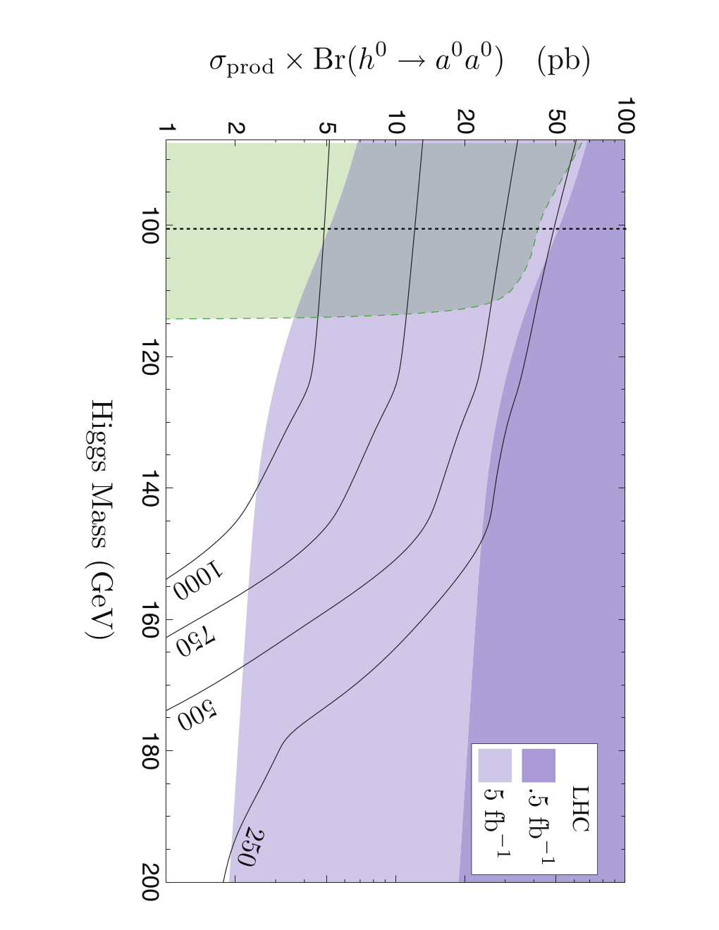
In comparison to the search, the signature is particularly challenging because the taus decay to leptons only a third of the time and the leptons are typically very soft [148]. Currently, there are several proposed searches for the signal at both ATLAS and CMS [150, 149]. The ATLAS collaboration is exploring the channel and CMS is looking at ()().
We have proposed an alternative search to that takes advantage of the pseudoscalar’s subdominant decay to muons [135]. In particular, we consider the case where one pseudoscalar decays to a pair of taus and the other decays to a pair of muons. This decay channel has not been previously explored because the decay into muons is suppressed by . For example, when GeV and , the branching fraction to taus is , while that into muons is . However, the Higgs production cross section can be large enough to compensate for this small branching fraction; the gluon-gluon fusion can be as high as 2 pb at the Tevatron or 50 pb at the LHC. It is therefore possible to get events at the Tevatron with 20 fb-1 and events at the LHC (at TeV) with 0.5 fb-1.
The signal topology for the search is as follows. The pseudoscalars are highly boosted and lead to nearly-collinear acoplanar lepton pairs. Each tau has a 66% hadronic branching fraction, so there is a 44% chance that both taus will decay to pions and neutrinos, which the detector will see as jets and missing energy. If only one tau decays hadronically, there will still be a jet and missing energy. About 3% of the time, both taus will decay to muons. The signal of interest is therefore
| (3.12) |
where refers to the ditau object. Because the taus are nearly collinear, they will often be picked out as a single jet. The missing energy is in the same direction as the jet.
To reduce the background contributions, all events are required to have a pair of oppositely-signed muons within , where each muon has a of at least 10 GeV. A jet veto of 15 and 50 GeV for Tevatron and LHC, respectively, is placed on all jets except the two hardest. Also, it is required that the hardest muon is separated from the by . The three higher level cuts are: , where is the sum of the transverse momentum of the two muons, , and . It is important to emphasize that standard lepton isolation must be altered when doing such searches. In particular, it is necessary to remove the adjacent muon’s track and energy before estimating the nearby hadronic activity.
The main backgrounds to this signal are: Drell-Yan muons recoiling against jets, electroweak processes, and leptons from hadronic resonances. The Drell-Yan background is the most important; in these events, the missing energy arises from jet energy mismeasurement or neutrinos from heavy semileptonic decays in jets. The Drell-Yan background dominates over electroweak contributions from WW and . Contributions to the hadronic backgrounds arise from several different sources. One example is the possibility of double semi-leptonic decays in jets (). This turns out to be minimal after cuts because high muons are rare and there is a lot of hadronic activity surrounding the muons. Another possibility comes from upsilon decays into taus, which then decay to muons. In this case, few events survive the cuts because the missing energy is in the direction of the muon pair and the spectrum of the upsilons falls off rapidly. The final possibility arises from leptonic decays of light mesons, such as the . This turns out to be minimal because high- muons only occur out on the Lorentzian tail of the decay width or on the Gaussian mismeasurement tail. In all, the hadronic contribution is of the Drell-Yan background. For a complete discussion of the backgrounds, see [135].
Figure 3.14 shows the 95% exclusion plot for the Tevatron and LHC for a pseudoscalar with GeV. For lighter pseudoscalars, the sensitivity can increase by a factor of two. The contour lines show the cross sections for values of . The search was recently done at DO using 4.2 fb-1 of data [136]. From the figure, it is clear that the Tevatron will start probing GeV with 10 fb-1 of data, and can probe up to 500 GeV when the projected 20 fb-1 luminosity is reached. The LHC will be able to recover the LEP limit with 1 fb-1 of data and has the potential for higgs discovery with a sub-fb-1 data set.
3.6 Determination of Higgs-Boson Couplings
M. Dührssen, M. Rauch, R. Lafaye, T. Plehn and D. Zerwas
After establishing the presence of a light Higgs boson at the LHC, the next step will be to measure its properties, in particular its couplings to other particles and to itself [152, 153, 109]. In the Standard Model these are completely determined by the measured masses of the particles together with the gauge coupling and the electroweak mixing angle. Deviations from these relations can occur through an extended Higgs sector such as the MSSM [5, 154, 155]. Another possibility for modifications are additional particles which can shift the couplings via loop contributions or lead to different branching ratios by providing additional decay channels.
We do not consider channels necessitating more than which should not feed back into the leading parameter set. Our underlying model for the analysis [153, 109] is the Standard Model where we let the Higgs couplings float freely around its Standard Model value. The main channels for the coupling measurements can be found in Refs. [157, 39, 40].
3.6.1 Determination
The study in [153] analyses the measurement of Higgs couplings in the mass range of to GeV. The errors are extracted as deviations on the coupling square. New invisible and/or undetectable Higgs boson decay modes are allowed. The channel is based on older analyses with higher sensitivities to this channel.
Figure 3.15 shows the precision on the coupling determination and the total width as function of the Higgs boson mass with and without systematic uncertainties for the combination of two LHC experiments at .

The crucial role of the bottom coupling for low Higgs masses is visible here, as the errors for all couplings are dominated by the large uncertainty on the measurement below the threshold mass. For these masses, errors range from -, above GeV a precision of - on is reached.
For the remainder of this short overview we will put the focus on a Higgs boson mass of GeV. This is the preferred region for a Standard Model Higgs boson from electroweak precision data and compatible with the lower limit from direct LEP searches [156]. The by far leading decay channel in this mass range is into a pair of bottom quarks. Via the total width it enters into the branching ratios of all other particles. Therefore a precise knowledge is essential, particularly in the light of the severely reduced -production-channel sensitivity which we now account for, and we include the recent subjet analysis [102]. It can greatly improve the accuracy on this coupling, up to similar levels than the older results, and is currently under study by both experimental groups [122]. Also now we do not allow for invisible or undetectable Higgs decay modes, so the total width is fixed to the sum of the observable Higgs decay widths. To perform the analysis we use the SFitter [158] framework to map these highly correlated measurements onto the parameter space. A detailed overview of the individual channels, its associated experimental and theory errors and the correlations between the errors is in Ref. [109].
We parametrize the Higgs couplings as deviations from its Standard Model value via
| (3.13) |
where the are independent of each other. Furthermore we allow for additional contributions to the two important loop-induced couplings and
| (3.14) |
where is the loop-induced coupling in the Standard Model, the contribution from modified tree-level couplings to Standard-Model particles, and an additional dimension-five contribution, for example from new heavy states. The relation to the definition in Fig. (3.15) is
| (3.15) |
Profile likelihood

| no effective couplings | with effective couplings | ratio | |||||||||
|---|---|---|---|---|---|---|---|---|---|---|---|
| RMS | RMS | ||||||||||
| — | — | — | |||||||||
| — | — | — | — | ||||||||
| — | — | — | — | ||||||||
In Fig. 3.16 we show profile likelihoods for various parameters, where we smear the set of data input arbitrarily within their respective errors. We see that in all cases a value of , i.e. the Standard Model solution, is compatible with the data. Furthermore for the tree-level couplings there are solutions at , corresponding to a flipped sign of the coupling. For the loop-induced couplings four solutions exist, originating from both unflipped and flipped sign for the coupling and the additional contribution to the effective coupling. In the case two solutions coincide at for exact data; due to the smearing they get shifted apart and we indeed see all possibilities distinctly. For the top-quark contribution is subleading, so all maxima are unique, but a pair of two, corresponding to flipped sign of the top-quark coupling, is close to each other and they get smeared into a single one.
Errors
In Tab. 3.1 we show the errors on the extraction of Higgs coupling parameters. We obtain these errors by running 10000 toy experiments and smearing the data around the true point including all experimental and theory errors. The best fits for each parameter we histogram and extract using a Gaussian fit of the central peak. As we do not expect the errors to be symmetric, we also fit a combination of two Gaussians with the same maximum and the same height, but different widths, labeling these () and (). We also show a root-mean-square (RMS) error. These are systematically higher as in this case outliers have larger impact.
In the left column we quote the errors for both additional contributions to the effective couplings set to zero and in the middle one when we also allow these couplings to deviate from zero. In the column on the right-hand side we show the errors on the ratio of the coupling to the coupling. We define them as the deviation from of the ratios of the coupling constants
| (3.16) |
We see immediately that the coupling obtains increased errors once we allow effective couplings due to its dominant contribution to . A similar effect we would expect for where the photon decay channel gets effectively removed but here the accuracy of the remaining measurements is sufficiently well. Both and couplings are strongly linked to , so here we do not see a change either.
In particular the coupling benefits from forming the ratio. This coupling appears in all rate predictions via the total width which leads to strong correlations. For all other couplings we observe minor improvements from the channels where the production-side enters the determination of the decay-side couplings.
3.6.2 Conclusions
In summary we can determine the Higgs couplings with an accuracy up to , and to about - in the phenomenologically favored region of GeV using an integrated luminosity of . Forming ratios of couplings can slightly improve these numbers. For a light Higgs boson the determination of its coupling to bottom quarks is crucial. Due to its large branching ratio it is linked to all channels via the total width. Therefore a reliable measurement for example using subjet analyses [102] is vital. Given these errors a distinction between the Standard Model and the MSSM or other decoupling models seems not likely, but dramatic modifications (like a gluophobic Higgs in the MSSM) will be clearly visible.
3.7 On the Possible Observation of Light Higgses at the LHC
D. Feldman, Z. Liu and P. Nath
The Higgs patterns in SUGRA models and the connection to the String Landscape are discussed.
3.7.1 Light Higgses in the SUGRA and String Landscape
An exhaustive survey of sparticle mass hierarchies and their signatures reveals the presence of light SUSY Higgses () in high scale models [56]. Such light Higgses have been uncovered in mSUGRA and non-universal SUGRA models, as well as in a class of D-brane models. The light Higgses are found to exist in specific mass hierarchies or Higgs Patterns (HPs) [56], and consist of SUGRA patterns labeled as mSP14, mSP15 and mSP16, which are defined by the following :
where a relative switch between the ordering of and the LSP () is possible as well. It is shown in [56] that these patterns are very stable with respect to nonuniversalities in the Higgs sector [160]. There are many other patterns that emerge in the survey of the SUGRA landscape. These may be classified minimally according to the NLSP, and there are found to be NLSPs which are the chargino, stau, stop, higgs, gluino and the sneutrino; comprising a total of around 40 4-particle mass patterns discounting the lightest CP even Higgs boson whose mass is fixed over a narrow corridor of about 25 GeV.


In fact the Higgs Patterns are found to be one of the more dominant patterns that can arise. These patterns are likely to be one of the first to be tested at the LHC, as we will discuss further.
Dark matter constraints on Higgs Patterns mSP(14-16)
The Higgs Patterns are found to be constrained by dark matter experiments from limits on the spin independent cross section, , as seen in Fig.(3.17). These constraints on the HPs arise specifically for low values of the neutralino mass. The for HPs is much larger than, for example, the stau pattern (SUP) mSP5. This is in part because of a larger Higgsino component of the LSP for the HPs relative to the Stau Pattern where the LSP is more bino like and also because the HPs have lighter neutral SUSY Higgs being exchanged for the same neutralino mass.
Discovering light Higgses at the LHC
The lightness of (and also of and ) in the HPs implies that the Higgs production cross sections at colliders can be enhanced for these patterns. This is especially true at large in processes via gluon fusion and bottom quark annihilations. Such an enhancement opens fruitful discovery prospects in the 2 mode as well as possibilities for the charged Higgs decaying into . For the case of large one is led to corroborating constraints from the recent Tevatron collider data including constraints on and, as already noted, from direct detection dark matter experiments [56]. In Fig.(3.18) we give a relative comparison of the effective mass distributions () of a single Higgs pattern (HP) and of a Chargino Pattern (CP) mSP1, a Stau Pattern (SUP) mSP5, and of a Stop Pattern (SOP) mSP11. The analysis of Fig.(3.18) shows that the HP and the SUP have a relatively larger while the of the CP and of SOP are much smaller. This is found more generally to be the case. The values of the effective mass are intimately tied to the length of the decay chains for the specific patterns and the overall scale of the colored sector. The fat distributions from the HPs make them easier to discover at the LHC, but can easily be confused with a SUP. Thus additional signatures are needed to discriminate among them. One such discriminating correlation of signatures is given in Fig.(3.18) which shows signals of the HPs vs other Patterns (CPs, SOPs, SUPs) in a plane of average missing vs. the fraction of events . Here one finds that the HPs and the SUPs are, on the whole, significantly well separated. In summary the analysis above illustrates that a combination of signatures at the LHC should give rise to the resolution of the Higgs Patterns from other SUSY patterns and allow one to discover the light Higgses of the HPs if such particles are indeed light.
Bibliography
- [1]
H. Nilles,
Phys. Rept. 110 (1984) 1;
H. Haber and G. Kane, Phys. Rept. 117 (1985) 75;
R. Barbieri, Riv. Nuovo Cim. 11 (1988) 1. - [2] S. Heinemeyer, W. Hollik and G. Weiglein, Phys. Rept. 425 (2006) 265 [arXiv:hep-ph/0412214].
- [3] S. Heinemeyer, Int. J. Mod. Phys. A 21 (2006) 2659 [arXiv:hep-ph/0407244].
- [4] A. Djouadi, Phys. Rept. 459 (2008) 1 [arXiv:hep-ph/0503173].
- [5] G. Degrassi, S. Heinemeyer, W. Hollik, P. Slavich and G. Weiglein, Eur. Phys. J. C 28 (2003) 133 [arXiv:hep-ph/0212020].
- [6] O. Buchmueller et al., to appear in Eur. Phys. J. C, arXiv:0907.5568 [hep-ph].
- [7] O. Buchmueller et al., Phys. Lett. B 657 (2007) 87 [arXiv:0707.3447 [hep-ph]].
- [8] O. Buchmueller et al., JHEP 0809 (2008) 117 [arXiv:0808.4128 [hep-ph]].
- [9]
http://lepewwg.web.cern.ch/
LEPEWWG/Welcome.html . - [10] R. Barate et al. [ALEPH, DELPHI, L3, OPAL Collaborations and LEP Working Group for Higgs boson searches], Phys. Lett. B 565 (2003) 61 [arXiv:hep-ex/0306033].
- [11] S. Schael et al. [ALEPH, DELPHI, L3, OPAL Collaborations and LEP Working Group for Higgs boson searches], Eur. Phys. J. C 47 (2006) 547 [arXiv:hep-ex/0602042].
- [12] J. R. Ellis, S. Heinemeyer, K. A. Olive and G. Weiglein, Phys. Lett. B 515 (2001) 348 [arXiv:hep-ph/0105061].
- [13] S. Ambrosanio, A. Dedes, S. Heinemeyer, S. Su and G. Weiglein, Nucl. Phys. B 624 (2002) 3 [arXiv:hep-ph/0106255].
- [14] G. L. Bayatian et al. [CMS Collaboration], J. Phys. G 34 (2007) 995.
- [15] S. Gennai, S. Heinemeyer, A. Kalinowski, R. Kinnunen, S. Lehti, A. Nikitenko and G. Weiglein, Eur. Phys. J. C 52 (2007) 383 [arXiv:0704.0619 [hep-ph]].
- [16] H. Georgi, S. Glashow, M. Machacek and D.V. Nanopoulos, Phys. Rev. Lett. 40 (1978) 692.
- [17] D. Graudenz, M. Spira and P.M. Zerwas, Phys. Rev. Lett. 70 (1993) 1372; M. Spira, A. Djouadi, D. Graudenz and P.M. Zerwas, Phys. Lett. B318 (1993) 347 and Nucl. Phys. B453 (1995) 17.
- [18] M. Krämer, E. Laenen and M. Spira, Nucl. Phys. B511 (1998) 523.
- [19] M. Spira, Fortsch. Phys. 46 (1998) 203.
- [20] A. Djouadi, Phys. Rept. 457 (2008) 1.
- [21] A. Djouadi, M. Spira and P.M. Zerwas, Phys. Lett. B264 (1991) 440;
- [22] S. Dawson, Nucl. Phys. B359 (1991) 283; R.P. Kauffman and W. Schaffer, Phys. Rev. D49 (1994) 551; S. Dawson and R.P. Kauffman, Phys. Rev. D49 (1994) 2298.
- [23] R.V. Harlander and W.B. Kilgore, Phys. Rev. Lett. 88 (2002) 201801 and JHEP 0210 (2002) 017; C. Anastasiou and K. Melnikov, Nucl. Phys. B646 (2002) 220; V. Ravindran, J. Smith and W.L. van Neerven, Nucl. Phys. B665 (2003) 325.
- [24] R. V. Harlander and K. J. Ozeren, arXiv:0907.2997 [hep-ph]; A. Pak, M. Rogal and M. Steinhauser, arXiv:0907.2998 [hep-ph].
- [25] S. Catani, D. de Florian, M. Grazzini and P. Nason, JHEP 0307 (2003) 028.
- [26] A. Djouadi, P. Gambino and B.A. Kniehl, Nucl. Phys. B523 (1998) 17;
- [27] A. Djouadi and P. Gambino, Phys. Rev. Lett. 73 (1994) 2528; K.G. Chetyrkin, B.A. Kniehl and M. Steinhauser, Phys. Rev. Lett. 78 (1997) 594 and Nucl. Phys. B490 (1997) 19; A. Ghinculov and J.J. van der Bij, Nucl. Phys. B482 (1996) 59; S. Actis, G. Passarino, C. Sturm and S. Uccirati, Phys. Lett. B 670 (2008) 12.
- [28] C. Anastasiou, R. Boughezal and F. Petriello, JHEP 0904 (2009) 003.
- [29] R. K. Ellis, I. Hinchliffe, M. Soldate and J. J. van der Bij, Nucl. Phys. B 297 (1988) 221.
- [30] U. Baur and E.W.N. Glover, Nucl. Phys. B339 (1990) 38.
- [31] C.R. Schmidt, Phys. Lett. B413 (1997) 391; D. de Florian, M. Grazzini and Z. Kunszt, Phys. Rev. Lett. 82 (1999) 5209; V. Ravindran, J. Smith and W.L. Van Neerven, Nucl. Phys. B634 (2002) 247; C.J. Glosser and C.R. Schmidt, JHEP 0212 (2002) 016; C. Anastasiou, K. Melnikov and F. Petriello, Nucl. Phys. B724 (2005) 197.
- [32] S. Catani, E. D’Emilio and L. Trentadue, Phys. Lett. B211 (1988) 335; I. Hinchliffe and S. Novaes, Phys. Rev. D38 (1988) 3475; R.P. Kauffman, Phys. Rev. D44 (1991) 1415 and Phys. Rev. D45 (1992) 1512; C. Balazs and C.P. Yuan, Phys. Lett. B478 (2000) 192; E.L. Berger and J.W. Qiu, Phys. Rev. D67 (2003) 034026; A. Kulesza and W.J. Stirling, JHEP 0312 (2003) 056; A. Kulesza, G. Sterman and W. Vogelsang, Phys. Rev. D69 (2004) 014012; A. Gawron and J. Kwiecinski, Phys. Rev. D70 (2004) 014003; G. Watt, A.D. Martin and M.G. Ryskin, Phys. Rev. D70 (2004) 014012 [Erratum-ibid. D70 (2004) 079902]; A.V. Lipatov and N.P. Zotov, Eur. Phys. J. C44 (2005) 559.
- [33] D. de Florian and M. Grazzini, Phys. Rev. Lett. 85 (2000) 4678 and Nucl. Phys. B616 (2001) 247; S. Catani, D. de Florian and M. Grazzini, Nucl. Phys. B596 (2001) 299; G. Bozzi, S. Catani, D. de Florian and M. Grazzini, Phys. Lett. B564 (2003) 65; G. Bozzi, S. Catani, D. de Florian and M. Grazzini, Nucl. Phys. B 737 (2006) 73 and Nucl. Phys. B 791 (2008) 1.
- [34] V. Del Duca, W. Kilgore, C. Oleari, C. Schmidt and D. Zeppenfeld, Nucl. Phys. B 616, 367 (2001) [arXiv:hep-ph/0108030].
- [35] S. Dawson and R. P. Kauffman, Phys. Rev. Lett. 68, 2273 (1992); R. P. Kauffman, S. V. Desai and D. Risal, Phys. Rev. D 55, 4005 (1997) [Erratum-ibid. D 58, 119901 (1998)] [arXiv:hep-ph/9610541].
- [36] J. M. Campbell, R. K. Ellis and G. Zanderighi, JHEP 0610, 028 (2006) [arXiv:hep-ph/0608194].
- [37] R.N. Cahn and S. Dawson, Phys. Lett. B136 (1984) 196; K. Hikasa, Phys. Lett. B164 (1985) 341; G. Altarelli, B. Mele and F. Pitolli, Nucl. Phys. B287 (1987) 205.
- [38] T. Han, G. Valencia and S. Willenbrock, Phys. Rev. Lett. 69 (1992) 3274.
- [39] T. Figy, C. Oleari and D. Zeppenfeld, Phys. Rev. D68 (2003) 073005; E.L. Berger and J. Campbell, Phys. Rev. D70 (2004) 073011.
- [40] M. Ciccolini, A. Denner and S. Dittmaier, Phys. Rev. D 77 (2008) 013002.
- [41] S.L. Glashow, D.V. Nanopoulos and A. Yildiz, Phys. Rev. D18 (1978) 1724; Z. Kunszt, Z. Trocsanyi and W.J. Stirling, Phys. Lett. B271 (1991) 247.
- [42] T. Han and S. Willenbrock, Phys. Lett. B273 (1991) 167.
- [43] O. Brein, A. Djouadi and R. Harlander, Phys. Lett. B579 (2004) 149.
- [44] M.L. Ciccolini, S. Dittmaier and M. Krämer, Phys. Rev. D68 (2003) 073003.
- [45] R. Raitio and W.W. Wada, Phys. Rev. D19 (1979) 941; J.N. Ng and P. Zakarauskas, Phys. Rev. D29 (1984) 876; Z. Kunszt, Nucl. Phys. B247 (1984) 339; J.F. Gunion, Phys. Lett. B253 (1991) 269; W.J. Marciano and F.E. Paige, Phys. Rev. Lett. 66 (1991) 2433.
- [46] W. Beenakker, S. Dittmaier, M. Krämer, B. Plümper, M. Spira and P.M. Zerwas, Phys. Rev. Lett. 87 (2001) 201805 and Nucl. Phys. B653 (2003) 151; S. Dawson, L.H. Orr, L. Reina and D. Wackeroth, Phys. Rev. D67 (2003) 071503.
- [47] S. Dawson and L. Reina, Phys. Rev. D57 (1998) 5851.
- [48] M. Mühlleitner and M. Spira, Nucl. Phys. B 790 (2008) 1;
- [49] S. Dawson, A. Djouadi and M. Spira, Phys. Rev. Lett. 77 (1996) 16; R. Bonciani, G. Degrassi and A. Vicini, JHEP 0711 (2007) 095; M. Mühlleitner, H. Rzehak and M. Spira, JHEP 0904 (2009) 023.
- [50] G. Degrassi and P. Slavich, Nucl. Phys. B 805 (2008) 267;
- [51] C. Anastasiou, S. Beerli and A. Daleo, Phys. Rev. Lett. 100 (2008) 241806.
- [52] R.V. Harlander and M. Steinhauser, Phys. Lett. B574 (2003) 258, Phys. Rev. D68 (2003) 111701, JHEP 0409 (2004) 066; R.V. Harlander and F. Hofmann, JHEP 0603 (2006) 050;
- [53] U. Langenegger, M. Spira, A. Starodumov and P. Trüb, JHEP 0606 (2006) 035; O. Brein and W. Hollik, Phys. Rev. D 68 (2003) 095006.
- [54] T. Plehn, D. L. Rainwater and D. Zeppenfeld, Phys. Lett. B 454 (1999) 297 [arXiv:hep-ph/9902434];
- [55] A. Djouadi and M. Spira, Phys. Rev. D62 (2000) 014004; W. Hollik, T. Plehn, M. Rauch and H. Rzehak, Phys. Rev. Lett. 102 (2009) 091802.
- [56] W. Peng, M. Wen-Gan, H. Hong-Sheng, Z. Ren-You, H. Liang and J. Yi, arXiv:hep-ph/0505086; W. Hollik and M. Rauch, AIP Conf. Proc. 903 (2007) 117; P. Häfliger, PhD thesis ETH Zürich 2006, DISS-ETH-16970; M. Walser, “ PhD thesis ETH Zürich 2008, DISS-ETH-17592; S. Dittmaier, P. Häfliger, M. Krämer, M. Spira and M. Walser, in preparation.
- [57] S. Dittmaier, M. Krämer and M. Spira, Phys. Rev. D70 (2004) 074010; S. Dawson, C.B. Jackson, L. Reina and D. Wackeroth, Phys. Rev. D69 (2004) 074027.
- [58] D.A. Dicus and S. Willenbrock, Phys. Rev. D39 (1989) 751.
- [59] D. Dicus, T. Stelzer, Z. Sullivan and S. Willenbrock, Phys. Rev. D59 (1999) 094016; C. Balazs, H.J. He and C.P. Yuan, Phys. Rev. D60 (1999) 114001.
- [60] R.V. Harlander and W.B. Kilgore, Phys. Rev. D68 (2003) 013001.
- [61] H. Eberl, K. Hidaka, S. Kraml, W. Majerotto and Y. Yamada, Phys. Rev. D62 (2000) 055006;
- [62] J. A. Coarasa, R.A. Jimenez and J. Solà, Phys. Lett. B389 (1996) 312;
- [63] J. Guasch, P. Häfliger and M. Spira, Phys. Rev. D68 (2003) 115001.
- [64] S. Dittmaier, M. Krämer, A. Mück and T. Schlüter, JHEP 0703 (2007) 114.
- [65] J. Campbell et al., arXiv:hep-ph/0405302.
- [66] J. Campbell, R.K. Ellis, F. Maltoni and S. Willenbrock, Phys. Rev. D67 (2003) 095002; S. Dawson, C.B. Jackson, L. Reina and D. Wackeroth, Phys. Rev. Lett. 94 (2005) 031802.
- [67] A.C. Bawa, C.S. Kim and A.D. Martin, Z. Phys. C47 (1990) 75; F. Borzumati, J.L. Kneur and N. Polonsky, Phys. Rev. D60 (1999) 115011; A. Belyaev, D. Garcia, J. Guasch and J. Sola, JHEP 0206 (2002) 059.
- [68] S. Dittmaier, M. Krämer, M. Spira and M. Walser, arXiv:0906.2648 [hep-ph].
- [69] W. Peng, M. Wen-Gan, Z. Ren-You, J. Yi, H. Liang and G. Lei, Phys. Rev. D73 (2006) 015012.
- [70] S.H. Zhu, Phys. Rev. D67 (2003) 075006; T. Plehn, Phys. Rev. D67 (2003) 014018; E.L. Berger, T. Han, J. Jiang and T. Plehn, Phys. Rev. D71 (2005) 115012; G.P. Gao, G.R. Lu, Z.H. Xiong and J.M. Yang, Phys. Rev. D66 (2002) 015007.
- [71] S. Willenbrock, Phys. Rev. D35 (1987) 173; A. Krause, T. Plehn, M. Spira and P.M. Zerwas, Nucl. Phys. B519 (1998) 85; Y. Jiang, L. Han, W.G. Ma, Z.H. Yu and M. Han, J. Phys. G23 (1997) 385 [Erratum-ibid. G23 (1997) 1151]; O. Brein and W. Hollik, Eur. Phys. J. C13 (2000) 175.
- [72] A.A. Barrientos Bendezu and B.A. Kniehl, Nucl. Phys. B568 (2000) 305.
- [73] H. Hong-Sheng, M. Wen-Gan, Z. Ren-You, J. Yi, H. Liang and X. Li-Rong, Phys. Rev. D71 (2005) 075014.
- [74] A.A. Barrientos Bendezu and B.A. Kniehl, Phys. Rev. D59 (1999) 015009; O. Brein, W. Hollik and S. Kanemura, Phys. Rev. D63 (2001) 095001.
- [75] A.A. Barrientos Bendezu and B.A. Kniehl, Phys. Rev. D 63 (2001) 015009.
- [76] D.A. Dicus, J.L. Hewett, C. Kao and T.G. Rizzo, Phys. Rev. D 40 (1989) 787;
- [77] W. Hollik and S.H. Zhu, Phys. Rev. D65 (2002) 075015; J. Zhao, C.S. Li and Q. Li, Phys. Rev. D72 (2005) 114008.
- [78] E. Braaten and J.P. Leveille, Phys. Rev. D22 (1980) 715; N. Sakai, Phys. Rev. D22 (1980) 2220; T. Inami and T. Kubota, Nucl. Phys. B179 (1981) 171; S.G. Gorishny, A.L. Kataev, S.A. Larin and L.R. Surguladze, Mod. Phys. Lett. A5 (1990) 2703; Phys. Rev. D43 (1991) 1633; M. Drees and K. Hikasa, Phys. Lett. B240 (1990) 455 and (E) B262 (1991) 497; A.L. Kataev and V.T. Kim, Mod. Phys. Lett. A9 (1994) 1309; K.G. Chetyrkin, J.H. Kühn and A. Kwiatkowski, Proceedings of the Workshop “QCD at LEP”, Aachen 1994; K.G. Chetyrkin and A. Kwiatkowski, Report LBL-37269; A. Djouadi and P. Gambino, Phys. Rev. D51 (1995) 218; K.G. Chetyrkin, Phys. Lett. B390 (1997) 309.
- [79] J. Fleischer and F. Jegerlehner, Phys. Rev. D23 (1981) 2001; D.Yu. Bardin, B.M. Vilenskiǐ and P.Kh. Khristova, Sov. J. Nucl. Phys. 53 (1991) 152; A. Dabelstein and W. Hollik, Z. Phys. C53 (1992) 507; B.A. Kniehl, Nucl. Phys. B376 (1992) 3.
- [80] B.A. Kniehl, Nucl. Phys. B352 (1991) 1 and B357 (1991) 357; D.Yu. Bardin, B.M. Vilenskiǐ and P.Kh. Khristova, Report JINR-P2-91-140.
- [81] T.G. Rizzo, Phys. Rev. D22 (1980) 389; W.-Y. Keung and W.J. Marciano, Phys. Rev. D30 (1984) 248.
- [82] A Bredenstein, A. Denner, S. Dittmaier and M.M. Weber, JHEP0702 (2007) 080.
- [83] M. Spira, A. Djouadi, D. Graudenz and P.M. Zerwas, Nucl. Phys. B453 (1995) 17.
- [84] K.G. Chetyrkin, B.A. Kniehl and M. Steinhauser, Phys. Rev. Lett. 79 (1997) 353; M. Steinhauser, Phys. Rept. bf 364 (2002) 247; M. Schreck and M. Steinhauser, Phys. Lett. B655 (2007) 148.
- [85] P.A. Baikov and K.G. Chetyrkin, Phys. Rev. Lett. 97 (2006) 061803.
- [86] H. Zheng and D. Wu, Phys. Rev. D42 (1990) 3760; A. Djouadi, M. Spira, J. van der Bij and P.M. Zerwas, Phys. Lett. B257 (1991) 187; S. Dawson and R.P. Kauffman, Phys. Rev. D47 (1993) 1264; A. Djouadi, M. Spira and P.M. Zerwas, Phys. Lett. B311 (1993) 255; K. Melnikov and O. Yakovlev, Phys. Lett. B312 (1993) 179; M. Inoue, R. Najima, T. Oka and J. Saito, Mod. Phys. Lett. A9 (1994) 1189; M. Steinhauser, hep-ph/9612395.
- [87] U. Aglietti, R. Bonciani, G. Degrassi and A. Vicini, Phys. Lett. B595 (2004) 432; F. Fugel, B.A. Kniehl and M. Steinhauser, Nucl. Phys. B702 (2004) 333; G. Degrassi and F. Maltoni, Nucl. Phys. B724 (2005) 183; G. Passarino, C. Sturm and S. Uccirati, Phys. Lett. B655 (2007) 298.
- [88] A. Djouadi, J. Kalinowski and M. Spira, Comput. Phys. Commun. 108 (1998) 56 [arXiv:hep-ph/9704448];
- [89] A. Dabelstein, Nucl. Phys. B456 (1995) 25.
- [90] S. Heinemeyer, W. Hollik and G. Weiglein, Eur. Phys. J. C16 (2000) 139.
- [91] M. Carena, D. Garcia, U. Nierste and C.E.M. Wagner, Nucl. Phys. B577 (2000) 88;
- [92] D. Noth and M. Spira, Phys. Rev. Lett. 101 (2008) 181801.
- [93] U. Aglietti, R. Bonciani, G. Degrassi and A. Vicini, JHEP0701 (2007) 021;
- [94] A. Djouadi, P. Janot, J. Kalinowski and P.M. Zerwas, Phys. Lett. B376 (1996) 220; A. Djouadi, J. Kalinowski, P. Ohmann and P.M. Zerwas, Z. Phys. C74 (1997) 93; A. Bartl, H. Eberl, K. Hidaka, T. Kon, W. Majerotto and Y. Yamada, Phys. Lett. B389 (1996) 538.
- [95] F. Boudjema and E. Chopin, Z. Phys. C73 (1996) 85; P. Osland and P.N. Pandita, Phys. Rev. D59 (1999) 055013; A. Djouadi, W. Kilian, M. Mühlleitner and P.M. Zerwas, Eur. Phys. J. C10 (1999) 45; A. Djouadi, W. Kilian, M. Mühlleitner and P.M. Zerwas, Eur. Phys. J. C10 (1999) 27.
- [96] W. Hollik and S. Penaranda, Eur. Phys. J. C23 (2002) 163; A. Dobado, M.J. Herrero, W. Hollik and S. Penaranda, Phys. Rev. D66 (2002) 095016.
- [97] Atlas Collaboration,CERN-LHCC-99-15.
- [98] V. Buescher and K. Jakobs, Int. J. Mod. Phys. A 20 (2005) 2523 [arXiv:hep-ph/0504099]; D. Rainwater, arXiv:hep-ph/0702124.
- [99] CMS Collaboration, CMS PAS HIG-008-003.
- [100] G. Aad et al. [The ATLAS Collaboration], arXiv:0901.0512 [hep-ex].
- [101] M. Dittmar and H. K. Dreiner, Phys. Rev. D 55 (1997) 167 [arXiv:hep-ph/9608317].
- [102] T. Binoth, M. Ciccolini, N. Kauer and M. Kramer, JHEP 0612 (2006) 046 [arXiv:hep-ph/0611170].
- [103] N. Kauer, T. Plehn, D. L. Rainwater and D. Zeppenfeld, Phys. Lett. B 503 (2001) 113 [arXiv:hep-ph/0012351].
- [104] T. Plehn, D. L. Rainwater and D. Zeppenfeld, Phys. Rev. D 61 (2000) 093005 [arXiv:hep-ph/9911385].
- [105] K. Cranmer and T. Plehn, Eur. Phys. J. C 51 (2007) 415 [arXiv:hep-ph/0605268].
- [106] S. Dawson, S. Dittmaier and M. Spira, Phys. Rev. D 58 (1998) 115012 [arXiv:hep-ph/9805244].
- [107] U. Baur, T. Plehn and D. L. Rainwater, Phys. Rev. Lett. 89 (2002) 151801 [arXiv:hep-ph/0206024].
- [108] A. Djouadi, M. M. Muhlleitner and M. Spira, Acta Phys. Polon. B 38 (2007) 635 [arXiv:hep-ph/0609292].
- [109] R. Lafaye, T. Plehn, M. Rauch, D. Zerwas and M. Duhrssen, JHEP 0908 (2009) 009, [arXiv:0904.3866 [hep-ph]].
- [110] D. L. Rainwater and D. Zeppenfeld, Phys. Rev. D 60 (1999) 113004 [Erratum-ibid. D 61 (2000) 099901] [arXiv:hep-ph/9906218].
- [111] A. J. Barr, B. Gripaios and C. G. Lester, JHEP 0907 (2009) 072 [arXiv:0902.4864 [hep-ph]].
- [112] K. Choi, S. Choi, J. S. Lee and C. B. Park, arXiv:0908.0079 [hep-ph].
- [113] C. Anastasiou, G. Dissertori, M. Grazzini, F. Stockli and B. R. Webber, JHEP 0908 (2009) 099 [arXiv:0905.3529 [hep-ph]].
- [114] W. Y. Keung and F. J. Petriello, Phys. Rev. D 80 (2009) 013007 [arXiv:0905.2775 [hep-ph]].
- [115] D. de Florian and M. Grazzini, Phys. Lett. B674 (2009) 291 [arXiv:0901.2427[hep-ph]].
- [116] S. Frixione and B. R. Webber, arXiv:hep-ph/0207182.
- [117] S. Frixione, P. Nason and C. Oleari, JHEP 0711 (2007) 070 [arXiv:0709.2092 [hep-ph]].
- [118] S. Catani, F. Krauss, R. Kuhn and B. R. Webber, JHEP 0111 (2001) 063 [arXiv:hep-ph/0109231].
- [119] M. L. Mangano, M. Moretti and R. Pittau, Nucl. Phys. B 632 (2002) 343 [arXiv:hep-ph/0108069].
- [120] J. M. Butterworth, A. R. Davison, M. Rubin and G. P. Salam, Phys. Rev. Lett. 100 (2008) 242001 [arXiv:0802.2470 [hep-ph]].
- [121] for an alternative approach see e.g. S. D. Ellis, C. K. Vermilion and J. R. Walsh, arXiv:0903.5081 [hep-ph].
- [122] The ATLAS collaboration, ATL-PHYS-PUB-2009-088.
- [123] T. Plehn, G. Salam and M. Spannowsky, arXiv:0910.5472 [hep-ph].
- [124] A. Bredenstein, A. Denner, S. Dittmaier and S. Pozzorini, Phys. Rev. Lett. 103 (2009) 012002 [arXiv:0905.0110 [hep-ph]], G. Bevilacqua, M. Czakon, C. G. Papadopoulos, R. Pittau and M. Worek, JHEP 0909 (2009) 109 [arXiv:0907.4723 [hep-ph]].
- [125] R. Dermisek and J. F. Gunion, Phys. Rev. Lett. 95 (2005) 041801 [arXiv:hep-ph/0502105].
- [126] R. E. Shrock and M. Suzuki, Phys. Lett. B 110 (1982) 250.
- [127] J. F. Gunion, H. E. Haber and T. Moroi, [arXiv:hep-ph/9610337].
- [128] S. Chang, R. Dermisek, J. F. Gunion and N. Weiner, Ann. Rev. Nucl. Part. Sci. 58 (2008) 75 [arXiv:0801.4554 [hep-ph]].
- [129] S. Chang and T. Gregoire, arXiv:0903.0403 [hep-ph].
- [130] B. Bellazzini, C. Csaki, A. Falkowski and A. Weiler, arXiv:0906.3026 [hep-ph].
- [131] M. Carena, T. Han, G. Y. Huang and C. E. M. Wagner, JHEP 0804 (2008) 092 [arXiv:0712.2466 [hep-ph]].
- [132] M. J. Strassler and K. M. Zurek, Phys. Lett. B 661, 263 (2008) [arXiv:hep-ph/0605193].
- [133] V. M. Abazov et al. [D0 Collaboration], Phys. Rev. Lett. 103 (2009) 071801 [arXiv:0906.1787 [hep-ex]].
- [134] D. E. Kaplan and M. McEvoy, arXiv:0909.1521 [hep-ph].
- [135] M. Lisanti and J. G. Wacker, Phys. Rev. D 79 (2009) 115006 [arXiv:0903.1377 [hep-ph]].
- [136] V. M. Abazov et al. [D0 Collaboration], Phys. Rev. Lett. 103 (2009) 061801 [arXiv:0905.3381 [hep-ex]].
- [137] G. Hiller, Phys. Rev. D 70 (2004) 034018 [arXiv:hep-ph/0404220].
- [138] B. Aubert et al. [BABAR Collaboration], arXiv:0906.2219 [hep-ex].
- [139] B. Aubert et al. [BABAR Collaboration], Phys. Rev. Lett. 103 (2009) 081803 [arXiv:0905.4539 [hep-ex]].
- [140] R. Dermisek, J. F. Gunion and B. McElrath, Phys. Rev. D 76 (2007) 051105 [arXiv:hep-ph/0612031].
- [141] T. C. Collaboration, t. D. Collaboration, t. T. N. Physics and H. W. Group, arXiv:0911.3930 [hep-ex].
- [142] LEP-EWWG, http://www.cern.ch/LEPEWWG.
- [143] G. Abbiendi et al. [OPAL Collaboration], Eur. Phys. J. C 27, 311 (2003) [arXiv:hep-ex/0206022].
- [144] G. Abbiendi et al. [OPAL Collaboration], Eur. Phys. J. C 27, 483 (2003) [arXiv:hep-ex/0209068].
- [145] G. Abbiendi et al. [OPAL Collaboration], Eur. Phys. J. C 37, 49 (2004) [arXiv:hep-ex/0406057].
- [146] J. Abdallah et al. [DELPHI Collaboration], Eur. Phys. J. C 38, 1 (2004) [arXiv:hep-ex/0410017].
- [147] K. m. Cheung, J. Song and Q. S. Yan, arXiv:0710.1997 [hep-ph].
- [148] P. W. Graham, A. Pierce and J. G. Wacker, arXiv:hep-ph/0605162.
- [149] N. E. Adam et al., arXiv:0803.1154 [hep-ph].
- [150] J. R. Forshaw, J. F. Gunion, L. Hodgkinson, A. Papaefstathiou and A. D. Pilkington, JHEP 0804, 090 (2008) [arXiv:0712.3510 [hep-ph]].
- [151] K. Cranmer, ”Searching for Exotic Higgs Decays at LEP.” Presentation at the Conference on the Search for New States and Forces of Nature at the Galileo Galilei Institute for Theoretical Physics, October 2009.
- [152] D. Zeppenfeld, R. Kinnunen, A. Nikitenko and E. Richter-Was, Phys. Rev. D 62 (2000) 013009 ; C. P. Burgess, J. Matias and M. Pospelov, Int. J. Mod. Phys. A 17 (2002) 1841.
- [153] M. Dührssen, S. Heinemeyer, H. Logan, D. Rainwater, G. Weiglein and D. Zeppenfeld, Phys. Rev. D 70 (2004) 113009 ;
- [154] for a pedagogical introduction see e.g. S. P. Martin, arXiv:hep-ph/9709356; I. J. R. Aitchison, arXiv:hep-ph/0505105; J. F. Gunion and H. E. Haber, Phys. Rev. D 67 (2003) 075019 .
- [155] H. E. Haber, R. Hempfling and A. H. Hoang, Z. Phys. C 75 (1997) 539 ; T. Hahn, S. Heinemeyer, W. Hollik, H. Rzehak, G. Weiglein and K. Williams, Pramana 69 (2007) 861 .
- [156] [ALEPH Collaboration and CDF Collaboration and D0 Collaboration and an], arXiv:0811.4682 [hep-ex].
- [157] M. Dührssen, ATL-PHYS-2003-030.
- [158] R. Lafaye, T. Plehn, M. Rauch and D. Zerwas, Eur. Phys. J. C 54 (2008) 617 [arXiv:0709.3985 [hep-ph]].
- [159] D. Feldman, Z. Liu , P. Nath, Phys. Rev. Lett. 99, 251802 (2007); Phys. Lett. B 662, 190 (2008); JHEP 0804, 054 (2008); AIP Conf. Proc. 1078, 116 (2009); Phys. Rev. D 80, 015007 (2009).
- [160] P. Nath, R. L. Arnowitt, Phys. Rev. D 56 (1997) 2820; J. R. Ellis, K. A. Olive, Y. Santoso, Phys. Lett. B 539 (2002) 107.
Chapter 4 CP Violation at the LHC
20
We give a brief overview of the hunt for CP violation in supersymmetric signatures at the LHC. Such signatures could arise from large CP violating phases which are still consistent with the electric dipole moment (EDM) experiments for the EDMs of the electron, for the neutron and for the Mercury and Thallium atoms. Specifically reviewed are the potential signatures that arise from a supersymmetric CP-violating Higgs sector at the LHC. As particular examples, we discuss phenomena of Higgs-sector CP violation at the LHC based on the MSSM scenarios CPX and Trimixing. Also discussed are the possible tests of the Cancelation Mechanism from various processes such as from studies of CP violating effects on , and CP effects on sparticle decays as well effects on dark matter which is strongly interconnected with LHC physics in supersymmetric unified models of particle interactions.
4.1 CP violation in Supersymmmetric Theories
The Standard Model of particle interactions has two sources of CP violation, one that enters in the Cabibbo-Kobayashi-Maskawa (CKM) matrix () and the other that enters in the strong interaction dynamics via the term , where is the gluonic field strength. These phases are constrained by the neutron electric dipole moment (EDM) so that . The phase that enters in the CKM matrix is also separately constrained, for example, by the condition
| (4.1) |
This constraint can be exhibited by a unitarity triangle with angles where , , and . Our current direct knowledge of CP violation hinges on experiments on the K and B systems. This evidence arises in the neutral Kaon system in the form of and where experimentally
| (4.2) |
In the B system () decay gives a direct measurement of so that
| (4.3) |
Finally another piece of evidence for CP violation comes from the baryon asymmetry in the universe so that
| (4.4) |
The experimental results of Eqs. (4.2) and Eq. (4.3) are consistent with CP violation given by the Standard Model. However, an explanation of the baryon asymmetry in the universe implies the need of a CP violation beyond the Standard Model. Further, it is possible that in the future more accurate measurements of the angles may indicate a breakdown of the unitarity triangle which would point to the existence of a source of CP violation beyond the standard model. Another possible indication of a new source of CP violation would be an experimental observation of an EDM of elementary fermions. Specifically in the Standard Model the EDM of a lepton arises at the multiloop level [1] and is too small to be observed (see Table 4.1). However, much larger EDMs can arise in supersymmetric theories.
| Table 1: Lepton EDMs | ||
|---|---|---|
| SM (ecm) | Experiment (ecm) | |
Thus softly broken supersymmtric theories contain additional sources of CP violation. For example, in mSUGRA with the inclusion of CP phases , and become complex. However, one of these phases can be rotated away and one may choose the remaining complex parameters to be and so that and . So in this case the complex mSUGRA model (cmSUGRA) has the following parameter space
| (4.5) |
Such new sources of CP violation may play a role in the generation of a baryon asymmetry in the universe. However, the new CP phases are constrained by the experimental limits on the EDMs of the electron, of the neutron, and of atoms such as of Hg, and Thallium. In non-universal SUGRA models one can get a much larger set of phases. Thus, e.g., allowing for arbitrary masses () for the gauginos and for the trilinear couplings () one has
| (4.6) |
However, as mentioned earlier not all the phases are independent and further in physical computations only certain combinations appear as exhibited in Table (2).


As mentioned above the current data on the EDM of the electron, of the neutron and of the atoms impose rather severe contraints. The electron and the quarks receive contributions from the electric dipole operator (see Eq. (4.7)) and Fig. (4.1)) while the quarks receive contributions to their EDMs from the electric dipole operator, the chromoelectric dipole operator (see Eq. (4.8), and from the purely gluonic dimension six operator of Weinberg (see Eq. (4.9)) and the right panel of Fig. (4.1)).
| (4.7) |
| (4.8) |
| (4.9) |
where is the gluon field strength tensor, are the Gell-Mann coefficients, and is the totally antisymmetric tensor with . In addition, there are important two loop contributions to the EDMs as shown in Fig. (4.2).


As mentioned earlier not all the phases are independent and thus
the phases enter the EDMs of the leptons and of the quarks only in certain combinations
which are shown in Table (2).
CP phases also arise in string models. Recently there has been considerable progress,
for example, in constructing models based on M theory compactified on CY
and models in the framework of Type IIB orientifolds. Thus in compactifications on a Type IIB
theory on a six-torus , CP violation will arise in F-type breaking which may
be parametrized by
| (4.10) |
where S is the dilaton field, and the moduli fields, and parametrize
the Goldstino direction in the field space and . Here one
has four CP violating phases ().
However,
one problem encountered both in MSSM and in string based models
is the so called supersymmetric CP problem, i.e., that the
phases arising from the soft parameters give too large an EDM for the electron and for
the quarks. Several ways have been suggested to control this problem. One solution
is that CP phases are small [5]. This requires a rather artificial fine tuning of phases since
in most supersymmetric models and in string models the CP phases are
typically not suppressed. Another proposal is that the phases could be but their
contributions are suppressed due to heavy sparticle masses [6]. However, from the point
of view of discovery of the sparticles very heavy masses are not preferred. One possibility
which allows for large phases consistent with a light sparticle spectrum is the so called
cancellation mechanism proposed in[7] (For further work see [8, 9]).
Here one finds that contributions to the EDMs
from different sources tend to cancel each other with an appropriate choice of phases.
Thus, e.g., cancellations can occur in the EDM of the electron between contributions from
the chargino and from the neutralinos. For the EDMs of the quarks there can be additionally
cancellations between the contributions arising from the electric dipole, chromoelectric dipole
and the purely gluonic dimension six operator. As a consequence of these cancellations
it is possible to have large CP phases and compatibilty with the experimental EDM data.
Finally, it is possible that by some symmetry principle phases in the first two generations
vanish or are highly suppressed and CP phases arise only in the third generation. In this
case the EDMs will also be suppressed but the CP phases in the third generation could be
large. For another possible solution to the SUSY CP problem see [10].

The EDMs of the quarks and of the leptons are of course very sensitive to the phases as they arise directly from the phases. It is interesting, however, that the anomlaous magnetic moments of quarks and of leptons are also sensitive to the phases. In Fig. (4.4) we give a display of the sensitivity of the supersymmetric contribution to the anomalous magnetic moment of the muon on the phases. One finds that the CP phases can change both the sign and the magnitude of the supersymmetric contribution. It is then reasonable to ask if the current experimental data on the muon anomalous moment puts constraints on the allowed parameter space of the CP violating phases. An analysis of this issue shows that this indeed is the case. As an illustration the constraints arising from the Brookhaven experiment on and are shown in Fig. (4.5). One finds that indeed the Brookhaven experiment on puts severe constraints on the allowed region of the CP phases for a given set of other soft parameters eliminating large parts of the parameter space as exhibited in Fig. (4.5).


If the CP phases are large then many physical processes, some of them directly measurable at the LHC, will be affected and consequently a discovery of such phases can come about at the LHC. Thus the phases appear in a number of processes such as in the decay [13], in the production and decay of the sparticles [14, 15, 16], and in neutralino relic density analyses and in the direct detection of neutralino dark matter [50, 18]. Further, large CP phases from the soft parameters produce through one loop effective potential induced CP violating phases in the Higgs sector allowing for a mixing between the CP even and CP odd Higgs neutral Higgs fields. Such mixing effects can be discerned in the LHC data. This topic is discussed in further detail below.
| Table 2: Examples of CP phases in SUSY phenomena | |
|---|---|
| SUSY Quantity | Combinations of CP violating phases |
| () | (, ) |
| , , , | |
| ,.. | , ,, ,. |
| ,.. | , , , ,. |
| , , | |
| (small ) | |
| (large ) | , , , |
| , , , | |
| () | , , ( ) |
| , , , | |
| , | |
4.2 CP violation in the Higgs sector
As discussed already the Standard Model (SM) has two sources of CP violation: the Kobayashi–Maskawa (KM) phase in the quark mixing matrix and the so-called strong CP phase through the QCD anomaly. The Higgs potential of the Standard Model is CP-invariant to all orders, whereas a possible mixing of the boson with the SM Higgs boson can first occur at the 3-loop level [19] and is therefore very suppressed. Significant new sources of CP violation emerge in minimal Higgs-sector extensions of the SM, such as the two Higgs-doublet model [20].
A very predictive model with an extended Higgs sector and new sources of CP violation is the Minimal Supersymmetric Standard Model (MSSM), with supersymmetry (SUSY) softly broken at the TeV scale. In the MSSM, assuming flavour conservation, there are 12 physical combinations of CP phases [21, 22] 11 1 The relevant soft-SUSY breaking terms are as in
| (4.11) |
with and . In the convention of real and positive and , the most relevant CP phases pertinent to the Higgs sector are
| (4.12) |
with .
The Higgs sector of the MSSM consists of two doublets:
The neutral components can be rewritten in terms of 4 real field as
| (4.18) |
where and are CP-even and CP-odd fields, respectively. After the electroweak symmetry breaking, and , we are left with 5 Higgs states: 2 charged and 3 neutral. The 3 neutral states consists of one CP-odd state, , and two CP-even ones, and . At the tree level, the Higgs potential is CP invariant and the mixing between the two CP-even states is described by the matrix with the mixing angle as
| (4.19) |
However, the presence of the soft CP phases may introduce sizeable CP-violating couplings in the MSSM Higgs potential through radiative corrections [19, 23]. In particular, the non-vanishing CP phases of third generation terms could radiatively induce significant mixing between the CP-even and CP-odd states proportional to [19, 23, 24, 25, 26, 27, 28, 29, 30]
| (4.20) |
The CP phase of the gluino mass parameter also contribute to the CP-violating Higgs mixing through the so-called threshold corrections to the Yukawa couplings
| (4.21) |
where
| (4.22) | |||||
with
| (4.23) |
This is formally a two-loop effect but could be important when is large.
The consequences of the CP-violating mixing among the three neutral Higgs bosons are: the neutral Higgs bosons do not have to carry any definite CP parities, the neutral Higgs-boson mixing is described by the mixing matrix as with the lightest (heaviest) Higgs state, the couplings of the Higgs bosons to the SM and SUSY particles are significantly modified. In our numerical analysis, we use the code CPsuperH [31, 32] which is based on the renormalization-group-(RG-)improved effective potential approach.
4.3 CPX scenario
The CPX scenario is defined as [33]:
| (4.24) | |||
The parameter , the charged Higgs-boson pole mass , and the common SUSY scale can be varied. For CP phases, taking a common phase for terms, we have two physical phases to vary: and .

In Fig. 4.6, we show the Higgs-boson pole masses and their couplings to two vector bosons normalized to the SM value as functions of for three values of the charged Higgs-boson pole mass: 120 GeV (left frames), 160 GeV (middle frames), and 250 GeV (right frames). We observe, when GeV, can be as light as a few GeV around where is almost CP odd with nearly vanishing coupling to two vector bosons. In the decoupling limit, GeV, the lightest Higgs boson is decoupled from the mixing but there could still be a significant CP-violating mixing between the two heavier states.

In Fig. 4.7, we show the branching fractions and decay widths of the Higgs bosons when . The decay patterns of the heavier Higgs states become more complex than those in the CP-conserving case [35, 36, 37]. If kinematically allowed, the heavier Higgs states decay predominantly into the two lightest Higgs bosons which increase their decay widths considerably (see the lower-right frame 22 2 In the case of the charged Higgs boson, it decays dominantly into and .). These features combined make the Higgs searches at LEP difficult, resulting in two uncovered holes on the - plane when GeV and GeV for intermediate values of , as shown in Fig. 4.8.

It seems difficult to cover the holes completely at the LHC [39] without relying on the decay mode .
In the scenario with large and like CPX, the threshold corrections significantly modify the relation between the down-type quark mass and the corresponding Yukawa coupling when is large, see Eq. (4.21). The modification leads to strong CP-phase dependence of the -quark fusion production of the neutral Higgs bosons.


In Fig. 4.9, we show the inclusive production cross sections of and via -quark fusion as functions of . We see about a factor 100 enhancement in the production and the corresponding suppression in the production around , where the mass difference between and is only GeV. Taking account of the good and resolutions of GeV at the LHC [39, 40], the combined analysis of Higgs decays to photons and muons may help to resolve the two CP-violating adjacent peaks as illustrated in Fig. 4.10.


4.4 Trimixing scenario
The trimixing scenario is characterized by large and a light charged Higgs boson, resulting in a strongly mixed system of the three neutral Higgs bosons with mass differences comparable to their decay widths [44]. In this scenario, the neutral Higgs bosons cannot be treated separately and it needs to consider the transitions between the Higgs-boson mass eigenstates induced by the off-diagonal absorptive parts, . In Fig. 4.11, we show the absolute value of each component of the dimensionless neutral Higgs-boson propagator matrix
| (4.25) |
with corresponding to , , , and . Compared to the case without including the off-diagonal elements (dashed lines in the upper frames), we observe that the peaking patterns are different (solid lines in the upper frames). We also note the off-diagonal transition cannot be neglected (middle frames).


At the LHC, there may be a way to probe CP violation in the trimixing scenario, though it seems challenging. In the fusion production of the Higgs bosons decaying into tau leptons, the difference between the cross sections into the right-handed and left-handed tau leptons signals CP violation. The corresponding CP asymmetry turns out to be large over the whole range of independently of in the trimixing scenario, as shown in Fig. 4.12.
4.5 Testing the Cancellation Mechanism at the LHC
The experimental data at the LHC will allow one to test the cancellation mechanism in a direct fashion. This could be done in several ways. One manifestation is of course through phenomena related to the neutral CP even and CP odd mixing discussed above. However, there are other processes where this can be done. One such process where the phases play a very discernible role is in the decay on which the Tevatron already sets upper limits and which will also be measurable at the LHC [45]. Here the counterterm diagram shown on the left panel of Fig. (4.13) gives an amplitude which behaves like and thus the branching ratio can get very large for large . As discussed above in the presence of CP violation one has mixing between the CP even and CP odd Higgs states and the mass eigenstates exchanged in the left hand panel of Fig. (4.13) are linear combination of CP even and CP odd Higgs fields. Additionally the vertices are also affected by the CP violating phases. As a consequence of these two overlapping effects the shows a very strong dependence on the phases. The right panel of Fig. (4.13) gives an analysis of the dependence of the on the phase in the scenario with minimal flavor violation where the squark mass matrices are assumed flavor-diagonal. The analysis shows that can vary by as much as two orders of magnitude with phases and thus this process is one of the prime processes at the LHC to look for CP violating phases.


In addition to the above it is important to look for CP odd or T odd operators [47] (assuming CPT invariance) which are measurable at the LHC. For example with processes involving n particles with one may form T odd operator such as [48] . One such example is the decay of a squark so that , a process which is detectable at the LHC [48]. The effect of CP phases in sparticle decays have been discussed by [49, 50, 51, 52] and in the Higgs sector by [53, 37, 54]. Aside from the LHC, the linear collider is an excellent machine for the detection of CP phases and this topic has been discussed in many works [55, 56, 57].

There are also strong interconnections of LHC physics with the direct and indirect detection of dark matter. This topic is discussed in depth in a later section on dark matter. It should be noticed, however, that CP phases also affect dark matter and thus there is a further correlation between LHC physics and dark matter in this regard. For dark matter, the relic density is much less sensitive to the CP phases than the neutralino-proton cross sections which enter directly in the event rates for dark matter detectors. In Fig. (4.14), a plot is given of the ratio where is the event rate as a function of the phase . One finds that the ratio changes rather rapidly with . The analysis of this plot is without the imposition of the EDM constraints, and the inclusion of those constraints will limit the allowed range of .
4.6 Summary
While the observed phenomena in the Kaon and B physics appear consistent with the CP violation arising from the Standard Model, the existence of a large baryon asymmetry in the universe points to the existence of an additional CP violation beyond the Standard Model. Supersymmetric extensions of the SM contain several new sources of CP violation. If the CP violating phases are large, as often is the case in softly broken supersymmetric theories and in string based models, then they would affect many supersymmetric phenomena such as production and decay of sparticles. Further, the CP-violating phases could radiatively induce significant mixing between the CP-even and CP-odd Higgs states. It turns out that the CP-violating mixing could make the Higgs boson lighter than 50 GeV elusive at LEP and even at the LHC, specifically in the CPX scenario. In the scenario, when is intermediate or large, the production cross sections of the neutral Higgs bosons via -quark fusion strongly depend on the CP phases due to the threshold corrections and the CP-violating Higgs mixing. At the LHC, it might be possible to disentangle two adjacent CP-violating Higgs peaks by exploiting its decays into photons and muons unless the mass difference is smaller than 1 or 2 GeV. The constraints on the CPX scenario from the non-observation of the Thallium, neutron, Mercury EDMs can be evaded [58] by appealing to the cancellation mechanism [7, 8, 9].
We presented the general formalism for
a coupled system of CP-violating
neutral Higgs bosons at high-energy colliders.
It is suggested to measure the polarizations of the tau leptons in the process
to probe the Higgs-sector CP violation at the LHC.
The study of the final state spin-spin correlations of
tau leptons, neutralinos, charginos, top quarks, vector bosons, stops, etc are
crucial for proving SUSY itself as well as for
the CP studies of the Higgs bosons at the LHC.
In addition to the CP even and CP odd Higgs mixing phenomena for neutral Higgs discussed above, large CP phases
may be detectable in and in the
decays of squarks and of sleptons and well as in the charged Higgs decays.
Study of CP odd or T odd operators and of forward-backward asymmetries could
also reveal the existence of such phases.
In summary the LHC has the ability to discover the presence of large CP phases. Further, the LHC data will allow one to check on the CP even and CP Higgs mixing phenomenon and also allow one to test the cancellation mechanism.
Bibliography
- [1] F. Hoogeveen, Nucl. Phys. B 341 (1990) 322; M. E. Pospelov and I. B. Khriplovich, Sov. J. Nucl. Phys. 53 (1991) 638 [Yad. Fiz. 53 (1991) 1030].
- [2] S. Weinberg, Phys. Rev. Lett. 63 (1989) 2333.
- [3] D. Chang, W. Y. Keung and A. Pilaftsis, Phys. Rev. Lett. 82 (1999) 900 [Erratum-ibid. 83 (1999) 3972] [arXiv:hep-ph/9811202].
- [4] T. Ibrahim and P. Nath, Phys. Rev. D 62 (2000) 095001 [arXiv:hep-ph/0004098].
- [5] See, e.g., J. Ellis, S. Ferrara and D.V. Nanopoulos, Phys. Lett. B114, 231(1982); J. Polchinski and M. B. Wise, Phys. Lett. B 125, 393 (1983); W. Buchmuller and D. Wyler, Phys. Lett. B121,321(1983); R. L. Arnowitt, J. L. Lopez and D. V. Nanopoulos, Phys. Rev. D 42 (1990) 2423.
- [6] P. Nath, Phys. Rev. Lett. 66, 2565 (1991); Y. Kizukuri and N. Oshimo, Phys. Rev. D46, 3025 (1992).
- [7] T. Ibrahim and P. Nath, Phys. Lett. B 418, 98 (1998);
- [8] T. Ibrahim and P. Nath, Phys. Rev. D57, 478(1998); T. Falk and K Olive, Phys. Lett. B 439, 71(1998); M. Brhlik, G.J. Good, and G.L. Kane, Phys. Rev. D59, 115004 (1999); M. Brhlik, L. Everett, G.L. Kane and J. Lykken, Phys. Rev. Lett. 83 (1999) 2124; A. Bartl, T. Gajdosik, W. Porod, P. Stockinger, and H. Stremnitzer, Phys. Rev. 60, 073003(1999); S. Pokorski, J. Rosiek and C.A. Savoy, Nucl.Phys. B570, 81(2000); E. Accomando, R. Arnowitt and B. Dutta, Phys. Rev. D 61, 115003 (2000).
- [9] T. Falk, K.A. Olive, M. Prospelov, and R. Roiban, Nucl. Phys. B560, 3(1999); V. D. Barger, T. Falk, T. Han, J. Jiang, T. Li and T. Plehn, Phys. Rev. D 64, 056007 (2001); S.Abel, S. Khalil, O.Lebedev, Phys. Rev. Lett. 86, 5850(2001)
- [10] K.S. Babu, B. Dutta and R. N. Mohapatra, Phys. Rev. D61, 091701(2000).
- [11] T. Ibrahim and P. Nath, Phys. Rev. D 62 (2000) 015004 [arXiv:hep-ph/9908443].
- [12] T. Ibrahim, U. Chattopadhyay and P. Nath, Phys. Rev. D 64 (2001) 016010 [arXiv:hep-ph/0102324].
- [13] T. Ibrahim and P. Nath, Phys. Rev. D 67, 016005 (2003)
- [14] S. Mrenna, G. L. Kane and L. T. Wang, Phys. Lett. B 483, 175 (2000); A. Dedes, S. Moretti, Phys.Rev.Lett.84:22-25,2000; Nucl.Phys.B576:29-55,2000; S.Y.Choi and J.S. Lee, Phys. Rev.D61, 111702(2000); S. Heinemeyer, S. Kraml, W. Porod and G. Weiglein, arXiv:hep-ph/0306181; A. Bartl, S. Hesselbach, K. Hidaka, T. Kernreiter and W. Porod, arXiv:hep-ph/0306281.
- [15] S. Y. Choi, M. Guchait, J. Kalinowski and P. M. Zerwas, Phys. Lett. B 479, 235 (2000); S. Y. Choi, A. Djouadi, H. K. Dreiner, J. Kalinowski and P. M. Zerwas, Eur. Phys. J. C 7, 123 (1999); V. Barger, Tao Han, Tian-Jun Li, Tilman Plehn, Phys.Lett.B475:342-350,2000.
- [16] T. Ibrahim and P. Nath, arXiv:hep-ph/0305201.
- [17] U. Chattopadhyay, T. Ibrahim and P. Nath, Phys. Rev. D 60 (1999) 063505 [arXiv:hep-ph/9811362].
- [18] T. Falk, A. Ferstl and K. A. Olive, Phys. Rev. D 59 (1999) 055009 [Erratum-ibid. D 60 (1999) 119904] [arXiv:hep-ph/9806413].
- [19] A. Pilaftsis, Phys. Rev. D 58 (1998) 096010 [arXiv:hep-ph/9803297].
- [20] T.D. Lee, Phys. Rev. D 3 (1973) 1226.
- [21] M. Dugan, B. Grinstein and L. J. Hall, Nucl. Phys. B 255 (1985) 413.
- [22] S. Dimopoulos and S. D. Thomas, Nucl. Phys. B 465 (1996) 23 [arXiv:hep-ph/9510220].
- [23] A. Pilaftsis, Phys. Lett. B 435 (1998) 88 [arXiv:hep-ph/9805373].
- [24] A. Pilaftsis and C. E. M. Wagner, Nucl. Phys. B 553 (1999) 3 [arXiv:hep-ph/9902371].
- [25] D. A. Demir, Phys. Rev. D 60 (1999) 055006 [arXiv:hep-ph/9901389].
- [26] S. Y. Choi, M. Drees and J. S. Lee, Phys. Lett. B 481 (2000) 57 [arXiv:hep-ph/0002287].
- [27] M. S. Carena, J. R. Ellis, A. Pilaftsis and C. E. M. Wagner, Nucl. Phys. B 586 (2000) 92 [arXiv:hep-ph/0003180].
- [28] M. S. Carena, J. R. Ellis, A. Pilaftsis and C. E. M. Wagner, Nucl. Phys. B 625 (2002) 345 [arXiv:hep-ph/0111245].
- [29] T. Ibrahim and P. Nath, Phys. Rev. D 63 (2001) 035009; S. P. Martin, Phys. Rev. D 66 (2002) 096001; M. Frank, T. Hahn, S. Heinemeyer, W. Hollik, H. Rzehak and G. Weiglein, JHEP 0702 (2007) 047.
- [30] T. Ibrahim and P. Nath, Rev. Mod. Phys. 80 (2008) 577 [arXiv:0705.2008 [hep-ph]].
- [31] J. S. Lee, A. Pilaftsis, M. Carena, S. Y. Choi, M. Drees, J. R. Ellis and C. E. M. Wagner, Comput. Phys. Commun. 156 (2004) 283 [arXiv:hep-ph/0307377].
- [32] J. S. Lee, M. Carena, J. Ellis, A. Pilaftsis and C. E. M. Wagner, Comput. Phys. Commun. 180 (2009) 312 [arXiv:0712.2360 [hep-ph]].
- [33] M. Carena, J. R. Ellis, A. Pilaftsis and C. E. M. Wagner, Phys. Lett. B 495 (2000) 155 [arXiv:hep-ph/0009212].
- [34] E. Accomando et al., arXiv:hep-ph/0608079.
- [35] S. Y. Choi and J. S. Lee, Phys. Rev. D 61 (1999) 015003 [arXiv:hep-ph/9907496].
- [36] S. Y. Choi, K. Hagiwara and J. S. Lee, Phys. Rev. D 64 (2001) 032004 [arXiv:hep-ph/0103294].
- [37] S. Y. Choi, M. Drees, J. S. Lee and J. Song, Eur. Phys. J. C 25 (2002) 307 [arXiv:hep-ph/0204200].
- [38] S. Schael et al., Eur. Phys. J. C 47 (2006) 547 [arXiv:hep-ex/0602042].
- [39] M. S. Carena, J. R. Ellis, S. Mrenna, A. Pilaftsis and C. E. M. Wagner, Nucl. Phys. B 659 (2003) 145 [arXiv:hep-ph/0211467]; See also M. Schumacher in Ref. [10].
- [40] F. Borzumati, J. S. Lee and W. Y. Song, Phys. Lett. B 595 (2004) 347 [arXiv:hep-ph/0401024].
- [41] G. Aad et al. [The ATLAS Collaboration], arXiv:0901.0512 [hep-ex].
- [42] G. L. Bayatian et al. [CMS Collaboration], J. Phys. G 34 (2007) 995.
- [43] F. Borzumati and J. S. Lee, Phys. Lett. B 641 (2006) 486 [arXiv:hep-ph/0605273].
- [44] J. R. Ellis, J. S. Lee and A. Pilaftsis, Phys. Rev. D 70 (2004) 075010 [arXiv:hep-ph/0404167].
- [45] T. Ibrahim and P. Nath, Phys. Rev. D 67, 016005 (2003) [arXiv:hep-ph/0208142].
- [46] M. E. Gomez, T. Ibrahim, P. Nath and S. Skadhauge, Phys. Rev. D 70 (2004) 035014 [arXiv:hep-ph/0404025]; arXiv:hep-ph/0410007;
- [47] E. Christova and M. Fabbrichesi, Phys. Lett. B 315 (1993) 113 [arXiv:hep-ph/9302303].
- [48] P. Langacker, G. Paz, L. T. Wang and I. Yavin, JHEP 0707 (2007) 055 [arXiv:hep-ph/0702068].
- [49] A. T. Alan, K. Cankocak and D. A. Demir, Phys. Rev. D 75 (2007) 095002 [Erratum-ibid. D 76 (2007) 119903] [arXiv:hep-ph/0702289].
- [50] A. Bartl, E. Christova, K. Hohenwarter-Sodek and T. Kernreiter, JHEP 0611 (2006) 076 [arXiv:hep-ph/0610234].
- [51] A. Bartl, H. Fraas, S. Hesselbach, K. Hohenwarter-Sodek, T. Kernreiter and G. Moortgat-Pick, Eur. Phys. J. C 51 (2007) 149 [arXiv:hep-ph/0608065].
- [52] T. Ibrahim and P. Nath, Phys. Rev. D 71 (2005) 055007 [arXiv:hep-ph/0411272].
- [53] D. K. Ghosh, R. M. Godbole and D. P. Roy, Phys. Lett. B 628 (2005) 131 [arXiv:hep-ph/0412193].
- [54] T. Ibrahim, P. Nath and A. Psinas, Phys. Rev. D 70 (2004) 035006; T. Ibrahim, Phys. Rev. D 64 (2001) 035009 [arXiv:hep-ph/0102218].
- [55] A. G. Akeroyd and A. Arhrib, Phys. Rev. D 64 (2001) 095018; T. Ibrahim, Phys. Rev. D 76 (2007) 075012; Phys. Rev. D 77 (2008) 065028.
- [56] S. Y. Choi, M. Drees and B. Gaissmaier, Phys. Rev. D 70 (2004) 014010 [arXiv:hep-ph/0403054].
- [57] G. A. Moortgat-Pick et al., Phys. Rept. 460 (2008) 131 [arXiv:hep-ph/0507011].
- [58] J. R. Ellis, J. S. Lee and A. Pilaftsis, JHEP 0810 (2008) 049 [arXiv:0808.1819 [hep-ph]].
Chapter 5 Connecting Dark Matter to the LHC
20
5.1 Dark Matter at the LHC
B. Dutta
5.1.1 Introduction
We are about to enter an era of major discovery. The trouble-ridden Standard Model (SM) of particle physics needs a major rescue act. The supersymmetric extension of SM (MSSM) seems to have all the important virtues. The Higgs divergence problem is resolved, grand unification of the gauge couplings can be achieved, the electroweak symmetry can be broken radiatively. A dark matter candidate can be obtained in supersymmetric SM. This dark matter candidate can explain the precisely measured 23% of the universe in the WMAP data [1].
We need to have a direct proof of the existence of supersymmetry (SUSY). SUSY particles can be directly observed at the large hadron collider which is about to start. A large range of SUSY parameter space can be investigated. The dark matter allowed regions of SUSY parameter space can be probed and therefore, the connection between cosmology and particle physics can be established on a firm footing. When LHC will be operating, there will be many other experiments e.g. Fermi, PLANCK, CDMS, XENON100, LUX, PAMELA, AMS, ATIC etc, probing indirectly the SUSY models. It will be very important to have these different experiments to establish the complete picture. The next few years could be the most crucial years to establish the correct theory of nature beyond the SM.
At the LHC, the main production mechanisms for SUSY are , , etc. Typically, the squarks and gluinos then decay into quarks neutralinos and charginos. The heavier neutralino and charginos then decay into lightest neutralino ( and Higgs, , leptons etc. The final state typically has multiple leptons plus multiple jets plus missing transverse energy. is the dark matter candidate -since it does not decay into anything. The signal typically has events per of luminosity. There will be about SM events for the same amount of luminosity which will form the background to our search for SUSY. In order to see the signal beyond the background, the typical event selection is made with large amount of missing energy, high jets, large numbers of jets and leptons.
The SUSY models have new masses and therefore many new parameters. The minimal supersymmetric SM or MSSM has more than hundred parameters. The attempt will be to measure all these parameters at the LHC from the decay chains which is not an easy task. The models based on new symmetries (e.g., grand unification), however, contains less number of parameters and can be probed via the characteristic features of the models. Since these model parameters are also much less than MSSM, one may be able to determine them after measuring a few observables. After we confirm a model from the real data, the next step would be to extract the prediction of the model for cosmology. The parameters of these models will be used to calculate relic density and then we need to compare them with the WMAP results [2]. This is very important since from this exercise, we will also be able to know if there is any need for another dark matter candidate or whether we found the right model for dark matter. When the LHC will be operating, these models also will be simultaneously searched at many different experiments, e.g., direct and indirect detection experiments of dark matter, quark and lepton flavor violating decay modes etc.
In this review, we will concentrate on the specific LHC signals of SUSY models starting from the most simplest one, minimal SUGRA model [3].
5.1.2 mSUGRA
The mSUGRA model is a simple model which contains only five parameters:
| (5.1) |
is the universal scalar soft breaking parameter at ; is the universal gaugino mass at ; is the universal cubic soft breaking mass at ; and at the electroweak scale, where () gives rise to up-type (down-type) quark masses. The model parameters are already significantly constrained by different experimental results. Most important for limiting the parameter space are: (i) the light Higgs mass bound of GeV from LEP [4], (ii) the branching ratio bound of (we assume here a relatively broad range, since there are theoretical errors in extracting the branching ratio from the data) [5], (iii) the 2 bound on the dark matter relic density: [1], (iv) the bound on the lightest chargino mass of 104 GeV from LEP [6] and (v) the muon magnetic moment anomaly , where one gets a 3.3 deviation from the SM from the experimental result [7, 8, 9]. Assuming the future data confirms the anomaly, the combined effects of and 104 GeV then only allows . The allowed mSUGRA parameter space, at present, has four distinct regions [10]: (i) the stau neutralino (-) coannihilation region where is the lightest SUSY particle (LSP)(In Fig. 5.1, this dark matter allowed region is the narrow corridor along for smaller values of ), (ii) the having a larger Higgsino component (hyperbolic branch/focus point) (In Fig. 5.1, this dark matter allowed region appears for larger values of ), (iii) the scalar Higgs (, ) annihilation funnel (2) (For the parameter space of the fig.1, this region appears for larger values of which is not shown in the figure), (iv) a bulk region where none of these above properties is observed, but this region is now very small due to the existence of other experimental bounds (In Fig. 5.1 this region is eclipsed by the bound from ). These four regions have been selected out by the CDM constraint. The allowed parameter space for =40 is shown in Fig. 5.1.

5.1.3 mSUGRA at the LHC and the Determination of Dark Matter Content
One of the first analysis for mSUGRA at the LHC will involve the measurement of which is the scalar sum of the transverse momenta of the four leading jets and the missing transverse energy:
| (5.2) |
The requirement for this measurement are the following: (1) At least four jets with and , where the jets are numbered in order of decreasing .(2) , where (3) . In Fig. 5.2, the distribution of and the background are shown [11].

The peak of the distribution varies linearly with the Min[] [11, 12] for the mSUGRA model and therefore the scale of SUSY can be surmised from this peak measurement
After we establish the existence of SUSY and an overall scale for the SUSY production, we need to measure the masses. The existence of missing energy in the signal will tell us the possibility of dark matter candidate, but the calculation of the relic density is based on the parameters of the models which depends on the measurement of masses and the mixing matrices.

Now we discuss the mass measurements. Suppose is pair produced and then decays into . The then decays into a pair of opposite sign leptons (via slepton) and . It is expected that the two high energy jets will be arising directly from as a dominant production process is that which leads to and hence to pairs of . Therefore, the smaller of the two masses formed by combining the leptons with one of the two highest jets should be less than the four-body kinematic end point for squark decay, e.g.,
| (5.3) |
The distribution of the smaller mass is shown in Fig. 5.3 subtracting the opposite flavor combination from the same flavor lepton pairs. The combination cancels all contributions from two independent decays and reduces the combinatorial background. The end points of , , , distributions are also used to determine model parameters. These types of measurements can be used to determine the masses of the SUSY particles without any choice of model by solving the algebraic equations. These measurement methods to determine the parameters of different mSUGRA allowed parameter space.
5.1.4 Stau-Neutralinno Coannihilation
In this region the stau and the neutralino masses are close. The relic density is satisfied by having both stau and neutralino mass to be close and thereby increasing the neutralino annihilation cross section. This phenomenon occurs for a large region of mSUGRA parameter space for smaller values of .
The crucial aspect of the signal is the low energy tau and in the analysis. Fig. 5.4 shows the range of allowed values in the coannihilation region as a function of for = 40. We see that is narrowly constrained and varies from 5-15 GeV. Because of the small value, ’s from decays are expected to have low energy providing the characteristic feature of the coannihilation region.

We are mostly interested in events
from , , or
pairs, where the in the
first case is directly from the decay. The branching
ratio of is about 97%
for our parameter space and is dominant even for large in
the entire coannihilation region; the same is true for the
decay mode. (It should be
noted that both and are lighter than
by about 10 GeV . However, the branching ratio for or is much less than 1%.) Since the stau
decays via , we expect
inclusive events to include at least two
leptons plus large jet(s) and large (from the
).
Measurement of relic density at the
LHC [15]
In order to predict the relic density from the collider measurements in mSUGRA model, we need to determine the model parameters from the mass measurements. The main trouble is the determination of and . These two parameters should in principle be measured from the third generation squark masses. However the main problem in this tactic is the ability to distinguish stop from sbottom and vice versa. The presence of bottom quarks in the final states from both these quarks make the individual measurement of these masses so difficult. Instead of measuring these masses, we measure observables which depend on both these masses and try to measure the parameters from them.
We now show the observables (beyond what we already discussed) which can be used to measure the masses and therefore the model parameters. We analyze three samples in the final state of large transverse missing energy () along with jets (’s), ’s, and ’s: (i) 2 + 2 + , (ii) 4 + , and (iii) 1 + 3 + .
| 831 | 10.6 |
The primary SM backgrounds for the 2 + 2 + final state is from , +jets and +jets production. The 2 + 2 + sample is selected using the following cuts [13, 14]: (a) (, ; but for the leading ); (b) (, ); (c) and + 600 GeV; (d) Veto the event if any of the two leading jets are identified as . In order to identify decays, we categorize all pairs of ’s into opposite sign (OS) and like sign (LS) combinations, and then use the OS minus LS (OSLS) distributions to effectively reduce the SM events as well as the combinatoric SUSY backgrounds. We reconstruct the decay chains of using the following five kinematic variables: (1) , the slope of the distribution for the lower energy in the OSLS di- pairs, (2) , the peak position of the visible di- invariant mass distribution, (3) , the peak position of the invariant -- mass distribution, and (4 ,5) , the peak position of the invariant - mass distribution where each from the OSLS di- pair is examined separately. Note that we have used the peak positions instead of the end-points because of the ’s in the final state.
We follow the recommendation of Ref. [11] for the 4 + sample. The variable , which is a function of only the and masses, is reconstructed for each event that passes the following selection cuts: (a) (, for the leading jet; for other jets); (b) ; (c) Transverse sphericity 0.2; (d) Veto on all events containing an isolated electron or muon with and .; (e) . Again we require that none of these jets identified as a jet. We use ISAJET [16] and PGS4 [17] for our work.
Similar cuts are used to make the 1 + 3 + sample. However here we introduce a new variable, , similar to , but requiring that the leading jet be from a quark.

The measurement of a small value of from the 2 + 2 + sample indicates low energy ’s in the final state (thus is small) and provides a smoking-gun signal for the CA region. In Fig. 5.5, we show the distribution obtained by the OSLS technique and how it varies as a function of in the CA region. Note that only depends on the and masses. The and dependences are shown in Fig. 5.5.
To get a set of measurements of the SUSY particle masses, we use the remaining variables from the 2 + 2 + and 4 + samples. The variables and probe the decay chains. To help identify these chains we additionally require OSLS di- pairs with and construct for every jet with in the event. With three jets, there are three masses: , , and , in a decreasing order. We choose for this analysis [11]. Figures 5.6 shows the distributions for two different masses, and as a function of and , keeping constant. Similarly, one can show that the value depends on the , , and masses. The value of , has been shown to be a function of only the and masses.

The determination of the SUSY particle masses is done by inverting the six functional relationships between the variables and the SUSY particle masses to simultaneously solve for the , , , and average masses and their uncertainties. The six parametrized functions are: (1) = (, , ), (2) = (, ), (3) = (, , ), (4 ,5) = (, , , ), and (6) = (, ). With 10 of data, we obtain (in GeV) , , , , and . The accurate determination of would also confirm that we are in the CA region. We also test the universality of the gaugino masses at the GUT scale which implies and at the electroweak scale. With the above gaugino masses, we obtain and , which would validate the universality relations to and , respectively.
In order to achieve the primary goal which is to determine in the mSUGRA model, we determine , , and . and depend only on the (first two generations), , and masses. This provides a direct handle on and and is shown in Fig. 5.7. We note that these values are insensitive to and and therefore require no knowledge of their values. On the other hand, and provide a direct handle of and . depends on the mass; depends on the and masses, since both the and decays always produce at least one jet in the final state. Figure 5.8 shows the values of and as functions of and . Combining these four measurements and inverting, as done to determine the SUSY particle masses, we find , , , and with 10 of data. Note that all uncertainties are statistical only.


After we measure the mSUGRA variables, we can calculate using DarkSUSY [79]. In the coannihilation region, depends crucially on due to the Boltzmann suppression factor in the relic density formula [34]. In figure 5.9 we show contour plots of the 1 uncertainty in the - plane since the two measurements are highly correlated. The uncertainty on is 11 (4.8)% at 10 (50) . Note that it is 6.2% at 30 , comparable to that of the recent WMAP measurement [1].
In summary, we have described a technique to make a precision measurement of at the LHC in the - CA region of the mSUGRA model. This is achieved by using only the model parameters, determined by the kinematical analyses of 3 samples of + ’s (+ ’s) events with and without jets. The accuracy of the calculation at 30 of data is expected to be comparable to that of by WMAP. This technique of measuring the mSUGRA parameters is general and can be applied to any SUGRA models. With these types of measurements at the LHC, it is possible to confirm that the DM we observe today were ’s created in the early universe.

5.1.5 Hyperbolic branch/Focus point
In this region, is very large, but can be small which means the gaugino masses can be small. For a fixed value of the parameter in the mSUGRA model, if is taken to be of order the weak scale, then is driven to negative values at the weak scale due to the large top quark Yukawa coupling in the RGEs, whereas if is taken too large, then the GUT scale value of is so high that it does not become negative values when the weak scale is reached in RG running. Intermediate to these two extreme cases there exists a region where is found to be zero, which forms the large edge of parameter space. If is positive, but tiny, then light higgsino-like charginos will be generated and one needs to be worried about the LEP limit on chargino masses which require GeV. If is large enough to evade LEP2 limits, then large higgsino-bino mixing occurs in the chargino and neutralino sectors, the lightest neutralino becomes a mixed higgsino-bino dark matter particle. A lightest neutralino of mixed higgsino-bino form has a large annihilation rate, and hence satisfy the WMAP measurements. In the WMAP-allowed hyperbolic branch/focus point region, since squarks have masses in the TeV range, only three-body decay modes of the gluino are allowed. The third generation quark-squark-neutralino/chargino couplings are enhanced by top quark Yukawa coupling terms since the neutralino and chargino can have large higgsino component.
One search strategy of this region is to study the shape of dilepton final state. The dileptons are produced from and decays. Using the parameter space, =3550 GeV; =300 GeV; =0; =10 ; 0, Tovey etal has shown that the gaguino mass differences can be measured with an accuracy of 1 GeV. This error can be improved up to 0.5 GeV [19].
In the reference [20], it is shown that by requiring high jet and -jet multiplicity, and a high effective mass cut, a rather pure signal arises over the dominantly SM background. Since the signal came almost entirely from gluino pair production, and the decay branching fractions were fixed by assuming the neutralino relic density saturated the WMAP measurement, the total signal rate has been used to extract an estimate of the gluino mass. It is found in the reference [20] that, could be measured to a precision of about 8% for 100 fb-1 of integrated luminosity. In order to make this measurement, the signal contains jets, b-jets and GeV with 100 luminosity. The distribution in events with jets and -tags, for the model point GeV, GeV, ,, is shown in figure 5.10.

In addition, the signal from this region can be separated as to its isolated lepton content. The OS/SF dilepton mass distribution embedded in the hard signal component should exhibit mass edges at and also at , which are distinctive of this scenario in which the LSP is a mixed bino-higgsino particle. The mass-difference edges, along with the absolute gluino mass, may provide enough information to constrain the absolute chargino and neutralino masses.
Since it is possible to measure the gluino, neutralino masses and we can solve for parameters like, , and which primarily enter into the calculation of relic density in this region via the chargino and neutralino matrices. Since the sfermions are heavy in this region, the charginos-neutralinos primarily contribute to the dark matter content calculation. We are finding that the DM content can be determined within 30% accuracy (for 300 fb-1 luminosity) [23].
Large region also explains the EGRET excess of diffuse galactic gamma rays by supersymmetric dark matter annihilation. The SUSY parameter space for this region: =1400 GeV, =50 =180 GeV, =0.5 [21].
5.1.6 Bulk Region
In this region, the relic density constraint is satisfied by t channel selectron, stau and sneutrino exchange. Nojiri et al [22] has analyzed the bulk region by measuring the masses from the end point measurements. The parameter pace point is =70 GeV; =250 GeV; =-300; =10; 0 for the analysis of the bulk region. The end points have been determined for the , , etc distributions as described before and are given in Table 5.2.
| Variable | Value (GeV) | Error |
|---|---|---|
| 81.2 | 0.09 | |
| 425.3 | 2.5 | |
| 266.9 | 1.6 | |
| 365.9 | 2.1 | |
| 207.0 | 1.9 | |
| 92.3 | 1.6 | |
| 315.8 | 2.3 | |
| 62.2 | 5.0 |
The measurement of the sparticle masses are done from the measured edges. The error is of GeV for the masses of the sparticles. The distribution of the measured masses for a set of Monte Carlo experiments is shown in Fig. 5.11.

Since the masses are determined from a set of algebraic equations the errors are strongly correlated. The mass difference is strongly constrained (e.g., is MeV due to the very good precision of the edge measurements, but the absolute error has loose constrained GeV. The calculated precision on is GeV. In this case the stau neutralino mass difference is larger than the neutralino-stau coannihilation region. The s are more energetic in this case. After putting all the measurements together, the relic density is calculated in this scenario with an accuracy (stat + sys) with a luminosity of 200 [23].
5.1.7 Over-Dense Dark Matter Region in the mSUGRA model
We investigated a region of the mSUGRA parameter space where the DM content is over-dense, but due to a modification of the Boltzmann equation we showed that this region can be allowed which permitted us to investigate a larger region of the mSUGRA model parameter space [25] at the LHC. We showed that the final states mostly contains Z and/or Higgs and we developed techniques to extract the model parameters by developing observables using the end points of distribution 5.12. Using these measurements, the DM content was determined with an accuracy 20% for 500 fb-1 of data.

5.1.8 Other Models
We first discuss a very important extension of the mSUGRA model:
Higgs nonuniversality In these types of models, the Higgs masses are nonuniversal at the GUT scale, and , where the s are nonuniversal parameters. The constraints on the parameter space of these scenarios are discussed in the references [24, 26]. There can be two different types of Higgs non universality: case (1) at . In this case, the parameter space of this one parameter extension of the mSUGRA model is given by,
| (5.4) | |||||
The second case is inspired by GUT models where and belong to different multiplets and at . The parameter space for this second case is then given by
| (5.5) | |||||
The first case can have two regions of dark matter allowed: Higgsino region and A funnel. In the Higgsino region of the NUHM1 model, charginos and neutralinos are light, and more easily accessible to collider searches. In addition, lengthy gluino and squark cascade decays to the various charginos and neutralinos occur, leading to the possibility of spectacular events at the LHC. In the -funnel region, the and Higgs bosons are lighter and appear in the final stages of cascades at the CERN LHC. In the second case, since and can now be used as input parameters, it is always possible to choose values such that one lies either in the higgsino annihilation region or in the -funnel region, for any value of , or that gives rise to a calculable SUSY mass spectrum. In the low region, charginos and neutralinos are again likely to be light, and accessible to to the LHC searches. If instead one is in the -annihilation funnel, then the heavier Higgs scalars may be light enough to be produced at observable rates. In addition, new regions are found where consistency with WMAP data is obtained because either squarks or left- sleptons become very light. The and co-annihilation region leads to large rates for direct and indirect detection of neutralino dark matter. In both models the A annihilation funnel can occur for ant . In Figs. 5.13 and 5.14, the ranges of together with contours of and in the plane for GeV is shown for the NUHM2 model.


It is possible to measure dark matter content accurately in these models. The final states in these NUHM involve more W bosons in this case (compared to the coannihillation case) which we use to construct observables (after reconstructing the W boson). Since we need to extract six parameters (due to two additional parameters in the Higgs sector) we need to use multiple end-points (and/or peak positions) of different mass distributions. For example, the invariant W-jet mass distribution () has multiple endpoints due to decays arising from or . Similarly, , distributions also show multiple end-points. We are showing various possible end-points of in fig.5.15. We are reconstructing some of the most visible endpoints in order to determine the model parameters [23].

There exist many more very interesting dark matter allowed SUSY models. We just mention a few of them below. In KKLT type moduli mediation [27], the soft masses have been calculated. The ratio of anomaly mediation and modular mediation is given by a phenomenological parameter . The mass spectrum is different from the mSUGRA models since the unification of the scalar masses happen at a scale smaller than the GUT scale. Similar situation also arise in GUT less model [28]. In these models, the scale of SUSY breaking soft masses has been assumed to be smaller than the GUT scale.
The nonminimal models (with an additional singlet) also possess interesting signatures and phenomenologies. These models can have smaller lightest Higgs mass and this Higgs can decay into a pair of psedo-scalar Higgs [29].
In Compressed MSSM, the gluino mass is small in order to have smaller [30]. These models have many top quarks in the final states at the LHC.
The flat directions and within the minimal supersymmetric Standard Model provide all the necessary ingredients for a successful inflation with the right amplitude of the scalar density perturbations, negligible gravity waves and the spectral tilt within observed range [31]. Remarkably for the inflaton, which is a combination of squarks and sleptons, there is a stau-neutralino coannihilation region below the inflaton mass GeV for the observed density perturbations and the tilt of the spectrum.
There also exists models where right sneutrino is a successful dark matter candidate [32]. Inflation can be explained in such models in terms of flat directions which involves the interaction terms involving neutrinos [33]. These models have spin zero dark matter. The signal of this model is similar to what we observe in the regular SUGRA models with neutralino being the dark matter candidate, only difference is however in the fact that this model has a spin zero dark matter. The probing of the spin therefore will lead to the discovery of this model.
5.1.9 Conclusion
The cosmological connection of the particle physics models can be established at the the LHC. In order to achieve this the SUSY model parameters need to be measured with a great accuracy. In this review, we discussed the minimal SUGRA model which is a well motivated minimal model of SUSY. The features of this model which are associated with the dark matter explanation are general, i.e., can show up in other models. In the minimal SUGRA model, the stau neutralino coannihilation region appears for smaller values of sparticle massees. In this region however, there exists low energy taus. It is possible to measure observables with these taus with good accuracy and therefore, the relic density can be measured with good accuracy in this model parameter space. The gaugino masses can be measured with less than 10% accuracy in the focus point region. The bulk region (which is less favored) can also be investigated quite precisely with a very accurate determination of the relic density. There are many other SUSY models with different characteristic signals. The special features of these models will be investigated at the LHC. The relic density can be calculated with good accuracy in the non-universal Higgs models based on LHC measurements. One interesting scenario is the right handed sneutrino being the dark matter candidate. In this case, the signal could be the same but the spin of the dark matter particle is different. The measurement of the spin of the missing particle will establish one scenario over the other.
5.2 Decoding the Origin of Dark Matter with LHC Data
D. Feldman, Z. Liu, P. Nath
Within the SUGRA framework, it is found that LHC data will allow for the discrimination of the two dominant branches which lead to dark matter in the early universe arising from stau coannihilation and annihilation on the Hyperbolic branch. Gluino coannihilation is also discussed. It is seen that a gluino NLSP (GNSLP) can lead to an early discovery of SUSY at the LHC.
5.2.1 Decoding Dark Matter with the LHC
It is now known that production of dark matter in the early universe can occur in many diverse ways. These include annihilation due to pole enhancement [34, 35, 36] and coannihilation [34, 37, 38]. Specific regions which lead to relic densities consistent with WMAP include the so called stau coannihilation region [37, 38] (Stau-Co) and the hyperbolic branch/focus point (HB/FP) region [39, 40]. These regions have been studied in depth (see, e.g., [41, 146] for recent works) and a combined analysis on both regions along with their LHC signatures has been studied in [56, 44] (for a recent review see [57]).


It is interesting to ask if the LHC data will allow us to decipher the possible origin of dark matter, i.e., allow one to pin down the precise branch on which the neutralino annihilate. On the HB/FP the presence of a flat region in the plane (where is the spin-independent neutralino-nucleon cross section) was first observed in [48]. This region has sinced been dubbed the Chargino Wall [54] as the analysis of [54] uncovered the fact that this region is entirely composed of a chargino NLSP. Here the LSP has a sizeable higgsino component and the cross section can be approximated in terms of the eigencontent of the LSP as [44] where is a fixed by the SM up to the light CP even higgs mass, is the CP even Higgs mixing parameter and depends only on nuclear form factors (see [50] for the complete expression).
On the Wall one then gets [pb]. Significant information regarding the Stau-Co and HB/FP regions can be obtained by correlating LHC and dark matter direct detection signatures. The analysis of Fig.(5.16) illustrates the resolving power of such a correlation showing that the coannihilation and the HB/FP regions are well separated in the space spanned by the trileptonic signature 3L (L=,) and where the Wall referred to above can be seen. Further one observes that in Fig.(5.16) models arising on the HB/FP region in the plane are clustered together in a ball shaped region and well separated from points in the Stau-Co region which lie on a slope again providing a strong discrimination between the Stau-Co and the HB/FP regions.
The typical disparity between the on the Stau-Co and the HB/FP regions can be understood by analyzing the decay chains of sparticles. Often the sparticle decays for models arising from the Stau-Co region involve two body decays, however, for the case of the HB/FP sparticles produced in collisions have typically a longer decay chain which depletes the in this case. Thus on the HB/FP typically the dominant production modes are ) while squark production is highly suppressed since the gluino mass is suppressed relative to the heavy squarks. The dominantly produced decay via the 3 body modes and . followed by and . Thus the decay chain for sparticles produced on the HB/FP tend to be long and moreover successive three body decay result in reduced . On the Stau-Co mixed squark gluino production and squark sqaurk production typically dominate while production is relatively suppressed. The decay chains here can be short, for example, and large branchings into with subsequent 2 body decays giving from the LSP and neutrinos. Further, the on-shell decay of the gluino into the squark + quark is open which doubles up the above results. Since the decay chain for sparticles on the Stau-Co can be short, proceeding via 2 body decays with large branching fractions into the gauginos, the resulting is less depleted and can get quite large. The right most panel of Fig.(5.16) shows the discovery prospects of the HB/FP and of the Stau-Co at the LHC in the b-jet - tau-jet plane. Here one observes a clean separation of the signatures of the HB/FP. The richness of b-jets on the HB/FP is governed by the fact that the 3 body decays are dominated by while a good amount of b-jets are also possible on the Stau-Co since the SUSY scale here can be rather light and the total number of events passing the triggers is typically larger. In this analysis triggers were designed based on CMS trigger tables [40]. ATLAS triggers have recently been updated and are given in [39].


5.2.2 Light Gluinos in SUGRA GUTS and discovery at the LHC
In SUGRA GUT models, there is in fact a class of models where the gluino is the NLSP (GNLSP), which arise from a specific set of hierarchical mass patterns [56] ( NUSP = non universal SUGRA patterns [54, 53])
Such models can arise when there is F type breaking of the GUT symmetry in , and models where the breaking proceeds with two irreducible representations, namely with a singlet and a non-singlet F term. In this case an interesting phenomenon arises in that models with the same (where are the gaugino masses at the GUT scale) can be made isomorphic under redefinitions and scalings in the gaugino sector. Therefore, in essence, models with the same value of would in fact be equivalent, or phenomenologically indistinguishable, when taken in a linear combination of breakings including singlets. Examples of these isomorphisms are given in [53] along with generalized sum rules on the gaugino masses and specific benchmark models.


A feature of interest in the GNLSP class of models is that the relic density of the LSP is controlled by gluino coannihilations, and one has that effective cross section which enters into can be approximated by [53] where and where are the Boltzmann suppression factors. While many of the models arise from a bino like LSP [54] one also finds models with a sizeable Higgsino component [53] which has important implications for the direct detection in dark matter experiments of the GNLSP models. One also finds, that in the GNLSP models, there is a 2nd generation slepton-squark degeneracy and in some cases an inversion where these sleptons are heavier than the squarks [53].


The LHC signals of the GNLSP models will dominantly come from large amounts of multi-jets and thus the SM backgrounds can generally be reduced by cutting on the azimuthaseparation between the hardest jets to suppress the QCD background due to light quark flavours and as well as . A rejection of isolated from the background leptonic decays significantly enhances the GNLSP signals over the SM background. Specific cuts are given in [53].
If the GNLSP class of models are realized, the LHC will turn into a gluino factory. This can be seen in Fig.(5.17). The production cross sections are overwhelmingly governed by the gluino production, much as the relic density is dominated by gluino annihilations. The SUSY model becomes exceptionally predictive in that the colored sector determines the LHC signal of multi-jets with the mass splitting of the LSP and the GNSLP controlling the 3 body gluino decays as well as the opening of the radiative decay of the gluino, while the relic density is determined by the inverse process. Note that in Fig.(5.17) every model point satisfies the two sided WMAP relic density constraints. The GNLSP covers the entire range from 220 GeV to almost a TeV over the parameter space investigated and with just 10/fb a GNLSP can be discovered up to about 800 GeV at [53].
An analysis of the spin independent cross sections in dark matter experiments is given in Fig.(5.17). It is seen that there are a class of GNLSP models with sizeable Higgsino components which are beginning to be constrained by the CDMS and Xenon limits and these models also have large LHC production cross sections and will be easily visible at the LHC. Thus if a light gluino is indeed indicated early on at the LHC, it may also provide a hint of the size of the dark matter signal in the direct detection of dark matter.
5.2.3 CDMS II and LHC
Very recently the CDMS II [55] has announced a result on the spin indpendent neutralino-proton cross section with a new upper limit of cm2. There is also the tentalizing possibility that the CDMS II may have seen actually one or two events in their detector. We investigate the implications of these results for the possible observation of sparticles at the LHC. As already discussed there exists a strong connection between experiments for the direct detection of dark matter and new physics at the LHC (For additional references see [56, 57, 58, 59, 73, 61, 62, 63]). Several papers have analyzed the implications of the new CDMS II data for supersymmetry[64][65][66] [67][68][69]. Here we discuss one such analysis [64]. The top panel of Fig.(5.18) gives an analysis of the total number of SUSY events vs the spin independent cross section . Plotted are the mSUGRA model points which pass the REWSB constraint, the relic density constraint, and other experimental constraints including those from LEP and from the Tevatron. The various points are indicated by the corresponding minimal supergravity patterns labeled by mSP1-mSP16. One finds that the allowed patterns with cross sections around cm2 are the Chargino Patterns (mSP1-mSP4), the Stau Patterns (mSP5-mSP10), and the Higgs Patterns (mSP14-mSP16). Specifically the stop patterns do not produce spin independent cross sections of this size. The bottom panel of Fig.(5.18) gives an analysis of the total number of trileptonic[70] events vs the LSP mass for the same sample of points as in the top panel. To reduce the background detector cuts so that events that have GeV and contain at least 2 jets with GeV are imposed.
We turn now to the possibility that one or two events in the CDMS II detector may be dark matter events. The CDMS II experiment after quality cuts had an exposure of 612 kg-days. The top panel Fig.(5.19) gives an analysis of model points that produce one or two CDMS events where we have assumed 30% efficiency. It is seen that the points that survive are either Stau Patterns, Chargino Patterns, or Higgs Patterns. This means that the NLSP that should be seen at the LHC would either be a Stau, a Chargino, or a CP odd/CP even (A/H) Higgs. The dark matter experiments are continuing to improve their sensitivity. Thus by the summer of 2010 CDMS will have three times more Germanium in their detector. Also the Xenon experiment is running and accumulating data. Thus in the near future we can expect to see a sensitivity of cm2 for the spin independent cross section. It is then reasonable to explore the parameter points that give a spin independent cross section in the range cm2 and investigate their signatures at the LHC. An analysis of this type is given in the top panel of Fig.(5.18) (see the shaded region) and in the bottom panel of Fig.(5.19) where the number of opposite sign taus in the Higgs production vs the LSP mass is exhibited at TeV with 1 fb-1 of integrated luminosity. Thus one finds that a significant number of parameter points can be explored even with as little as 1 fb-1 of integrated luminosity in this region of the parameter space.
5.3 Lifting LHC Degeneracies Using Dark Matter Observations
B. Altunkaynak, M. Holmes, B. D. Nelson
5.3.1 Introduction
Once LHC data taking is underway and evidence of BSM physics is established the arduous task of reconstructing an underlying theoretical framework will begin. Under the assumption that the BSM physics is SUSY, in [71] the authors point out that even within a reduced 15 dimensional parameter space of the MSSM many possible candidate models may give rise to indistinguishable signatures at the LHC. Sets of parameters may have many pairs of “degenerate twins” which give similar fits to the data and how to differentiate these degenerate models is the LHC inverse problem.
Using degenerate pairs of model points from [71] the ability of ILC data [72] and dark matter observations [73] to lift the degeneracies were shown to be beneficial in lifting the degeneracies. Furthermore it has been shown that the inverse problem can be highly reduced by combining LHC data with other observations from astrophysical, collider and low energy measurements [74]. Combining measurements from other arenas provides further model constraints which are complimentary to LHC data and thus may resolve model degeneracies. Here we outline the utility of dark matter observables to lift LHC degeneracies following [73]. That dark matter observables can help lift LHC degeneracies is of no surprise as the signals are sensitive to the make-up of the LSP [75, 76], of which LHC signals are much less so.
5.3.2 Degenerate Pairs
The authors of [71] considered MSSM models at the electroweak scale which were defined by the set of 15 SUSY parameters
while holding fixed GeV, GeV for third generation squarks and GeV for all others. Over 43,000 parameter sets as in Eqn. (5.3.2) were chosen at random and for each set 10 fb-1 of LHC data was generated using PYTHIA [77] and PGS [78]. Common initial cuts were applied to the data set to reduce Standard Model backgrounds and then two classes of signatures were investigated for the models. These were basic counting type signatures for many combinations of final state topologies as well as key kinematic distributions of final state decay products. The shapes of the kinematic distributions were parametrized in such a way so to include both classes of signatures in a -like variable. In total 1808 signatures were considered which defined a SUSY model in signature space at the LHC. Using a metric in the signature space of the models a method for deeming two distinct models as being degenerate or not was constructed. It was determined that of the over 43,000 models considered 283 pairs of models failed to be distinguished using the 1808 signatures. Some of the models were degenerate with more than one other set of parameters and a total of 384 models make up the 283 degenerate pairs. These degenerate pairs are used in [73] to determine how dark matter observations can help lift degeneracies.
Using DarkSUSY [79] the degenerate pairs are initially classified according to the thermal relic abundance. The prediction for the thermal relic abundance , as computed by DarkSUSY [79], is displayed as a function of the LSP mass and is shown in Fig. (5.20). The band in this quantity favored by the WMAP three-year data set, , is indicated by the solid horizontal lines. Although few models agree with WMAP data, there is no doubt that models could be found to give similar signatures at the LHC and give reasonable values of . When calculating observable quantities that depend on the relic neutralino number density present in our galaxy (or the energy density ) the assumed local density of GeV/cm3 will be rescaled by the multiplicative factor . The shaded region bounded by the dashed line in Fig. (5.20) represents the set of models for which the local number density of neutralinos should be rescaled by the multiplicative factor .

5.3.3 Direct Detection Experiments
It is assumed that LHC data has resulted in more than one set of parameters of the form of (5.3.2) which describe the data equally well. These parameter sets then allow one to predict the resulting dark matter signatures. For this the focus will be on direct detection of relic neutralinos via their scattering from target nuclei. These scattering events are signaled by detection of nuclear recoil of elastic scatters or by detecting ionization of target nucleus for inelastic scattering.
Two types of detector targets are considered, xenon and germanium, for the simplicity and reliability of background estimations. Table (5.3) lists some relevant experiments along with the target type. The first three experiments listed (CDMS II, XENON10 and ZEPLIN II) have reported limits on neutralino-nucleus interaction rates and the reported fiducial mass is used. The other experiments listed are planned for the future with the nominal masses given in the table and SCDMS stands for SuperCDMS. Using measured background rates in current experiments one may extrapolate to large scale experiments. The reach and resolving power of multiple experiments are presented by using exposure time in germanium and xenon targets.
| Ref. | Experiment | Target | Mass (kg) |
|---|---|---|---|
| [80] | CDMS II | Ge | 3.75 |
| [81] | XENON10 | Xe | 5.4 |
| [82] | ZEPLIN II | Xe | 7.2 |
| [83] | SCDMS (Soudan) | Ge | 7.5 |
| [83] | SCDMS (SNOlab) | Ge | 27 |
| [83] | SCDMS (DUSEL) | Ge | 1140 |
| [84] | XENON100 | Xe | 170 |
| [84] | XENON1T | Xe | 1000 |
| [85] | LUX | Xe | 350 |
To compute the interaction rate of relic neutralinos with the nuclei of the target material one considers both spin-dependent (SD) and spin-independent (SI) interactions. For target nuclei with large atomic numbers the SI interaction, which is coherent across all of the nucleons in the nucleus, tends to dominate. This is true of xenon and, to a slightly lesser extent, germanium as well. The SI cross section is computed on an arbitrary nuclear target via
| (5.10) |
where labels the nuclear species in the detector with nuclear mass , is the reduced mass of the nucleus/neutralino system , and and are the target nucleus mass number and atomic number, respectively. The quantities and represent scalar four-fermion couplings of the neutralino to point-like protons and neutrons. They can be described schematically as , where is calculable given a SUSY model. The initial nuclear matrix elements are as of yet not calculable from first principles and the values are inferred from pion-nucleon scattering data. There are potentially large uncertainties in these parameters (specifically the -term) which can result in large uncertainties in the resulting dark matter cross sections [86]. In the following default values are used and in the future one hopes these parameters will be better understood.

In Fig. (5.21) the spin independent neutralino-proton cross sections are shown. The 378 models (6 of original 384 removed due to LSP) are divided into three groupings: those with (darker filled triangles), (lighter inverted triangles) and (filled circles). Sensitivity curves for several of the experiments in Table 5.3 are also shown. Based on the figure it seems that some of the models ought to have given a measurable signal. However, experiments don’t measure directly the cross sections, rather they measure counting rates. The two are related, although one must make assumptions about the local halo density as well as the velocity distribution of the relic neutralinos. Furthermore if one rescales the number density by , then none of the models ought to have given signals at experiments. This demonstrates why it is important to work with count rates for which it is also necessary to understand background rates at experiments.
To calculate the rates at experiments one starts by considering the differential rate per nuclear recoil energy
| (5.11) |
The sum is over all nuclear species present, with being the mass fraction of species in the detector. The quantity is the neutralino velocity distribution (presumed to be Maxwellian) with the neutralino velocity relative to the detector. Finally is the nuclear form factor for species , with being the momentum transfer for a nuclear recoil with energy . The differential rates are calculated using DarkSUSY via (5.11), over a range of recoil energies relevant to the desired experiment. For a given experiment there is typically a minimum resolvable recoil energy as well as a maximum recoil energy that is considered. These energies are keV and represent the nuclear recoil energy of (5.11) inferred from the observed energy of the detected physics objects. The range of integration is generally different for each experiment and is determined by the physics of the detector as well as the desire to maximize signal significance over background. A numerical integration of (5.11) is performed by constructing an interpolating function for the differential rate sampled in 0.5 keV intervals. The integration ranges in this analysis are performed over ranges similar to those used in the first two experiments listed in Table (5.3).
| (5.12) |
In what follows a single overall background figure will be used for each type of target. This is done so that one may use the entire collection of future experiments as an ensemble in order to try to resolve degeneracies. Projections for large scale germanium-based detectors are for background event rates of no more than a few events per year of exposure. The liquid xenon detectors project a slightly higher rate, but still on the order of 10-20 events per year of exposure (mostly of the electron recoil variety). To be conservative, the following requirements are used on two potentials signals to proclaim them distinguishable:
- 1.
- 2.
The two quantities and must differ by at least , where we will generally take .
The quantity is computed by assuming that statistical errors associated with the measurements are purely
| (5.13) |
and the overall multiplicative factor allows us to be even more conservative by taking into account a nominal background rate or allow for uncertainties in the local halo density. The case would therefore represent the case of no background events and in all that follows this is the case considered.
Based on this criteria none of the 378 models would have been distinguished already in CDMS II, XENON10 or ZEPLIN II. We do find nine models which would have given at least ten events in 316.4 kg-days of exposure time in the Xenon10 experiment, and five that would have given at least ten events in 397.8 kg-days of exposure time in the CDMS II experiment. These are models that could have been discovered at CDMS II (where no signal-like events were observed) or nearly discovered at Xenon10 (where ten signal-like events were reported). However these models all have and upon rescaling by then none of the models should have been seen at any experiments.

In Fig.(5.22) we show the percentage of 276 degenerate pairs which can be distinguished as exposure time is accumulated in xenon and germanium targets. In the figure we use a seperability criterion of 5 and assume no theoretical uncertainty. Heavy (red) lines are labeled for xenon, thinner (blue) lines are labeled for germanium. Solid lines have not been rescaled by the relic density ratio , dashed lines have. The upper four lines are obtained by requiring only recoil events for both models. The lower four lines are obtained by requiring recoil events for both models. The predicted exposure after one year for three projected liquid xenon experiments is indicated by the vertical lines as labeled. Note the assumption of 200 days of data-taking per calendar year with 80% of the mass from Table 5.3 used as a fiducial target mass.
Generally speaking when two models are visible they are easily distinguished, at least under the idealized assumption of perfect theoretical control over the input nuclear matrix elements. To investigate the effects of theoretical uncertainties associated with the nuclear matrix elements on the analysis consider errors in the cross sections of the form
| (5.14) |
which is added in quadrature to the statistical errors in Eqn. (5.13). In Table (5.4) we give the number of pairs distinguishable after a given accumulated exposure in ton years in xenon when an additional theoretical uncertainty of the form of (5.14) is included. The experimental error is taken to be purely statistical , require 10 signal events and performed rescaling via where necessary.
| Require 10 Events, Xenon | |||||
|---|---|---|---|---|---|
| 164 | 118 | 13 | 0 | ||
| 1 ton-yr | 112 | 46 | 0 | 0 | |
| 217 | 149 | 25 | 0 | ||
| 5 ton-yr | 187 | 77 | 0 | 0 | |
Clearly if theoretical uncertainties stay at their present level (with roughly 50% uncertainty in the cross-section predictions) then it will be impossible to distinguish models with direct detection experiments even after five ton-years of exposure and requiring only 3 separation. If the uncertainty in the -term can be reduced so as to generate only a 10% theoretical uncertainty in the ability to distinguish models will still be significantly reduced, but some hope for separating models will remain. For this reason it is important for further experimental work aimed towards reducing these uncertainties.
5.3.4 Conclusion
The utility of direct detection observations for distinguishing between SUSY models has been investigated. Using 276 degenerate model points at the LHC it has been shown that in principle dark matter observations may be quite useful to separate degenerate pairs. However the ability to distinguish models is very dependent on future theoretical determination on such things as nuclear matrix elements. If one assumes perfect knowledge of these theoretical inputs as well as low background interference on signals the prospects for untangling degerate models using dark matter observables is quite promising. One may also consider further dark matter observables such as gamma ray signals as is also done in [73].
Bibliography
- [1] WMAP Collaboration, D.N. Spergel et al., Astrophys. J. Suppl. 148, (2003) 175.
- [2] B. C. Allanach, G. Belanger, F. Boudjema and A. Pukhov, JHEP 0412, 020 (2004)
- [3] A.H. Chamseddine, R. Arnowitt, and P. Nath, Phys. Rev. Lett. 49, (1982) 970; R. Barbieri, S. Ferrara, and C.A. Savoy, Phys. Lett. B 119, (1982) 343; L. Hall, J. Lykken, and S. Weinberg, Phys. Rev. D 27, (1983) 2359; P. Nath, R. Arnowitt, and A.H. Chamseddine, Nucl. Phys. B 227, (1983) 121; For a review, see P. Nilles, Phys. Rep. 100, (1984) 1.
- [4] ALEPH, DELPHI, L3, OPAL Collaborations, G. Abbiendi, et al., (The LEP Working Group for Higgs Boson Searches), Phys. Lett. B, 565, (2003) 61.
- [5] M. Alam etal, Phys. Rev. Lett. 74, (1995) 2885.
- [6] Particle Data Group, S. Eidelman et al., Phys. Lett. B, 592, (2004) 1.
- [7] Muon Collaboration, G. Bennett et al., Phys. Rev. Lett. 74, (2004) 161802.
- [8] M. Davier, hep-ex/0312065.
- [9] K. Hagiwara, A. Martin, D. Nomura, and T. Teubner, Phys. Rev. D69, (2004) 093003.
- [10] J. Ellis, K. Olive, Y. Santoso, and V. Spanos, Phys. Lett. B, 565, (2003) 176; R. Arnowitt, B. Dutta, and B. Hu, hep-ph/0310103; H. Baer, C. Balazs, A. Belyaev, T. Krupovnickas, and X. Tata, JHEP0306, (2003) 054; B. Lahanas and D.V. Nanopoulos, Phys. Lett. B, 568, (2003) 55; U. Chattopadhyay, A. Corsetti, and P. Nath, Phys. Rev. D68, (2003) 035005; E. Baltz and P. Gondolo, JHEP 0410 (2004) 052; A. Djouadi, M. Drees and J. L. Kneur, JHEP 0603, (2006) 033; J. L. Feng, K. T. Matchev and F. Wilczek, Phys. Lett. B 482, (2000), 388; G. Belanger, S. Kraml and A. Pukhov, Phys. Rev. D 72, (2005) 015003;
- [11] I. Hinchlife and F.E. Paige, Phys. Rev. D61, (2000) 095011; I. Hinchliffe, F.E. Paige, M.D. Shapiro, J. Soderqvist, and W. Yao, Phys. Rev. D55, (1997) 5520.
- [12] D. R. Tovey, Phys. Lett. B 498, (2001) 1.
- [13] R. Arnowitt, B. Dutta, T. Kamon, N. Kolev and D. A. Toback, Phys. Lett. B 639, (2006) 46.
- [14] R. Arnowitt et al., Phys. Lett. B 649, (2007) 73.
- [15] R. L. Arnowitt, B. Dutta, A. Gurrola, T. Kamon, A. Krislock and D. Toback, Phys. Rev. Lett. 100, 231802 (2008).
- [16] F. Paige, S. Protopescu, H. Baer, and X. Tata, hep-ph/0312045.
- [17]
PGS is a parameterized detector simulator.
We used version 3.2 (see
http://www.physics.ucdavis.edu/
~conway). - [18] Talk by D. Tovey, talk at PPC 07.
- [19] Talk by G. Moortgat-Pick at SUSY 07.
- [20] H. Baer, V. Barger, G. Shaughnessy, H. Summy and L. t. Wang, Phys. Rev. D 75, (2007) 095010.
- [21] W. de Boer, C. Sander, V. Zhukov, A. V. Gladyshev and D. I. Kazakov, Phys. Rev. Lett. 95, (2005) 209001.
- [22] M. M. Nojiri, G. Polesello and D. R. Tovey, JHEP 0603, (2006) 063.
- [23] Talk by B. Dutta at BSM-SUSY-09, PASCOS-09.
- [24] J. R. Ellis, A. Ferstl, K. A. Olive and Y. Santoso, Phys. Rev. D 67, 123502 (2003);
- [25] B. Dutta, A. Gurrola, T. Kamon, A. Krislock, A. Lahanas, N. Mavromatos and D. Nanopoulos, Phys. Rev. D 79, 055002 (2009).
- [26] H. Baer, A. Mustafayev, S. Profumo, A. Belyaev and X. Tata, JHEP 0507, (2005) 065.
- [27] S. Kachru, R. Kallosh, A. Linde and S. P. Trivedi, Phys. Rev. D 68, (2003)046005 (2003); K. Choi, A. Falkowski, H. P. Nilles and M. Olechowski, Nucl. Phys. B 718, (2005) 113; K. Choi, K. S. Jeong and K. I. Okumura, JHEP 0509, (2005) 039; A. Falkowski, O. Lebedev and Y. Mambrini, JHEP 0511, (2005) 034; H. Baer, E. K. Park, X. Tata and T. T. Wang, JHEP 0608, (2006) 041; JHEP 0706, 033 (2007).
- [28] J. R. Ellis, K. A. Olive and P. Sandick, Phys. Lett. B 642, (2006) 389.
- [29] for example, R. Dermisek and J. F. Gunion, Phys. Rev. Lett. 95, (2005) 041801.
- [30] S. P. Martin, Phys. Rev. D 76, (2007) 095005; H. Baer, A. Box, E. K. Park and X. Tata, JHEP 0708, (2007) 060 (2007).
- [31] R. Allahverdi, B. Dutta and A. Mazumdar, Phys. Rev. D 75, (2007) 075018.
- [32] J. McDonald, JCAP 0701, (2007) 001. C. Arina and N. Fornengo, arXiv:0709.4477. T. Asaka, K. Ishiwata and T. Moroi, Phys. Rev. D 75, (2007) 065001. H. S. Lee, K. T. Matchev and S. Nasri, Phys. Rev. D 76, (2007) 041302.
- [33] R. Allahverdi, B. Dutta and A. Mazumdar, Phys. Rev. Lett. 99, 261301 (2007).
- [34] K. Griest and D. Seckel, Phys. Rev. D 43 (1991) 3191.
- [35] P. Gondolo and G. Gelmini, Nucl. Phys. B 360 (1991) 145.
- [36] R. L. Arnowitt and P. Nath, Phys. Lett. B 299 (1993) 58; Phys. Rev. Lett. 70 (1993) 3696; H. Baer and M. Brhlik, Phys. Rev. D 53 (1996) 597; V. D. Barger and C. Kao, Phys. Rev. D 57 (1998) 3131.
- [37] J. R. Ellis, T. Falk, K. A. Olive and M. Srednicki, Astropart. Phys. 13, 181 (2000).
- [38] R. L. Arnowitt, B. Dutta and Y. Santoso, Nucl. Phys. B 606 (2001) 59.
- [39] K. L. Chan, U. Chattopadhyay and P. Nath, Phys. Rev. D 58, 096004 (1998).
- [40] J. L. Feng, K. T. Matchev and T. Moroi, Phys. Rev. Lett. 84, 2322 (2000).
- [41] R. L. Arnowitt, B. Dutta, A. Gurrola, T. Kamon, A. Krislock and D. Toback, Phys. Rev. Lett. 100, 231802 (2008); Phys. Lett. B 649 (2007) 73.
- [42] H. Baer, V. Barger, G. Shaughnessy, H. Summy and L. t. Wang, Phys. Rev. D 75, 095010 (2007).
- [43] D. Feldman, Z. Liu and P. Nath, Phys. Rev. Lett. 99, 251802 (2007); JHEP 0804, 054 (2008).
- [44] D. Feldman, Z. Liu and P. Nath, Phys. Rev. D 78, 083523 (2008).
- [45] D. Feldman, arXiv:0908.3727 [hep-ph].
- [46] [CDMS Collaboration], Phys. Rev. Lett. 102, 011301 (2009); [XENON Collaboration], Phys. Rev. Lett. 100, 021303 (2008). [The SuperCDMS Collaboration], arXiv:astro-ph/0502435.
- [47] [WMAP Collaboration], Astrophys. J. Suppl. 180, 330 (2009).
- [48] U. Chattopadhyay, A. Corsetti and P. Nath, Phys. Rev. D 68, 035005 (2003); H. Baer, C. Balazs, A. Belyaev and J. O’Farrill, JCAP 0309, 007 (2003).
- [49] D. Feldman, Z. Liu and P. Nath, Phys. Lett. B 662, 190 (2008).
- [50] U. Chattopadhyay, T. Ibrahim and P. Nath, Phys. Rev. D 60, 063505 (1999); J. R. Ellis, A. Ferstl and K. A. Olive, Phys. Lett. B 481, 304 (2000).
- [51] [CMS Collaboration], J. Phys. G 34, 995 (2007).
- [52] [The ATLAS Collaboration], arXiv:0901.0512 [hep-ex].
- [53] D. Feldman, Z. Liu and P. Nath, Phys. Rev. D 80, 015007 (2009).
- [54] S. Profumo and C. E. Yaguna, Phys. Rev. D 69, 115009 (2004).
- [55] and Z. Ahmed [The CDMS Collaboration], arXiv:0912.3592 [astro-ph.CO].
- [56] M. Drees, Y. G. Kim, M. M. Nojiri, D. Toya, K. Hasuko and T. Kobayashi, Phys. Rev. D 63, 035008 (2001).
- [57] J. L. Feng, S. Su and F. Takayama, Phys. Rev. Lett. 96, 151802 (2006).
- [58] R. L. Arnowitt et al., Phys. Lett. B 649, 73 (2007); R. L. Arnowitt, B. Dutta, T. Kamon, N. Kolev and D. A. Toback, Phys. Lett. B 639, 46 (2006).
- [59] G. L. Kane, P. Kumar and J. Shao, Phys. Rev. D 77, 116005 (2008).
- [60] B. Altunkaynak, M. Holmes and B. D. Nelson, JHEP 0810, 013 (2008).
- [61] H. Baer and X. Tata, arXiv:0805.1905 [hep-ph].
- [62] A. Bottino, N. Fornengo, G. Polesello and S. Scopel, Phys. Rev. D 77 (2008) 115026 [arXiv:0801.3334 [hep-ph]].
- [63] D. Feldman, Z. Liu, P. Nath and B. D. Nelson, Phys. Rev. D 80, 075001 (2009).
- [64] D. Feldman, Z. Liu and P. Nath, arXiv:0912.4217 [hep-ph].
- [65] M. Kadastik, K. Kannike, A. Racioppi and M. Raidal, arXiv:0912.3797 [hep-ph].
- [66] A. Bottino, F. Donato, N. Fornengo and S. Scopel, arXiv:0912.4025 [hep-ph].
- [67] M. Ibe and T. T. Yanagida, arXiv:0912.4221 [hep-ph].
- [68] R. Allahverdi, B. Dutta and Y. Santoso, arXiv:0912.4329 [hep-ph].
- [69] M. Holmes and B. D. Nelson, arXiv:0912.4507 [hep-ph].
- [70] P. Nath and R. L. Arnowitt, Mod. Phys. Lett. A 2 (1987) 331; R. Barbieri, F. Caravaglio, M. Frigeni, and M. Mangano, Nucl. Phys. B367, 28(1991); H. Baer and X. Tata, Phys. Rev. D47, 2739(1992).
- [71] N. Arkani-Hamed, G. L. Kane, J. Thaler and L. T. Wang, JHEP 0608, 070 (2006) [arXiv:hep-ph/0512190].
- [72] C. F. Berger, J. S. Gainer, J. L. Hewett, T. G. Rizzo and B. Lillie, Phys. Lett. B 677, 48 (2009) [arXiv:0711.1374 [hep-ph]].
- [73] B. Altunkaynak, M. Holmes and B. D. Nelson, JHEP 0810, 013 (2008) [arXiv:0804.2899 [hep-ph]].
- [74] C. Balazs and D. Kahawala, arXiv:0904.0128 [hep-ph].
- [75] A. Birkedal-Hansen and B. D. Nelson, Phys. Rev. D 64, 015008 (2001) [arXiv:hep-ph/0102075].
- [76] A. Birkedal-Hansen and B. D. Nelson, Phys. Rev. D 67, 095006 (2003) [arXiv:hep-ph/0211071].
- [77] T. Sjostrand, S. Mrenna and P. Skands, JHEP 0605, 026 (2006) [arXiv:hep-ph/0603175].
- [78]
http://www.physics.ucdavis.edu/˜ conway/research/software/pgs/pgs4-
general.htm - [79] P. Gondolo, J. Edsjo, P. Ullio, L. Bergstrom, M. Schelke and E. A. Baltz, JCAP 0407, 008 (2004) [arXiv:astro-ph/0406204].
- [80] Z. Ahmed et al. [CDMS Collaboration], Phys. Rev. Lett. 102, 011301 (2009) [arXiv:0802.3530 [astro-ph]].
- [81] J. Angle et al. [XENON Collaboration], Phys. Rev. Lett. 100, 021303 (2008) [arXiv:0706.0039 [astro-ph]].
- [82] G. J. Alner et al., Astropart. Phys. 28, 287 (2007) [arXiv:astro-ph/0701858].
- [83]
D. S. Akerib et al.,
Nucl. Instrum. Meth. A 559 (2006) 411;
B. Cabrera, ‘Talk given at Eighth UCLA Symposium: Sources and Detection of Dark Matter and Dark Energy in the Universe, February 22, 2008. - [84]
E. Aprile et al.,
Nucl. Phys. Proc. Suppl. 138, 156 (2005)
[arXiv:astro-ph/0407575];
E. Aprile,Talk given at Eighth UCLA Symposium: Sources and Detection of Dark Matter and Dark Energy in the Universe, February 22, 2008. - [85] M. Tripathi,Talk given at SUSY2007, Karlsruhe, Germany, July 27, 2007.
- [86] J. R. Ellis, K. A. Olive and C. Savage, Phys. Rev. D 77, 065026 (2008) [arXiv:0801.3656 [hep-ph]].
Chapter 6 Top-Quark Physics at the LHC
20
6.1 Introduction
As the partner of the bottom quark, all of the top quark properties except for its mass, are fully predicted in the Standard Model (SM): The spin, the QCD and electroweak (EW) charges, and the Lorentz structure of the couplings are uniquely assigned. On the other hand, physics associated with the top quark holds great promise in revealing the secret of new physics beyond the SM.
- •
With the largest Yukawa coupling among the SM fermions, and a mass at the electroweak scale (the vacuum expectation value of the Higgs field), the top quark is naturally related to the yet unexplored electroweak symmetry breaking (EWSB), and may reveal new dynamics [1].
- •
The largest contribution to the quadratic divergence of the SM Higgs mass comes from the top-quark loop, which implies the immediate need for new physics at the Terascale for a natural EW theory, with SUSY and Little Higgs as prominent examples.
- •
Its heavy mass opens up a larger phase space for its decay to heavy states , etc.
- •
Its prompt decay much shorter than the QCD scale offers the opportunity to explore the properties of a “bare quark”, such as its mass, spin and correlations.
In anticipation of the LHC era, we review the physics potential associated with the top quark. For recent reviews on the related topics, see e.g., Ref. [2].
6.2 Standard Model Top-Quark Physics
Z. Sullivan and F. Maltoni
SM measurements of the top properties have played a key role at the Tevatron and will continue to play an important role at the LHC. Apart from the mass measurement, for which a dedicated and possibly long experimental effort to control systematics will be needed to improve on the current impressive Tevatron extractions GeV [84], many other measurements will be accessible at the LHC that were statistically limited before. These include rare decays, and properties of the and single-top production mechanisms, from total cross to differential distributions, and from polarization to spin-correlation measurements.
In the search for possible deviations of the SM prediction theoretical predictions and/or simulation tools will have to be accurate enough at least to match the expected experimental precision. In the following, we first give a few selected examples of the most promising and challenging measurements to be performed at the LHC.
6.2.1 Top Quark Decay
In the Standard Model, the top quark decays at tree level through its charged-current weak interaction into a down-type quark and an (on-shell) boson. Assuming purely SM physics, the constraints on the CKM matrix from its unitarity require (at the confidence limit) [68], which implies that top decays into and a bottom quark with a branching ratio very close to unity. The partial width at leading order is,
| (6.1) |
where is the Fermi constant. This formula is valid at tree level in the limit . The dominant corrections are the ones, of the order of . The top width is parametrically larger than that of any other known quark, because the large top mass allows the decay into an on-shell boson, and thus is a -body decay rather than a -body one. Nonetheless, the top width is small enough that it is challenging to measure it directly from top decay products.
The top width GeV is significantly larger than the scale of nonperturbative QCD interactions, . As a result, top decays before it hadronizes, and its spin is passed to its decay products. In the Standard Model, the -- interaction is exclusively left-handed, implying that the bosons from top decay are left- or longitudinally polarized, with the fraction of longitudinal ’s given by [5],
| (6.2) |
The polarization is reflected in the kinematics of the charged lepton from its decay, allowing one to relatively easily reconstruct the distribution of polarizations and providing a test of the left-handed nature of the -- vertex [6]. Existing measurements from the Tevatron lead to the results,
| (6.3) |
from CDF [7] and
| (6.4) |
from D0 [8]. Measurements at the LHC are expected to reach the level and are expected to be dominated by systematics [9].
Given the SM expectation that the branching ratio into is extremely close to one, top decays are labeled by the boson decay mode. The decays into each of the three charged leptons plus its neutrino () have branching ratio close to for each flavor. The remaining of the decays go into light quarks (), resulting in typically unflavored jets.
6.2.2 Production
The best predictions in QCD for fully inclusive cross sections at the LHC are at NLO accuracy plus next-to-leading-log corrections [10] or approximate NNLO [11] both giving consistent results of about pb with an error of several percent due to unknown higher-order corrections and a few percent from PDF uncertainties. For less inclusive observables, and more experimental-friendly predictions, Monte Carlo tools such as matrix elements predictions interfaced with the shower are available at LO [12] and NLO [13, 14].
One of the first aims of the LHC will to rediscover the top and to confirm the SM expectations for the production rates. It will take considerable experimental effort, however, to further improve the precision on the cross section as this will be dominated by systematic effects related to the understanding of both the collider (for the luminosity) and the detector (such as reconstruction efficiencies). A more appropriate (and much more promising) goal than accurate mass and cross section measurements in the earlier data, will be to use the Tevatron mass extraction and the SM cross section as calibration tools for other studies, in itself, in single-top or in other SM and BSM processes.

An interesting example is the study of the differential distributions, such as the of the tops, or the invariant mass of the pair. These distributions are extremely well predicted already at the NLO, as the theoretical uncertainties mostly affect the overall normalization of the cross sections but not the shapes.

As an example, the distribution is shown in Fig. 6.1 for different top masses, where the scale uncertainties are displayed as an (almost invisible) red envelope. The reconstruction strategies for such a quantity vary depending on the decay mode of the top, but several promising approaches have been suggested [79]. Such a distribution therefore offers a great observable to both test the SM and find new physics, as in the search for resonances, Sec. 6.4. A very challenging and exciting example of SM physics that has never been observed before and could be visible in is an enhancement of the cross section at threshold due to long range Coulomb interactions [17, 18] see Fig. 6.2: The measurement of the position of the peak could give a top mass determination free from non-perturbative ambiguities, while the height and width of the peak would provide a direct measurement of the top width. On the BSM side, many examples of physics affecting this distribution not directly related to resonances decaying into have been given, for instance in Refs. [19, 20].
As the statistics accumulated by the LHC increase, with the detectors better understood and the experimental systematic uncertainties under control, more studies will be possible. Spin correlations, for instance, will be eventually measured and the production dynamics clearly identified.
6.2.3 Single-top Production
Once a signal is established at the LHC, attention will turn to measuring the single-top-quark cross section. Single top quarks can be produced via three processes at the LHC: -channel, -channel, and -associated production, shown in Fig. 6.3. Assuming , the independent measurement of each of the cross sections leads to a direct determination of the CKM matrix element , in contrast to top branching measurements which are very weakly dependent on . A combined measurement of the single-top cross sections could also provide information on the three CKM matrix elements [21]. The structure of the Standard-Model charged current vertex leads to highly polarized top quarks, which in turn produce strongly correlated decay products [22, 23]. The -channel cross section is also a significant background to several Higgs production modes, e.g., and [24, 25], charged vector currents () [26], and any process with jets, leptons, and/or missing transverse energy at the LHC.

The CDF [27] and D [28] Collaborations have published first observations of single-top-quark production. The Tevatron Electroweak Working Group (TEWWG) reports a joint Tevatron analysis of the measured cross section of pb using 3 fb-1 of data, and a direct measurement of [29]. Despite having roughly the cross section of , a clean extraction of the signal requires good understanding of the and jets backgrounds.
The theoretical status of single-top-quark production is quite strong. Several calculations of the NLO cross sections have been performed [30]. The NLO cross sections, updated with newer CTEQ 6.6 parton distribution functions, are shown in Table 6.1 [130, 32, 33]. At 10 TeV, the -channel cross section is roughly what it is at TeV, 82(45) pb for (). NLO Monte Carlos with [34], and without [35, 36, 37] showering, exist for these processes. Experimental systematic errors are expected to dominate both in the extraction of the single top cross sections, and in the estimates of them as backgrounds to new physics at the LHC. These systematic errors are especially sensitive to jet matching schemes and angular correlations [38, 22].
| -channel | -channel | -assoc. | |
|---|---|---|---|
| pb | pb | pb | |
| pb | pb | pb |
Establishing the -channel cross section is the most straightforward of the single-top processes. For example, the ATLAS Collaboration expects to identify -channel production with 1 fb-1 of data via a set of kinematic cuts, and a multivariate Boosted Decision Tree analysis that utilizes the distinctions in the correlations between the signal and backgrounds, cf., Fig. 6.4 [39]. To achieve this striking signature will require a solid understanding of physical backgrounds, e.g., jets and QCD, as well as detector effects, e.g., -tagging performance, jet energy scales, and missing energy. Other single-top channels should be measurable with 10–30 fb-1 of data in both ATLAS [39] and CMS [40].

6.3 New Physics in Top-Quark Decay
T. Tait
The LHC is a top factory, whose large statistics allow searches for ultra-rare decays. Nonstandard top decays can be broadly divided into decays of the top into ordinary Standard Model particles at unexpected rates and decays of top into particles not found in the Standard Model itself. Even when new physics does not single top out in particular, the large top mass permits the second option to take place for exotic particles with weak scale masses.
6.3.1 Rare Decays into Standard Model Particles
In the Standard Model, top decays into standard particles other than are either suppressed by small CKM elements (in the cases of and ) or occur at loop level (as in the FCNC decays and where , , or ). Three- (and higher) body decays such as occur in the SM at higher orders in perturbation theory. The fact that SM rates for these processes are extremely low (in many cases low enough that the expectation is that the LHC will see less than one event) makes them potentially very sensitive to physics beyond the SM.
It is traditional to parameterize the possibility of contributions to nonstandard decays in terms of “effective operators” which are added to the Standard Model lagrangian. Each term respects the gauge symmetry of the Standard Model, as well as Lorentz invariance. Since by definition these operators are non-renormalizable, their effects are typically more pronounced at high energies, again implying that the top quark is a natural laboratory to test for their presence. Each term has a coefficient which parameterizes its strength. As a concrete example, consider adding a term to the SM Lagrangian density such as [41],
| (6.5) |
where is the second family quark doublet, is the Higgs doublet, is the gluon field strength, and is the right-handed top quark. One could just as easily have chosen instead of , which would result in an anomalous coupling of top to the up-quark instead of charm. The combination (with dimension [mass]-2) is the coupling constant for this new interaction. This term is consistent with all of the gauge symmetries of the SM, but is not properly part of the SM because it is non-renormalizable.
This effective operator can be understood as the low energy remnant effect of some kind of high scale physics, produced by a particle whose mass is of order . The size of the dimensionless coupling would depend on the details of this hypothetical new particle. For example, if it produces this coupling in loops, one would expect where is the strength of the interactions in the loops. If it generates this operator at tree level or through strong dynamics (), then one would expect . At energies above , this description will need to be supplemented by a detailed picture of the new particles and interactions, but at low energies it captures all of the relevant physics.
Replacing the Higgs doublet by its vacuum expectation value, we arrive at a new interaction,
| (6.6) |
In this way we see that EWSB converts the dimension six operator into a dimension five operator, whose vertex now is a flavor-changing neutral current (FCNC) -- interaction with coupling constant with a combined dimension of [mass]-1.
This FCNC results in an anomalously high branching fraction for [42, 43, 44, 45]. One can also write down very similar terms inducing and [46, 47, 48] decays, as well as influencing physics observables through loops. Simply replacing the charm quark by the up quark allows for FCNC decays into up as well. This family of FCNC operators can be induced by many popular theories for physics beyond the Standard Model, including the MSSM [49, 50, 51, 52, 53, 54, 55, 56, 57], models with two Higgs doublets [58], Technicolor variants [59, 60, 61, 62], Little Higgs theories [63], extra-dimensional models of flavor [64, 104], and models with additional generations of quarks [66].
| Decay Mode | SM BR | CL Tevatron | LHC Prospects 10 fb-1 |
|---|---|---|---|
| [68]∗ | [69]†∗ | ||
| (see above) | (see above) | ||
| (see above) | (see above) | ||
| [70] | [71] | ||
| [72] | [71] | ||
| [72] | (1 fb-1) [9] | ||
| – | [73] |
∗Assuming no appreciable FCNC or exotic particle decays for top. The lower limits
for thus translate into limits on the sum of and
. See the text for more details.
†Current estimates include only statistical uncertainties; the actual sensitivity
is likely to be systematics-dominated.
These rare FCNC decays are most efficiently searched for in production, given its large rate and the ability to tag one of the tops through a standard decay. One thus tags the event by looking for a standard (usually semi-leptonic) top decay, and examines the other side of the event to see how the second top quark decayed. In the case of , one can look for leptonic decays. will have a hard photon and jet whose invariant mass reconstructs the top mass. The decay results in two jets which reconstruct the top mass, and suffers from much larger backgrounds than the first two modes. The same operators which produce anomalously large FCNC top decays also lead to new channels mediating single top production, allowing cross-checks between observed anomalies, and further information which can help disentangle which operator is responsible for a given observation. Existing bounds from the Tevatron are already at the few per cent level, considerably higher than the Standard Model predictions, but beginning to provide information about models of physics beyond the Standard Model. In Table 6.2, we show several possible decay modes of the top quark, the Standard model predictions [67], current Tevatron bounds, and expected LHC sensitivities.
Charged current decays of the top into standard particles include the principle decay mode , as well as the CKM-suppressed modes and . The charged current couplings are generally modified away from the Standard Model expectations when the top mixes with additional quarks, such as e.g. a chiral fourth generation [74, 75, 76] (in which case unitarity no longer constrains , relaxing the bound to the measured value from single top production of at the CL [28, 27]).
With a sufficiently precise understanding of the probability to -tag jets coming from top decays, one can use the ratio of the number of events with two -tags to the number of events with one -tag to estimate the ratio,
| (6.7) |
where . The Standard Model expectation for this quantity is , with Tevatron measurements [68] consistent with this number but with large error bars. In order to interpret this measurement as a branching ratio for , one must assume that all relevant top decays are included in .
If the Higgs is light enough, the decay may be allowed. Depending on the Higgs mass, decays of and are possible. The rate is predicted to be unobservably small in the Standard Model [67, 77], but may be enhanced in models with multiple Higgs doublets [78], in the minimal supersymmetric standard model [79, 80, 81], and in Little Higgs theories [82]. The 10 fb-1 LHC sensitivity for GeV has been estimated to be [73].
6.3.2 Exotic Decays into Nonstandard Particles
The second class of rare decay is the top decaying into a non-SM particle. There are a plethora of possibilities, so this discussion will be limited to charged Higgs decay . Additional Higgs doublets are perhaps the most innocuous additions to the Standard Model Higgs sector from the point of view of precision electroweak constraints, and arise naturally in the context of supersymmetric and composite Higgs theories. They inevitably result in physical charged scalars in the spectrum, which inherit a large coupling to the top. Provided the -- coupling is large enough, and the mass of is sufficiently smaller than (less than about 150 GeV), top decays can provide an excellent way to produce charged Higgs bosons.
In a type-II two Higgs doublet model (such as the MSSM), one Higgs doublet gives mass to the up-type quarks, and one to the down-type quarks. An important parameter for phenomenology is the ratio of the vacuum expectation values of the two doublets, . At tree level, the -- vertex is enhanced for either very large or very small values of . In the first limit, the charged Higgs will dominantly decay into and in the second into jets, . The first appears as an anomalously large branching ratio of top into tau leptons, and the second as a set of top decays for which the untagged jets have an invariant mass inconsistent with a boson decay.
6.4 Top Quarks in New Resonant Production
S.-J. Lee and G. Perez
There are good reasons to suspect that the top quark is only a tip of the iceberg and there is a whole top sector and top dynamics which describes our microscopic universe, just waiting to be discovered in near future experiments. One generic possibility is that the top quark field couples to new particles more dominantly than the other SM fields. Once these new degrees of freedom are produced they will, therefore, predominantly decay into SM top quarks. If the new particles are bosons, with appropriate gauge quantum numbers, then the simplest decay process would probably be into two top quarks. Thus, a natural way to look for the top dynamics beyond the SM is in a form of resonant structure in processes that involve top pairs. However, due to the very high mass of the top, it is not until very recently that one could directly test whether resonances exist in nature. Such a probe clearly requires production of on shell top pairs, away form threshold. Direct searches for signal at the Tevatron [85] are now, for the first time, mature enough, and collected enough luminosity, in order to study precisely the differential cross section, at sizable invariant masses, . The differential distribution, shows no access, up to of about a TeV [85], as long as it is narrow enough. To demonstrate the power of this limit concretely, the Tevatron experiments have, this summer, published an independent lower limit on the mass of a leptophobic [85],
6.4.1 Emergence of Top Jets
The absence of a new physics signal in may not be shocking due to constraints from indirect electroweak precision tests, which exclude new low-mass states. Therefore, it is important to consider the possibility of a few TeV resonances decaying dominantly into tops, which, however, pose an experimental and theoretical challenge: Roughly, the distribution of the outgoing opening angle in the transverse plane will be peaked around . Thus, we see that for a large boost the top decay products are highly collimated. In Fig. 6.5, we plot the rate of collimation as a function of the top (for related discussions and analyses see [86, 87]), where the collimation rate is defined as the fraction of top quarks which reconstruct to a jet having [88], given a fixed . We see for the majority of events would be fully collimated even if one is to use the smallest, commonly used, cone size . In this case the conventional top tagging methods are doomed to be failed since the tops are going to be manifested as a single jet. Hence, these high jets were denoted as top jets [89] in the context of LHC study of a bulk, Randall-Sundrum (RS), Kaluza-Klein gluon [89, 90], where the problem of top collimation was first pointed out in this context (see also [91, 15] for a more general discussion within and beyond the RS framework). This marks a serious problem since highly boosted top pair events look very similar to QCD di-jet ones and the corresponding signal to background ratio is worse than 1:100!
Naively, the problem with collimation appears to be merely an artifact which can be resolved by changing the cone size smaller. However, this is problematic since the smallest hadronic calorimeter cell at both ATLAS and CMS is of size. Thus, moving into a smaller cone would not necessarily help and issues related to finite resolution are expected to arise. Furthermore, there is a fundamental reason for the architecture of the hadronic calorimeter cells: studies for the LHC experiments, of hadron shower size, show that at least one hadronic cell is required to contain 95% of the energy of a 100 GeV pion (see e.g. [92]). In Fig. 6.6 we show that for a TeV top jet we expect five or more energetic pions, thus decreasing the cone size much below 0.4 would not help, since the momenta of the top daughter products is expected to be smeared by the hadronic showers in the calorimeter. In addition to the above challenges, one also expect that for boosted tops the efficiency and rejection power for -tagging would also be degraded (for more details see e.g. [93]). Below we mostly focus on hadronic decaying tops. However, even the semi-leptonic decay modes pose a challenge, since a conventional isolation cut between the lepton and the -jet would fail [89]. Studies of semi-leptonic boosted tops can be found in [79, 86, 87].


Jet mass
Without the ability to conventionally tag top events one is required to look for alternative methods. Maybe the most direct approach towards distinguishing between the QCD background and the top signal is via jet mass tagging [94, 95]. However, the jet mass distributions of both tops and QCD jets are not trivial as we discuss next. In Fig. 6.7, we present the top jet mass distributions for a 0.4 cone, with and without detector smearing, for . Due to the finite cone size and gluon radiation, even the top jet mass distribution is far from the naive Breit-Wigner shape. In cases where the outgoing quark is outside the cone, we expect the top jet mass to be peaked around the mass. In cases where one of the quarks from the decay is outside the cone we expect a smooth distribution with masses well below the top one. On the other hand, gluon radiation would make the mass harder (this broadening is not crucial for identifying the top tagging, but very important in order to improve the top mass determination see [96]). These effects are present even at the particle level, without detector effects.

In order to make the mass tagging method viable, characterization of the dominant QCD jet background is necessary [97]. The difficulty is that no experimental data of high jets with high masses has been analyzed. Thus, one needs to be careful when studying these objects only via Monte Carlo (MC) simulation. In Ref. [88], a semi-analytic calculation of QCD jet mass distribution was derived based on QCD factorization [98, 99], where the mass is dominantly due to a single gluon emission. The jet function can be defined via the total differential rate
| (6.8) |
where is the factorized Born cross section. Corrections of are neglected and the analysis is applied to the high mass tail, ( corresponds to the peak of the jet mass distribution). A simple approximation for the full result is [88]
| (6.9) |
where is the strong coupling constant at the appropriate scale and for quark and gluon jet respectively. In the absence of real data, the above expression can be only compared with that from the different MC generators. In Fig. 6.8, is compared with various MC results. The theoretical mass distribution is plotted for 100% gluon, quark cases which are harder and softer respectively. Hence, it is expected that the MC data, which consists of admixture of the two would interpolate between the two theoretical curves. Although it is bothersome that the different generators seem to show non-negligible differences, we see that roughly all the curves agree with the theoretical predictions. It is clear from these results that a sizable fraction of high QCD jets is of rather high mass. Applying a double mass window cut still yields a problematic signal to background ratio of . The situation, however, can be improved by implementing a side band analysis driven by the theoretical jet mass expressions [88]. A rather detailed study (using transfer function to capture the leading realistic detector smearing [100], shown as the red curve of Fig. 6.7) presented in [88] showed that detector effects would rather significantly degrade the rejection power. Inclusion of side band analysis (for the leading jet while the other jet is naively tagged) was shown to improve the situation and yield a rejection power of .

Jet shape and substructure
Top jets and QCD jets fundamentally differ from each other and one should be able to find observables which exploit this essential difference. As we have seen, jet mass has a limited, but certainly non-negligible rejection power. Once the jet mass is fixed at a high scale, it is important to note that a large class of other jet shapes becomes perturbatively calculable. An interesting way to proceed beyond the jet mass is to look at energy distribution and substructure within the jet itself. The effort in the literature (see [101] for a recent review) can be characterized according to two wide classes. Techniques geared towards two [102, 103, 105] and three [106, 107, 88, 105, 104, 108, 109, 87] pronged kinematics (e.g. for two-body and for three-body kinematics). These two wide classes can be further broken into techniques which are defined via splitting and ones defined via energy flow and moments within the jet.
Due to space limitation, we focus on three effective variables to distinguish signal from background (see [101] for a more comprehensive discussion):
(i) -splitter - analysis based on distance [110],
The basic observation [103] is that for jets originated from a decay of a boosted heavy particle,
is of the order of its mass square [ [101]].
This is simply due to the fact that, for a low spin mother particle, the angular
distribution in the rest frame is uniform, so that the daughter particles would roughly have the same momenta in the boosted frame.
On the other hand, due to soft collinear singularities, the QCD background tends to yield an asymmetric momenta distribution
between the mother parton and the showered one.
(ii) Angularity - a class of jet shapes [99, 105],
where is the energy of a calorimeter cell inside the jet and ensures IR safety.
To leading order, the angularity distribution, is similar over a large class of jet definitions (for instance the and anti- variety [111]) and do no require one to break the jet into subjets [105].
Since angularity basically measures the energy distribution inside the jet, it is particularly sensitive to how symmetric the energy deposition is and
can distinguish jets originated from QCD and boosted heavy particle decay, just as -splitter can.
As shown in [105], angularity become a rather simple perturbative quantity to evaluate at high masses and, in fact, for two pronged
decay the -splitter and angularity distributions are in one to one correspondence.
One important point is that inside a fixed high mass window the angularity distribution of the signal and background are similar in shape both
peaked around the symmetric distribution. The difference is only quantitative, the QCD distribution has a broader tail towards larger angularity value (similar conclusion should holds for the -splitter case).
(iii) Planar flow: As mentioned, the above two kinematical variables were used in the two pronged decay and also for the three pronged decay cases.
For signal events, characterized by high mass scale and a three-pronged decay, one can define
another IR-safe jet shape, denoted as planar flow (), which can be used to distinguish planar from linear configurations [105, 88].
The utility of a closely-related observable was emphasized in Ref. [104] (see also [109]).
In Fig. 6.9 we show that, given a high mass cut, can help
distinguish QCD jets from top-jets.
QCD jets peak around small values of , while the top jet events are more dispersed.
As shown in Fig. 6.10, a cut around 0.4 with a mild angularity cut yield a rejection power of 1:4 [112].
The plot shows that a high mass and cut would yield a similar angularity distribution of signal and background.
The -splitter distribution was used in [87] in this context, where the expected peaks in both the and top mass windows were exploited
to reject the QCD signal.


6.4.2 Chiral Coupling to New Particles
Variety of techniques, such as using jet substructures, have been the focus of a number of recent studies [79, 53, 57, 54, 94, 86, 15, 43, 117, 104, 118, 119, 120, 121, 122, 123]. A recent study of variables shows the sensitivity to the chirality of the top’s coupling to new heavy physics resonances [88, 53, 124, 109]. In particular, new variables based on sub-jets are proposed [109] which require neither b-tagging nor the reconstruction of the top rest frame, which is a considerable advantage in the case of boosted top quarks. An earlier study of measuring top polarization by direct reconstruction in stop decay chain can be found in Ref. [125].
6.5 Top-Rich Events for New Physics
L.-T. Wang
Virtual effect involving the top quark gives the largest radiative contribution to the Higgs potential. Naturalness arguments, or the insensitivity to ultra-violate physics, demands the existence of ‘‘top” partners with similar gauge quantum numbers as the top quarks.11 1 Note, however, an important exception to this case in the model of [126]. Well-known examples of top partners include the scalar top in supersymmetry, and fermionic top partner in Little Higgs models [127]. Each top partner will decay into a top quark and additional states, leading to multiple top final-states at the LHC.
The top quark rich new physics signals are exciting, but they can be challenging to identify at the LHC. In the rest of this section, we will outline the general feature of such signals, and summarize some recent progresses on discovering and studying them at the LHC.
6.5.1 Signal of New Top Partners


The discovery and study of top partners can be challenging at the LHC. Since top partners typically carry gauge quantum numbers similar to those of the top quark, their production at the LHC is dominated by analogous QCD processes. The top partner, , typically decays via , where denotes the additional states. Therefore, the top final states typically have different kinematics in comparison with the Standard Model top quark productions. In the following, we will review several such channels that have been studied recently.
Single top partner production
We begin with the case of the top partner in the little Higgs models [127, 128]. In this class of models, the can be singly produced through which dominates for large mass GeV, as shown in Fig. 6.11 [129]. Recent NLO cross sections for single production can be found Ref. [130]. Measuring the production in this channel provides a direct probe of the coupling of the top partner to the Higgs field, and it is crucial to understanding its role in the electroweak symmetry breaking [131]. Otherwise, the model independent QCD pair production mode gives the dominant contribution.
If the single production channel is allowed, then the Goldstone equivalence theorem dictates the existence of three possible decay channels with fixed branching ratios, BR():BR():BR() = 1:1:2. The reconstruction in these decay channels have been studied [88]. Observation of the resonance is possible, although high statistics are necessary s fb-1. An example of such a reconstruction is shown in Fig. 6.12. Reconstruction in the and channel were also carried out in the same study, but found to be less efficient.
Pair production
In various constructions, typically motivated by better consistency with electroweak precision measurements, it is usually desirable to have the top partner odd under an additional discrete symmetry, frequently called a new parity. The new physics states in such scenarios also typically include a neutral and stable particle. Well known examples of such new symmetries include T-parity in the Little Higgs models [133, 134, 135], and KK-parity in the UED model [27], with the new stable particle denoted as LTP and LKP, respectively. Another well-known top partner is of course the scalar top in low energy supersymmetry. In this case, a somewhat different motivation (proton decay) leads to the imposition of the R-parity, which predicts the lightest superpartner (LSP) to be stable.

The existence of such a new parity dramatically changes the top partner phenomenology. First of all, the top partners can only be pair produced. Therefore, the dominant production channel is the QCD process shown in Fig. 6.11. Second, the typical decay mode is neutral stable particle. Therefore, the collider signature of the top partner is .
Discovery of top partners in this channel can be challenging. The existence of additional missing particle implies that there is not enough constraints to fully reconstruct the top partner kinematics is impossible. The reconstruction of the top quarks in the final states is of obvious importance since it can help reducing the background and identifying the underlying event topology. However, unlike the Standard Model production, we can only fully reconstruct top quarks if both top quarks decay hadronically. Discovery in this fully hadronic channel has been studied [137, 138, 139]. An example of the reach is shown in Fig. 6.13.


It is also desirable to discover the top partner in the (cleaner) semi-leptonic mode. As commented above, due to the existence of additional missing particles, it no longer possible to reconstruct the top quark directly. As shown in Ref. [19], the simple cut on is unlikely to be enough as the dominant background comes from the Standard Model with semi-leptonic decays. However, Ref. [19] points out that the lack of reconstruction can be used to help us separate signal from background. Both the signal and the semi-leptonic background give the same final state . We can proceed with reconstruction assuming they are all from semi-leptonic . In the background events, we have made the correct assumption and we will reconstruct top up to detector resolutions. On the other hand, reconstruction will fail for the signal events. Ref. [19] demonstrated that this can be a powerful discriminant against the Standard Model background.
The discovery reach of in the semi-leptonic channel is presented in Fig. 6.14, for both fermionic and superpanter scalar top . The reach for the scalar top is worse due to its smaller production rate, . An important parameter in determining the reach is the mass difference between the top partner and the missing particle . As , the kinematics of the top quarks become very similar to the SM QCD production, and the reach decreases significantly.
Pair production can also be the dominant production mechanism in models with partner quarks with exotic charges such as , for which the single production rate is suppressed by the negligible top PDF in the proton at LHC energies. Such objects decay into , leading to like-sign dileptons with low Standard Model backgrounds, and discovery prospects for masses up to about one TeV with approximately 20 fb-1 of integrated luminosity [140, 91].
6.5.2 Multiple Top Production


New physics final states with more top quarks are possible. A particularly interesting case is gluino cascade decay. In a large class of models, third generation squarks are lighter than the first two due to the RGE evolution effects stemming from their Yukawa couplings. In this case, gluino decay can be dominated by third generation channels. Depending on the identity of the electroweak-ino in the next stage of the decay chain, the gluino can decay into , , and . Pair production of light gluinos, with large production cross section, can have up to four top quarks in the final state [142, 143, 144, 145, 146, 147, 148, 149]. Such bottom rich and lepton rich final states can lead to exciting early discovery at the LHC [149], for example, in the same sign dilepton channel. On the other hand, reconstructing all top quarks in such a busy environment is almost impossible. Therefore, the challenge here is to understanding precise event topology, and distinguish various decay channels. Recently, Ref. [149] demonstrated that such a goal can be achieved through a simple fitting method. First, a set of events templates from various possible decay channels are generated. Then the weight of each channel is obtained by fitting to a set of simple counts of the signal events in various (typically bottom rich and lepton rich) discovery channels. An particular example of such a fit is shown in Fig. 6.15.
6.6 Summary
The LHC will be a true top-quark factory. With 80 million top-quark pairs plus 34 million single tops produced annually at the designed high luminosity, the properties of this particle will be studied to a great accuracy, such as its large mass, the couplings, and its polarizations and spin correlations. Theoretical arguments indicate that it is highly likely that new physics associated with the top quark at the Terascale will show up at the LHC. This article only touches upon the surface of the rich top quark physics, and is focused on possible new physics beyond the SM in the top-quark sector. The layout of this article has been largely motivated by experimental signatures for the LHC. Interesting signatures covered here include
- •
Rare decays of the top quark to new light states, or to SM particles via the charged and neutral currents through virtual effects of new physics.
- •
Top quark pair production via the decay of a new heavy resonance, resulting in fully reconstructable kinematics for detailed studies.
- •
Top quark pair production via the decay of pairly produced top partners, usually associated with two other missing particles, making the signal identification and the property studies challenging.
- •
Multiple top quarks, quarks, and ’s coming from theories of electroweak symmetry breaking or an extended top-quark sector.
The physics associated with top quarks is rich, far-reaching, and exciting. It opens up golden opportunities for new physics searches, while brings in new challenges as well.
Bibliography
- [1] C. T. Hill and E. H. Simmons, Phys. Rept. 381 (2003) 235 [Erratum-ibid. 390 (2004) 553] [arXiv:hep-ph/0203079].
- [2] A. Quadt, Eur. Phys. J. C 48 (2006) 835; T. Han, Int. J. Mod. Phys. A 23 (2008) 4107 [arXiv:0804.3178 [hep-ph]].
- [3] Tevatron Electroweak Working Group and CDF and D0 Collaborations, arXiv:0903.2503 [hep-ex].
- [4] C. Amsler et al. [Particle Data Group], Phys. Lett. B 667 (2008) 1.
- [5] G. L. Kane, G. A. Ladinsky and C. P. Yuan, Phys. Rev. D 45, 124 (1992).
- [6] T. M. P. Tait and C. P. Yuan, Phys. Rev. D 63 (2001) 014018 [arXiv:hep-ph/0007298].
- [7] T. Aaltonen et al. [CDF Collaboration], Phys. Lett. B 674 (2009) 160 [arXiv:0811.0344 [hep-ex]].
- [8] D0 Collaboration, D0 Conference Note 5722-CONF.
- [9] S. Cabrera [ATLAS Collaboration], J. Phys. Conf. Ser. 171 (2009) 012085.
- [10] M. Cacciari, S. Frixione, M. L. Mangano, P. Nason and G. Ridolfi, JHEP 0809 (2008) 127 [arXiv:0804.2800 [hep-ph]].
- [11] S. Moch and P. Uwer, Phys. Rev. D 78 (2008) 034003 [arXiv:0804.1476 [hep-ph]].
- [12] J. Alwall et al., Eur. Phys. J. C 53, 473 (2008) [arXiv:0706.2569 [hep-ph]].
- [13] S. Frixione, P. Nason and B. R. Webber, JHEP 0308, 007 (2003) [arXiv:hep-ph/0305252].
- [14] S. Frixione, P. Nason and G. Ridolfi, JHEP 0709, 126 (2007) [arXiv:0707.3088 [hep-ph]].
- [15] R. Frederix and F. Maltoni, JHEP 0901, 047 (2009) [arXiv:0712.2355 [hep-ph]].
- [16] V. Barger, T. Han and D. G. E. Walker, Phys. Rev. Lett. 100 (2008) 031801 [arXiv:hep-ph/0612016].
- [17] K. Hagiwara, Y. Sumino and H. Yokoya, Phys. Lett. B 666, 71 (2008) [arXiv:0804.1014 [hep-ph]].
- [18] Y. Kiyo, J. H. Kuhn, S. Moch, M. Steinhauser and P. Uwer, Eur. Phys. J. C 60, 375 (2009) [arXiv:0812.0919 [hep-ph]].
- [19] T. Han, R. Mahbubani, D. G. E. Walker and L. T. E. Wang, JHEP 0905 (2009) 117 [arXiv:0803.3820 [hep-ph]].
- [20] K. Kumar, T. M. P. Tait and R. Vega-Morales, JHEP 0905, 022 (2009) [arXiv:0901.3808 [hep-ph]].
- [21] J. Alwall et al., Eur. Phys. J. C 49 (2007) 791 [arXiv:hep-ph/0607115].
- [22] Zack Sullivan, Phys. Rev. D 72, 094034 (2005) [arXiv:hep-ph/0510224].
- [23] P. Motylinski, arXiv:0905.4754 [hep-ph].
- [24] Z. Sullivan and E. L. Berger, Phys. Rev. D 74, 033008 (2006) [arXiv:hep-ph/0606271].
- [25] W. Bernreuther, J. Phys. G 35, 083001 (2008) [arXiv:0805.1333 [hep-ph]].
- [26] Zack Sullivan, Phys. Rev. D 66, 075011 (2002) [arXiv:hep-ph/0207290].
- [27] T. Aaltonen et al. [CDF Collaboration], Phys. Rev. Lett. 103, 092002 (2009) [arXiv:0903.0885 [hep-ex]].
- [28] V. M. Abazov et al. [D0 Collaboration], Phys. Rev. Lett. 103, 092001 (2009) [arXiv:0903.0850 [hep-ex]].
- [29] Tevatron Electroweak Working Group, for the CDF and D0 Collaborations, arXiv:0908.2171 [hep-ex].
- [30] See Refs. 289-306 of [25], and [37].
- [31] J. M. Campbell, R. Frederix, F. Maltoni and F. Tramontano, arXiv:0907.3933 [hep-ph].
- [32] P. M. Nadolsky et al., Phys. Rev. D 78, 013004 (2008) [arXiv:0802.0007 [hep-ph]].
- [33] N. Kidonakis, Phys. Rev. D 75, 071501 (2007) [arXiv:hep-ph/0701080].
- [34] S. Frixione, E. Laenen, P. Motylinski and B. R. Webber, JHEP 0603, 092 (2006) [arXiv:hep-ph/0512250].
- [35] J. M. Campbell, R. K. Ellis and F. Tramontano, Phys. Rev. D 70, 094012 (2004) [arXiv:hep-ph/0408158].
- [36] J. M. Campbell and F. Tramontano, Nucl. Phys. B 726, 109 (2005) [arXiv:hep-ph/0506289].
- [37] J. M. Campbell, R. Frederix, F. Maltoni and F. Tramontano, Phys. Rev. Lett. 102, 182003 (2009) [arXiv:0903.0005 [hep-ph]].
- [38] Zack Sullivan, Phys. Rev. D 70, 114012 (2004) [arXiv:hep-ph/0408049].
- [39] G. Aad et al. [The ATLAS Collaboration], arXiv:0901.0512 [hep-ex].
- [40] G. L. Bayatian et al. [CMS Collaboration], J. Phys. G 34, 995 (2007).
- [41] E. Malkawi and T. M. P. Tait, Phys. Rev. D 54 (1996) 5758 [arXiv:hep-ph/9511337].
- [42] T. Han, K. Whisnant, B. L. Young and X. Zhang, Phys. Lett. B 385 (1996) 311 [arXiv:hep-ph/9606231].
- [43] T. M. P. Tait and C. P. Yuan, Phys. Rev. D 55 (1997) 7300 [arXiv:hep-ph/9611244].
- [44] J. J. Zhang, C. S. Li, J. Gao, H. Zhang, Z. Li, C. P. Yuan and T. C. Yuan, Phys. Rev. Lett. 102 (2009) 072001 [arXiv:0810.3889 [hep-ph]].
- [45] P. M. Ferreira, R. B. Guedes and R. Santos, Phys. Rev. D 77 (2008) 114008 [arXiv:0802.2075 [hep-ph]].
- [46] T. Han, K. Whisnant, B. L. Young and X. Zhang, Phys. Rev. D 55, 7241 (1997) [arXiv:hep-ph/9603247].
- [47] T. Han, R. D. Peccei and X. Zhang, Nucl. Phys. B 454, 527 (1995) [arXiv:hep-ph/9506461].
- [48] P. J. Fox, Z. Ligeti, M. Papucci, G. Perez and M. D. Schwartz, Phys. Rev. D 78 (2008) 054008 [arXiv:0704.1482 [hep-ph]].
- [49] C. S. Li, R. J. Oakes and J. M. Yang, Phys. Rev. D 49 (1994) 293 [Erratum-ibid. D 56 (1997) 3156].
- [50] G. Couture, C. Hamzaoui and H. Konig, Phys. Rev. D 52, 1713 (1995) [arXiv:hep-ph/9410230].
- [51] J. L. Lopez, D. V. Nanopoulos and R. Rangarajan, Phys. Rev. D 56, 3100 (1997) [arXiv:hep-ph/9702350].
- [52] G. M. de Divitiis, R. Petronzio and L. Silvestrini, Nucl. Phys. B 504, 45 (1997) [arXiv:hep-ph/9704244].
- [53] J. M. Yang, B. L. Young and X. Zhang, Phys. Rev. D 58, 055001 (1998) [arXiv:hep-ph/9705341].
- [54] J. Guasch and J. Sola, arXiv:hep-ph/9909503.
- [55] J. j. Cao, Z. h. Xiong and J. M. Yang, Nucl. Phys. B 651, 87 (2003) [arXiv:hep-ph/0208035].
- [56] D. Delepine and S. Khalil, Phys. Lett. B 599, 62 (2004) [arXiv:hep-ph/0406264].
- [57] J. J. Cao, G. Eilam, M. Frank, K. Hikasa, G. L. Liu, I. Turan and J. M. Yang, Phys. Rev. D 75 (2007) 075021 [arXiv:hep-ph/0702264].
- [58] A. L. Kagan, G. Perez, T. Volansky and J. Zupan, arXiv:0903.1794 [hep-ph].
- [59] X. L. Wang, G. R. Lu, J. M. Yang, Z. J. Xiao, C. X. Yue and Y. M. Zhang, Phys. Rev. D 50 (1994) 5781.
- [60] C. x. Yue, G. r. Lu, G. l. Liu and Q. j. Xu, Phys. Rev. D 64 (2001) 095004 [arXiv:hep-ph/0107270].
- [61] G. r. Lu, F. r. Yin, X. l. Wang and L. d. Wan, Phys. Rev. D 68 (2003) 015002 [arXiv:hep-ph/0303122].
- [62] F. Larios, R. Martinez and M. A. Perez, Int. J. Mod. Phys. A 21 (2006) 3473 [arXiv:hep-ph/0605003].
- [63] H. Hong-Sheng, Phys. Rev. D 75 (2007) 094010 [arXiv:hep-ph/0703067].
- [64] W. F. Chang, J. N. Ng and J. M. S. Wu, Phys. Rev. D 78, 096003 (2008) [arXiv:0806.0667 [hep-ph]].
- [65] K. Agashe, G. Perez and A. Soni, Phys. Rev. D 75 (2007) 015002 [arXiv:hep-ph/0606293].
- [66] J. A. Herrera, R. H. Benavides and W. A. Ponce, Phys. Rev. D 78 (2008) 073008 [arXiv:0810.3871 [hep-ph]].
- [67] G. Eilam, J. L. Hewett and A. Soni, Phys. Rev. D 44 (1991) 1473 [Erratum-ibid. D 59 (1999) 039901].
- [68] V. M. Abazov et al. [D0 Collaboration], Phys. Rev. Lett. 100 (2008) 192003 [arXiv:0801.1326 [hep-ex]].
- [69] M. Beneke et al., arXiv:hep-ph/0003033.
- [70] T. Aaltonen et al. [CDF Collaboration], Phys. Rev. Lett. 101 (2008) 192002 [arXiv:0805.2109 [hep-ex]].
- [71] ATLAS Collab., ÒATLAS Detector and Physics Performance Technical Design ReportÓ, CERN LHCC 99-14/15 (1999).
- [72] CDF Collaboration, Conf. Note 9496 (2008).
- [73] J. A. Aguilar-Saavedra and G. C. Branco, Phys. Lett. B 495 (2000) 347 [arXiv:hep-ph/0004190].
- [74] G. D. Kribs, T. Plehn, M. Spannowsky and T. M. P. Tait, Phys. Rev. D 76 (2007) 075016 [arXiv:0706.3718 [hep-ph]].
- [75] M. S. Chanowitz, Phys. Rev. D 79 (2009) 113008 [arXiv:0904.3570 [hep-ph]].
- [76] M. Bobrowski, A. Lenz, J. Riedl and J. Rohrwild, Phys. Rev. D 79 (2009) 113006 [arXiv:0902.4883 [hep-ph]].
- [77] B. Mele, S. Petrarca and A. Soddu, Phys. Lett. B 435 (1998) 401 [arXiv:hep-ph/9805498].
- [78] I. Baum, G. Eilam and S. Bar-Shalom, Phys. Rev. D 77 (2008) 113008 [arXiv:0802.2622 [hep-ph]].
- [79] J. Guasch and J. Sola, Nucl. Phys. B 562 (1999) 3 [arXiv:hep-ph/9906268].
- [80] G. Eilam, A. Gemintern, T. Han, J. M. Yang and X. Zhang, Phys. Lett. B 510, 227 (2001) [arXiv:hep-ph/0102037].
- [81] J. L. Diaz-Cruz, H. J. He and C. P. Yuan, Phys. Lett. B 530 (2002) 179 [arXiv:hep-ph/0103178].
- [82] F. Tabbakh, J. J. Liu, W. G. Ma, R. Y. Zhang and H. S. Hou, Commun. Theor. Phys. 44 (2005) 651.
- [83] V. M. Abazov et al. [D0 Collaboration], arXiv:0903.5525 [hep-ex].
- [84] T. Aaltonen et al. [CDF Collaboration], Phys. Rev. Lett. 103 (2009) 101803 [arXiv:0907.1269 [hep-ex]].
- [85] T. Aaltonen et al. [CDF Collaboration], Phys. Rev. Lett. 102, 222003 (2009) [arXiv:0903.2850 [hep-ex]]; V. M. Abazov et al. [D0 Collaboration], Phys. Lett. B 668, 98 (2008) [arXiv:0804.3664 [hep-ex]]; M. Arov [Tevatron], The 12th International Conference on B-Physics at Hadron Machines, Beauty 2009.
- [86] U. Baur and L. H. Orr, Phys. Rev. D 76, 094012 (2007) [arXiv:0707.2066 [hep-ph]]; Phys. Rev. D 77, 114001 (2008) [arXiv:0803.1160 [hep-ph]].
- [87] G. Brooijmans, ATLAS note, ATL-PHYS-CONF-2008-008; ATL-COM-PHYS-2008-001;ATL-PHYS-PUB-2009-081; J. Conway, et. al., LPC Workshop on Early Physics at CMS, UC Davis (2007); G. Brooijmans et al., arXiv:0802.3715 [hep-ph];
- [88] L. G. Almeida, S. J. Lee, G. Perez, I. Sung and J. Virzi, Phys. Rev. D 79, 074012 (2009) [arXiv:0810.0934 [hep-ph]].
- [89] K. Agashe, A. Belyaev, T. Krupovnickas, G. Perez and J. Virzi, Phys. Rev. D 77, 015003 (2008) [arXiv:hep-ph/0612015].
- [90] B. Lillie, L. Randall and L. T. Wang, JHEP 0709, 074 (2007) [arXiv:hep-ph/0701166].
- [91] B. Lillie, J. Shu and T. M. P. Tait, Phys. Rev. D 76, 115016 (2007) [arXiv:0706.3960 [hep-ph]].
- [92] P. Amaral et al. [ATLAS/Tilecal Collaboration], Nucl. Instrum. Meth. A 443, 51 (2000) [arXiv:hep-ex/9904032].
- [93] M. Vos, ATLAS note, ATL-PHYS-PUB-2008-000; G. Aad et al. [The ATLAS Collaboration], arXiv:0901.0512 [hep-ex].
- [94] W. Skiba and D. Tucker-Smith, Phys. Rev. D 75, 115010 (2007) [arXiv:hep-ph/0701247].
- [95] B. Holdom, JHEP 0708, 069 (2007) [arXiv:0705.1736 [hep-ph]].
- [96] S. Fleming, A. H. Hoang, S. Mantry and I. W. Stewart, arXiv:0711.2079 [hep-ph]; S. Fleming, A. H. Hoang, S. Mantry and I. W. Stewart, Phys. Rev. D 77, 074010 (2008) [arXiv:hep-ph/0703207]; A. H. Hoang and I. W. Stewart, arXiv:0808.0222 [hep-ph].
- [97] S. D. Ellis, J. Huston, K. Hatakeyama, P. Loch and M. Tonnesmann, Prog. Part. Nucl. Phys. 60, 484 (2008) [arXiv:0712.2447 [hep-ph]]; A. Banfi, G. P. Salam and G. Zanderighi, JHEP 0707, 026 (2007) [arXiv:0704.2999 [hep-ph]].
- [98] J. C. Collins, D. E. Soper and G. Sterman, Adv. Ser. Direct. High Energy Phys. 5, 1 (1988) [arXiv:hep-ph/0409313].
- [99] C. F. Berger, T. Kucs and G. Sterman, Phys. Rev. D 68, 014012 (2003) [arXiv:hep-ph/0303051]; C. F. Berger and L. Magnea, Phys. Rev. D 70, 094010 (2004) [arXiv:hep-ph/0407024].
- [100]
J. Virzi, “ATLAS Transfer Function,
https://twiki.cern.ch/twiki/bin/view/Atlas/
TransferFunction.” - [101] G. P. Salam, arXiv:0906.1833 [hep-ph].
- [102] J. M. Butterworth, A. R. Davison, M. Rubin and G. P. Salam, Phys. Rev. Lett. 100, 242001 (2008) [arXiv:0802.2470 [hep-ph]].
- [103] M. H. Seymour, Z. Phys. C 62 (1994) 127; D. Benchekroun, C. Driouichi, A. Hoummada, SN-ATLAS-2001-001, ATL-COM-PHYS-2000-020, EPJ Direct 3, 1 (2001); J. M. Butterworth, B. E. Cox and J. R. Forshaw, Phys. Rev. D 65, 096014 (2002) [arXiv:hep-ph/0201098].
- [104] J. Thaler and L. T. Wang, JHEP 0807, 092 (2008) [arXiv:0806.0023 [hep-ph]].
- [105] L. G. Almeida, S. J. Lee, G. Perez, G. Sterman, I. Sung and J. Virzi, Phys. Rev. D 79, 074017 (2009) [arXiv:0807.0234 [hep-ph]].
- [106] J. M. Butterworth, J. R. Ellis and A. R. Raklev, “Reconstructing sparticle mass spectra using hadronic decays,” JHEP 0705 (2007) 033 [arXiv:hep-ph/0702150].
- [107] J. M. Butterworth, J. R. Ellis, A. R. Raklev and G. P. Salam, “Discovering baryon-number violating neutralino decays at the LHC,” arXiv:0906.0728 [hep-ph].
- [108] D. E. Kaplan, K. Rehermann, M. D. Schwartz and B. Tweedie, Phys. Rev. Lett. 101 (2008) 142001 [arXiv:0806.0848 [hep-ph]].
- [109] D. Krohn, J. Shelton and L. T. Wang, arXiv:0909.3855 [hep-ph].
- [110] S. Catani, Y. L. Dokshitzer, M. H. Seymour and B. R. Webber, “Longitudinally invariant K(t) clustering algorithms for hadron hadron collisions,” Nucl. Phys. B 406, 187 (1993).
- [111] M. Cacciari, G. P. Salam and G. Soyez, JHEP 0804, 063 (2008) [arXiv:0802.1189 [hep-ph]].
- [112] L. G. Almeida, S. J. Lee, G. Perez, G. Sterman and I. Sung private communication.
- [113] K. Agashe, A. Belyaev, T. Krupovnickas, G. Perez and J. Virzi, Phys. Rev. D 77, 015003 (2008) [arXiv:hep-ph/0612015].
- [114] A. L. Fitzpatrick, J. Kaplan, L. Randall and L. T. Wang, JHEP 0709, 013 (2007) [arXiv:hep-ph/0701150].
- [115] B. Lillie, L. Randall and L. T. Wang, JHEP 0709, 074 (2007) [arXiv:hep-ph/0701166].
- [116] U. Baur and L. H. Orr, Phys. Rev. D 77, 114001 (2008) [arXiv:0803.1160 [hep-ph]].
- [117] G. Brooijmans, ATL-COM-PHYS-2008-001, ATLAS, Feb, 2008.
- [118] D. E. Kaplan, K. Rehermann, M. D. Schwartz and B. Tweedie, Phys. Rev. Lett. 101, 142001 (2008) [arXiv:0806.0848 [hep-ph]].
- [119] L. G. Almeida, S. J. Lee, G. Perez, G. Sterman, I. Sung and J. Virzi, Phys. Rev. D 79, 074017 (2009) [arXiv:0807.0234 [hep-ph]].
- [120] Y. Bai and Z. Han, JHEP 0904, 056 (2009) [arXiv:0809.4487 [hep-ph]].
- [121] L. G. Almeida, S. J. Lee, G. Perez, I. Sung and J. Virzi, Phys. Rev. D 79, 074012 (2009) [arXiv:0810.0934 [hep-ph]].
- [122] S. D. Ellis, C. K. Vermilion and J. R. Walsh, arXiv:0903.5081 [hep-ph].
- [123] CMS Collaboration, CMS PAS JME-09-001.
- [124] J. Shelton, Phys. Rev. D 79, 014032 (2009) [arXiv:0811.0569 [hep-ph]].
- [125] M. Perelstein and A. Weiler, JHEP 0903, 141 (2009) [arXiv:0811.1024 [hep-ph]].
- [126] Z. Chacko, H. S. Goh and R. Harnik, Phys. Rev. Lett. 96, 231802 (2006) [arXiv:hep-ph/0506256].
- [127] N. Arkani-Hamed, A. G. Cohen and H. Georgi, Phys. Lett. B 513, 232 (2001) [arXiv:hep-ph/0105239].
- [128] N. Arkani-Hamed, A. G. Cohen, E. Katz and A. E. Nelson, JHEP 0207, 034 (2002) [arXiv:hep-ph/0206021].
- [129] T. Han, H. E. Logan, B. McElrath and L. T. Wang, Phys. Rev. D 67, 095004 (2003) [arXiv:hep-ph/0301040].
- [130] J. M. Campbell, R. Frederix, F. Maltoni and F. Tramontano, JHEP 10, (2009) 042 [arXiv:0907.3933 [hep-ph]].
- [131] M. Perelstein, M. E. Peskin and A. Pierce, Phys. Rev. D 69, 075002 (2004) [arXiv:hep-ph/0310039].
- [132] G. Azuelos et al., Eur. Phys. J. C 39S2, 13 (2005) [arXiv:hep-ph/0402037].
- [133] H. C. Cheng and I. Low, JHEP 0309, 051 (2003) [arXiv:hep-ph/0308199].
- [134] H. C. Cheng and I. Low, JHEP 0408, 061 (2004) [arXiv:hep-ph/0405243].
- [135] H. C. Cheng, I. Low and L. T. Wang, Phys. Rev. D 74, 055001 (2006) [arXiv:hep-ph/0510225].
- [136] T. Appelquist, H. C. Cheng and B. A. Dobrescu, Phys. Rev. D 64, 035002 (2001) [arXiv:hep-ph/0012100].
- [137] P. Meade and M. Reece, Phys. Rev. D 74, 015010 (2006) [arXiv:hep-ph/0601124].
- [138] S. Matsumoto, M. M. Nojiri and D. Nomura, Phys. Rev. D 75, 055006 (2007) [arXiv:hep-ph/0612249].
- [139] M. M. Nojiri and M. Takeuchi, JHEP 0810, 025 (2008) [arXiv:0802.4142 [hep-ph]].
- [140] C. Dennis, M. Karagoz Unel, G. Servant and J. Tseng, arXiv:hep-ph/0701158.
- [141] R. Contino and G. Servant, JHEP 0806 (2008) 026 [arXiv:0801.1679 [hep-ph]].
- [142] H. Baer, X. Tata and J. Woodside, Phys. Rev. D 42, 1568 (1990).
- [143] J. Hisano, K. Kawagoe, R. Kitano and M. M. Nojiri, Phys. Rev. D 66, 115004 (2002) [arXiv:hep-ph/0204078].
- [144] J. Hisano, K. Kawagoe and M. M. Nojiri, Phys. Rev. D 68, 035007
- [145] P. G. Mercadante, J. K. Mizukoshi and X. Tata, Braz. J. Phys. 37, 549 (2007).
- [146] H. Baer, V. Barger, G. Shaughnessy, H. Summy and L. t. Wang, Phys. Rev. D 75, 095010 (2007) [arXiv:hep-ph/0703289].
- [147] P. Gambino, G. F. Giudice and P. Slavich, Nucl. Phys. B 726, 35 (2005) [arXiv:hep-ph/0506214].
- [148] M. Toharia and J. D. Wells, “Gluino decays with heavier scalar superpartners,” JHEP 0602, 015 (2006) [arXiv:hep-ph/0503175].
- [149] B. S. Acharya, P. Grajek, G. L. Kane, E. Kuflik, K. Suruliz and L. T. Wang, arXiv:0901.3367 [hep-ph].
- [150] B. Lillie, J. Shu and T. M. P. Tait, JHEP 0804, 087 (2008) [arXiv:0712.3057 [hep-ph]].
- [151] A. Pomarol and J. Serra, Phys. Rev. D 78 (2008) 074026 [arXiv:0806.3247 [hep-ph]].
Chapter 7 Physics at the LHC
20
7.1 Introduction
Additional gauge bosons occur frequently in extensions of the standard model (SM) or its minimal supersymmetric extension (MSSM), usually emerging as an unbroken “remnant” of a larger gauge symmetry. Examples include superstring constructions, grand unified theories, extended electroweak groups, or alternatives to the minimal Higgs mechanism for electroweak breaking. Kaluza-Klein excitations of the SM gauge bosons also occur in models involving large and/or warped extra dimensions provided the gauge bosons are free to propagate in the bulk, with in the large dimension case. The new s may occur at any mass scale, but here we concentrate on the TeV scale relevant to the LHC, which is especially motivated by supersymmetric models (in which both the electroweak and breaking scales are usually set by the soft supersymmetry breaking parameters) and by alternative models of electroweak symmetry breaking. We first briefly review the formalism and the existing constraints from precision electroweak (weak neutral current, -pole, LEP 2, and FCNC) measurements and from direct searches at the Tevatron, and then comment on the prospects for a discovery, diagnostics of its couplings, and related issues such as the associated extended Higgs and neutralino sectors at the LHC. Much more extensive discussions of specific models and other implications, along with a more complete set of references, are given in several reviews [6, 2, 3]. Other recent developments, especially the possibility of a as a “portal” to a quasi-hidden sector, such as may be associated with dark matter or supersymmetry breaking, were reviewed in [59, 5].
7.2 Formalism
The interactions of the photon (), (i.e., ) and other flavor-diagonal neutral gauge bosons with fermions is
| (7.1) |
where are the gauge couplings (with ), and the currents are
| (7.2) |
are the charges of the left- and right-handed components of fermion , and the theory is chiral for . We also define the vector and axial couplings
| (7.3) |
It is often convenient to instead specify the charges for the left-chiral fermion and and left-chiral antifermion ,
| (7.4) |
For example, the SM charges for the and are and . One can similarly define the charge of the scalar field as .
For a single extra , the mass matrix after symmetry breaking is
| (7.5) |
If, for example, the symmetry breaking is due to an -singlet and two doublets , then
| (7.6) |
where
| (7.7) |
The physical mass eigenvalues are , the physical gauge particles are , and the mixing angle is given by . In the important special case one finds
| (7.8) |
A can yield a natural solution to the supersymmetric problem [135] (unless the charges are obtained from and ), by forbidding an elementary term but allowing the superpotential term , where is a SM singlet charged under the . This induces an effective parameter , which is usually of the same scale as the soft supersymmetry breaking parameters [7, 8, 9]. This mechanism is similar to the NMSSM (e.g., [10, 11]), but is automatically free of induced tadpole and domain wall problems.
We have so far implicitly assumed canonical kinetic energy terms for the gauge bosons. However, gauge invariance allows a more general kinetic mixing [9],
| (7.9) |
for . Such terms are usually absent initially, but a (usually small) may be induced by loops, e.g., from nondegenerate heavy particles, in running couplings if heavy particles decouple, or at the string level. The kinetic terms may be put in canonical form by the non-unitary transformation
| (7.10) |
where the may still undergo ordinary mass mixing, as in (7.5). The kinetic mixing has a negligible effect on masses for and , but the current coupling to the heavier boson is shifted,
| (7.11) |
7.3 Existing Limits
s with electroweak coupling are mainly constrained by precision electroweak data, direct searches at the Tevatron, and searches for flavor changing neutral currents (FCNC). Low energy weak neutral current processes, which are still very important, would be affected by exchange and by mixing [17, 18, 19, 20, 21, 68]. The effective four-Fermi WNC interaction becomes
| (7.12) |
where
| (7.13) |
with
| (7.14) |
The -pole experiments at LEP and SLC [23] are extremely sensitive to mixing, which shifts downward from the SM expectation and also affects the vector and axial vertices, which become
| (7.15) |
However, the -pole experiments have little sensitivity to exchange. At LEP2 [24] virtual exchange leads to a four-fermi operator, analogous to the part of in (7.12), which interferes with the and .
The CDF [42, 26] and DØ [27] collaborations at the Tevatron have searched for Drell-Yan resonances, especially [28], as illustrated in Figure 7.1. In the narrow width approximation, the tree-level rapidity distribution for is
| (7.16) |
where the ’s are the parton distribution functions, the partial widths are
| (7.17) |
, and is the color factor. More detailed estimates for the Tevatron and LHC are given in [3, 68, 29, 30, 31, 32, 33, 34, 35, 36, 37], including discussions of parton distribution functions, higher order QCD and electroweak effects, fermion mass corrections, decays into bosons or Majorana fermions, width effects, resolutions, and backgrounds.

Other search channels relevant to hadron colliders include [38]; [39]; , where jet [29, 40]; ; and [41, 42, 43]. Another important probe is the forward-backward asymmetry for (as a function of rapidity, , for ) due to interference below the peak [44, 45, 46, 47].
All of these existing limits are listed for a variety of models in Table 7.1 and the allowed regions in mass and mixing are displayed in Figure 7.2 for two examples in the often studied models [44, 18, 6] based on the decomposition .


There are also significant constraints on s with family nonuniversal couplings, which lead to FCNC when fermion mixing is turned on. Such nonuniversal couplings often occur in string constructions, or for Kaluza-Klein excitations in extra-dimensional models. Constraints from decays and mixing, and from decays and interactions, are usually sufficiently stringent to exclude such effects for the first two families for a TeV with electroweak couplings [49]. However, the third family could be nonuniversal, and -mediated effects could account for possible anomalies in the system [50, 51, 52, 53, 54, 55, 56, 57].
There has recently been considerable discussion of a possible light in the MeV-GeV range (referred to as a -boson [58, 59]) which only couples to ordinary matter through kinetic mixing with the photon. Such a particle, which is motivated by dark matter considerations [60], could have implications for or is constrained by, e.g., , , the HyperCP events, and a variety of laboratory and collider experiments [61, 62, 63, 64, 65, 66, 67, 68, 69, 70, 71, 72, 73].
| [GeV] | ||||||||
| electroweak | CDF | DØ | LEP 2 | |||||
| 1,141 | 892 | 800 | 673 | 0.0006 | 47.3 | |||
| 147 | 878 | 763 | 481 | 0.0009 | 46.5 | |||
| 427 | 982 | 810 | 434 | 0.0021 | 47.7 | |||
| 1,204 | 789 | 692 | 0.0012 | 47.4 | ||||
| 1,257 | 821 | 719 | 0.0005 | 47.3 | ||||
| 623 | 861 | 744 | 0.0007 | 47.4 | ||||
| 442 | 0.0009 | 46.1 | ||||||
| 998 | 630 | 804 | 0.0006 | 47.3 | ||||
| (803) | (740) | 0.0081 | 47.7 | |||||
| 1,403 | 1,030 | 950 | 1,787 | 0.0006 | 47.2 | |||
| 1,362 | 0.0009 | 47.7 | ||||||
| SM | 0 | 48.5 | ||||||
7.4 The LHC
7.4.1 Discovery
The LHC should ultimately have a discovery reach for s with electroweak-strength couplings to and up to TeV [29, 30, 32, 37]. This is based on decays into where or , and assumes TeV and fb-1. The reach for a number of models is shown for various energies and integrated luminosities in Figure 7.3. A recent detailed study emphasized the discovery potential in early LHC running at lower energy and luminosity for couplings to and [74].

The cross section for (or ) for a specific final fermion is just
| (7.18) |
where is the branching ratio into , , and is the number of produced pairs for integrated luminosity . For given couplings to the SM particles, and therefore the discovery reach depend on the total width . For example, in the models can vary from depending on whether the important open channels include light (compared to ) superpartners and exotics in addition to the SM fermions [32]. The consequences for the discovery reaches at the Tevatron and LHC are illustrated in Figure 7.4, where it is seen, e.g., that the LHC reach can be reduced by TeV if there are many open channels.
There are a number of other potential two-fermion discovery channels, such as and , as mentioned in Section 7.3, while multibody channels will be touched on in Section 7.4.2. In principle, the LHC reach in the Drell-Yan dilepton channels can be extended by using virtual interference effects (cf., the observation of -propagator effects below the -pole at TRISTAN [75]), though this is difficult in practice [76].


7.4.2 Diagnostics
The spin of a resonance in the channel would distinguish a or other vector from, e.g., a spin-0 Higgs resonance or a spin-2 Kaluza-Klein graviton excitation. The spin can be determined by the angular distribution in the resonance rest frame, which for the spin-1 interactions in (7.1) is
| (7.19) |
where is the angle between the incident quark and the . (Magnetic or electric dipole interactions lead to a different distribution [77]) One does not know which hadron is the source of the and which the on an event by event basis, but the ambiguity washes out in the determination of the distribution [44, 46]. See [78] for a recent detailed study. The spin can also be probed in decays [79].
Useful diagnostic probes of the chiral couplings to the quarks, leptons, and other particles, which would help discriminate between models, should be possible for masses up to TeV at the LHC, assuming typical couplings. (The gauge coupling can be fixed to the value suggested by some grand unified theories, or alternatively can be taken as a free parameter if the charges are normalized by some other convention.)
For (), one would be able to measure the mass , the leptonic cross section , and possibly the width (if it is not too small compared to the detector resolutions). The expected dilepton lineshape is illustrated in Figure 7.5. By itself, is not a useful diagnostic for the couplings to quarks and leptons: while can be calculated to within a few percent for given couplings, depends strongly on the contribution of exotics and sparticles to [32]. However, would be a useful indirect probe for the existence of the exotics or superpartners. The absolute magnitude of the quark and lepton couplings is probed by the product .

The most useful diagnostics involve the relative strengths of couplings to ordinary quarks and leptons. The forward-backward asymmetry as a function of the rapidity, [44, 45, 46], avoids the ambiguity in Eq. 7.19. For , define as the angle of fermion with respect to the direction of hadron in the rest frame, and let () be the cross section for fixed rapidity with (). Then, , with
| (7.22) | ||||
Clearly, vanishes for at , but can be nonzero at large where there is more likely a valence from the first proton and sea from the other. The leptonic forward-backward asymmetry is sensitive to a combination of quark and lepton chiral couplings and is a powerful discriminant between models, as can be seen in Figure 7.6. An variant definition of the asymmetry based on the pseudorapidities of the leptons is another possibility [80].
The ratio of cross sections for in different rapidity bins [81] gives information on the relative and couplings (Figure 7.6). Possible observables in other two-fermion final state channels include the polarization of produced ’s [82]; the cross section [83, 29]; and branching ratios, forward-backward asymmetries, and spin correlations for and [79, 84, 85, 86]. There are no current plans for polarization at the LHC, but polarization asymmetries at a future or upgraded hadron collider would provide another useful diagnostic [87]. Family nonuniversal but flavor conserving effects are discussed in [88, 89].
In four-fermion final state channels the rare decays , where or is radiated from the decay products, have a double logarithmic enhancement. In particular, (with hadrons and an transverse mass GeV to separate from SM background) may be observable and projects out the left-chiral lepton couplings [90, 91, 92]. Similarly, the associated productions with [93] and [94] could yield information on the quark chiral couplings. The processes or with the decaying invisibly into neutrinos or hidden sector particles may also be observable and could serve as a discovery mode if the does not couple to charged leptons [95, 96]. The importance of the width for invisible decays for constraining certain extra-dimensional models has been emphasized in [97].
Decays into two bosons, such as or , can usually occur only by mixing or with amplitudes related to the mixing. However, this suppression may be compensated for the longitudinal modes of the or by the large polarization vectors, with components scaling as [28, 98, 99, 100, 101, 102, 103, 104]. For example, which appears to be hopelessly small to observe. However, the enhancement factor is . Thus, from Eq. 7.8, these factors compensate, leaving a possibly observable rate that in principle could give information on the Higgs charges. In the limit of one has
| (7.23) |
The decay has recently been considered [105]. The Landau-Yang theorem [106] can be evaded by anomaly-induced or -violating operators involving a longitudinal . The LHC reach of spin-1 resonances associated with electroweak symmetry breaking and the associated or decays have been studied in [107], and more complicated decays such as or in [108].
An alternative source of triple gauge vertices involves anomalous symmetries, which often occur in string constructions. The anomalies must be cancelled by a generalized Green-Schwarz mechanism. The associated with the acquires a string-scale mass by what is essentially the Stückelberg mechanism, and effective trilinear vertices may be generated between the and the SM gauge bosons [109, 110]. If there are large extra dimensions the string scale and therefore the mass may be very low, e.g., at the TeV scale, with anomalous decays into , , and , e.g., [111, 112, 113].
Some models lead to distinctive multi-lepton decay modes at a possibly observable rate that are almost entirely free of SM backgrounds. For example, a could decay into via intermediate sneutrinos in an -parity violating supersymmetric model [114], or by an intermediate in some models with extended Higgs structures [115]. The latter could occur even in leptophobic models (i.e., with no direct coupling to leptons). A light (GeV scale) , suggested by some recent dark matter models, would be highly boosted at the LHC, leading to narrow “lepton jets” from and possible displaced vertices, e.g., [72, 73, 59].
Global studies of the possible LHC diagnostic possibilities for determining ratios of chiral charges in a model independent way and discriminating models are given in [30, 34, 37, 46, 81, 116, 117]. The complementarity of LHC and ILC observations is especially emphasized in [116, 118, 119, 29].


7.5 Other LHC Implications
There are several other implications of a for the LHC. For example, TeV scale models generally involve an extended Higgs sector, requiring at least a SM singlet to break the symmetry. New and -term contributions can relax the theoretical upper limit of GeV on the lightest Higgs scalar in the MSSM up to GeV, and smaller values of , e.g. , become possible. Conversely, doublet-singlet mixing can allow a Higgs lighter than the direct SM and MSSM limits. Such mixing as well as the extended neutralino sector can lead to non-standard collider signatures, e.g., [10, 120, 121].
models also have extended neutralino sectors [122, 123], involving at least the gaugino and the singlino, allowing non-standard couplings (e.g., light singlino-dominated), extended cascades, and modified possibilities for cold dark matter, , etc.
Most models (with the exception of those involving and ) require new exotic fermions to cancel anomalies. These are usually non-chiral with respect to the SM (to avoid precision electroweak constraints) but chiral under the . A typical example is a pair of -singlet colored quarks with charge . Such exotics may decay by mixing, although that is often forbidden by -parity. They may also decay by diquark or leptoquark couplings, or they be quasi-stable, decaying by higher-dimensional operators [26, 21, 24].
Bibliography
- [1] P. Langacker, Rev. Mod. Phys. 81 (2009) 1199, arXiv:0801.1345 hep-ph.
- [2] T.G. Rizzo, (2006), arXiv:hep-ph/0610104.
- [3] A. Leike, Phys. Rept. 317 (1999) 143, arXiv:hep-ph/9805494.
- [4] P. Langacker, (2009), arXiv:0909.3260 hep-ph.
- [5] M. Goodsell et al., JHEP 11 (2009) 027, arXiv:0909.0515 hep-ph.
- [6] J.E. Kim and H.P. Nilles, Phys. Lett. B138 (1984) 150.
- [7] D. Suematsu and Y. Yamagishi, Int. J. Mod. Phys. A10 (1995) 4521, arXiv:hep-ph/9411239.
- [8] M. Cvetic and P. Langacker, Phys. Rev. D54 (1996) 3570, arXiv:hep-ph/9511378.
- [9] M. Cvetic et al., Phys. Rev. D56 (1997) 2861, arXiv:hep-ph/9703317.
- [10] E. Accomando et al., (2006), arXiv:hep-ph/0608079.
- [11] M. Maniatis, (2009), arXiv:0906.0777 hep-ph.
- [12] B. Holdom, Phys. Lett. B166 (1986) 196.
- [13] E.C.G. Stueckelberg, Helv. Phys. Acta 11 (1938) 225.
- [14] B. Kors and P. Nath, Phys. Lett. B586 (2004) 366, arXiv:hep-ph/0402047.
- [15] D. Feldman, Z. Liu and P. Nath, Phys. Rev. Lett. 97 (2006) 021801, arXiv:hep-ph/0603039.
- [16] P. Nath, (2008), arXiv:0812.0958 hep-ph.
- [17] J. Erler et al., JHEP 08 (2009) 017, arXiv:0906.2435 hep-ph.
- [18] L.S. Durkin and P. Langacker, Phys. Lett. B166 (1986) 436.
- [19] U. Amaldi et al., Phys. Rev. D36 (1987) 1385.
- [20] G. Costa et al., Nucl. Phys. B297 (1988) 244.
- [21] P. Langacker and M.x. Luo, Phys. Rev. D45 (1992) 278.
- [22] Particle Data Group, C. Amsler et al., Phys. Lett. B667 (2008) 1.
- [23] ALEPH, DELPHI, L3, OPAL and SLD Collaborations; LEP EW Working Group; and SLD EW and Heavy Flavour Groups, Phys. Rept. 427 (2006) 257, arXiv:hep-ex/0509008.
- [24] ALEPH, DELPHI, L3, OPAL, and LEPEWWG, (2006), arXiv:hep-ex/0612034.
- [25] CDF, T. Aaltonen et al., Phys. Rev. Lett. 102 (2009) 091805, arXiv:0811.0053 hep-ex, Copyright (2009) by the American Physical Society.
- [26] CDF, T. Aaltonen et al., Phys. Rev. Lett. 102 (2009) 031801, arXiv:0810.2059 hep-ex.
- [27] DØ Collaboration, (2009), Note 5923-Conf, http://www-d0.fnal.gov/.
- [28] R.W. Robinett and J.L. Rosner, Phys. Rev. D25 (1982) 3036.
- [29] LHC/LC Study Group, G. Weiglein et al., Phys. Rept. 426 (2006) 47, arXiv:hep-ph/0410364.
- [30] M. Dittmar, A.S. Nicollerat and A. Djouadi, Phys. Lett. B583 (2004) 111, arXiv:hep-ph/0307020.
- [31] M.S. Carena et al., Phys. Rev. D70 (2004) 093009, arXiv:hep-ph/0408098.
- [32] J. Kang and P. Langacker, Phys. Rev. D71 (2005) 035014, arXiv:hep-ph/0412190, Copyright (2005) by the American Physical Society.
- [33] B. Fuks et al., Nucl. Phys. B797 (2008) 322, arXiv:0711.0749 hep-ph.
- [34] F. Petriello and S. Quackenbush, Phys. Rev. D77 (2008) 115004, arXiv:0801.4389 hep-ph.
- [35] U. Baur et al., Phys. Rev. D65 (2002) 033007, arXiv:hep-ph/0108274.
- [36] A. Papaefstathiou and O. Latunde-Dada, JHEP 07 (2009) 044, arXiv:0901.3685 hep-ph.
- [37] R. Diener, S. Godfrey and T.A.W. Martin, (2009), arXiv:0910.1334 hep-ph, Copyright (2009) by the American Physical Society.
- [38] CDF, A. Abulencia et al., Phys. Rev. Lett. 96 (2006) 211802, arXiv:hep-ex/0603006.
- [39] CDF, D.E. Acosta et al., Phys. Rev. Lett. 95 (2005) 131801, arXiv:hep-ex/0506034.
- [40] CDF, T. Aaltonen et al., Phys. Rev. D79 (2009) 112002, arXiv:0812.4036 hep-ex.
- [41] T. Han, G. Valencia and Y. Wang, Phys. Rev. D70 (2004) 034002, arXiv:hep-ph/0405055.
- [42] CDF, T. Aaltonen et al., Phys. Rev. Lett. 100 (2008) 231801, arXiv:0709.0705 hep-ex.
- [43] U. Baur and L.H. Orr, Phys. Rev. D77 (2008) 114001, arXiv:0803.1160 hep-ph.
- [44] P. Langacker, R.W. Robinett and J.L. Rosner, Phys. Rev. D30 (1984) 1470.
- [45] J.L. Rosner, Phys. Rev. D54 (1996) 1078, arXiv:hep-ph/9512299.
- [46] M. Dittmar, Phys. Rev. D55 (1997) 161, arXiv:hep-ex/9606002.
- [47] CDF, A. Abulencia et al., Phys. Rev. Lett. 96 (2006) 211801, arXiv:hep-ex/0602045.
- [48] J.L. Hewett and T.G. Rizzo, Phys. Rept. 183 (1989) 193.
- [49] P. Langacker and M. Plumacher, Phys. Rev. D62 (2000) 013006, arXiv:hep-ph/0001204.
- [50] V. Barger et al., (2009), arXiv:0906.3745 hep-ph.
- [51] V. Barger et al., Phys. Rev. D80 (2009) 055008, arXiv:0902.4507 hep-ph.
- [52] X.G. He and G. Valencia, Phys. Rev. D74 (2006) 013011, arXiv:hep-ph/0605202.
- [53] K. Cheung et al., Phys. Lett. B652 (2007) 285, arXiv:hep-ph/0604223.
- [54] S. Baek, J.H. Jeon and C.S. Kim, Phys. Lett. B664 (2008) 84, arXiv:0803.0062 hep-ph.
- [55] R. Mohanta and A.K. Giri, Phys. Rev. D79 (2009) 057902, arXiv:0812.1842 hep-ph.
- [56] Q. Chang, X.Q. Li and Y.D. Yang, JHEP 05 (2009) 056, arXiv:0903.0275 hep-ph.
- [57] L.L. Everett et al., (2009), arXiv:0911.5349 hep-ph.
- [58] P. Fayet, Phys. Rev. D74 (2006) 054034, arXiv:hep-ph/0607318.
- [59] P. Fayet, Phys. Rev. D75 (2007) 115017, arXiv:hep-ph/0702176.
- [60] N. Arkani-Hamed et al., Phys. Rev. D79 (2009) 015014, arXiv:0810.0713 hep-ph.
- [61] N. Borodatchenkova, D. Choudhury and M. Drees, Phys. Rev. Lett. 96 (2006) 141802, arXiv:hep-ph/0510147.
- [62] M. Pospelov, Phys. Rev. D80 (2009) 095002, arXiv:0811.1030 hep-ph.
- [63] S. Gopalakrishna, S.J. Lee and J.D. Wells, (2009), arXiv:0904.2007 hep-ph.
- [64] M. Baumgart et al., JHEP 04 (2009) 014, arXiv:0901.0283 hep-ph.
- [65] M. Reece and L.T. Wang, JHEP 07 (2009) 051, arXiv:0904.1743 hep-ph.
- [66] D.E. Morrissey, D. Poland and K.M. Zurek, JHEP 07 (2009) 050, arXiv:0904.2567 hep-ph.
- [67] R. Essig, P. Schuster and N. Toro, Phys. Rev. D80 (2009) 015003, arXiv:0903.3941 hep-ph.
- [68] B. Batell, M. Pospelov and A. Ritz, Phys. Rev. D79 (2009) 115008, arXiv:0903.0363 hep-ph.
- [69] J.D. Bjorken et al., Phys. Rev. D80 (2009) 075018, arXiv:0906.0580 hep-ph.
- [70] B. Batell, M. Pospelov and A. Ritz, (2009), arXiv:0906.5614 hep-ph.
- [71] P. Schuster, N. Toro and I. Yavin, (2009), arXiv:0910.1602 hep-ph.
- [72] N. Arkani-Hamed and N. Weiner, JHEP 12 (2008) 104, arXiv:0810.0714 hep-ph.
- [73] C. Cheung et al., (2009), arXiv:0909.0290 hep-ph.
- [74] E. Salvioni, G. Villadoro and F. Zwirner, JHEP 11 (2009) 068, arXiv:0909.1320 hep-ph.
- [75] AMY, T. Mori et al., Phys. Lett. B218 (1989) 499.
- [76] T.G. Rizzo, JHEP 08 (2009) 082, arXiv:0904.2534 hep-ph.
- [77] M.V. Chizhov and G. Dvali, (2009), arXiv:0908.0924 hep-ph.
- [78] P. Osland et al., Phys. Rev. D79 (2009) 115021, arXiv:0904.4857 hep-ph.
- [79] V. Barger, T. Han and D.G.E. Walker, Phys. Rev. Lett. 100 (2008) 031801, arXiv:hep-ph/0612016.
- [80] R. Diener, S. Godfrey and T.A.W. Martin, Phys. Rev. D80 (2009) 075014, arXiv:0909.2022 hep-ph.
- [81] F. del Aguila, M. Cvetic and P. Langacker, Phys. Rev. D48 (1993) 969, arXiv:hep-ph/9303299.
- [82] J.D. Anderson, M.H. Austern and R.N. Cahn, Phys. Rev. D46 (1992) 290.
- [83] T.G. Rizzo, Phys. Rev. D48 (1993) 4236, arXiv:hep-ph/9303286.
- [84] S. Godfrey and T.A.W. Martin, Phys. Rev. Lett. 101 (2008) 151803, arXiv:0807.1080 hep-ph.
- [85] M. Arai et al., Acta Phys. Polon. B40 (2009) 93, arXiv:0804.3740 hep-ph.
- [86] S. Jung et al., (2009), arXiv:0907.4112 hep-ph.
- [87] A. Fiandrino and P. Taxil, Phys. Lett. B293 (1992) 242.
- [88] S.L. Chen and N. Okada, Phys. Lett. B669 (2008) 34, arXiv:0808.0331 hep-ph.
- [89] E. Salvioni et al., (2009), arXiv:0911.1450 hep-ph.
- [90] T.G. Rizzo, Phys. Lett. B192 (1987) 125.
- [91] M. Cvetic and P. Langacker, Phys. Rev. D46 (1992) 14.
- [92] J.L. Hewett and T.G. Rizzo, Phys. Rev. D47 (1993) 4981, arXiv:hep-ph/9206221.
- [93] M. Cvetic and P. Langacker, Phys. Rev. D46 (1992) 4943, arXiv:hep-ph/9207216.
- [94] T.G. Rizzo, Phys. Rev. D47 (1993) 956, arXiv:hep-ph/9209207.
- [95] F.J. Petriello, S. Quackenbush and K.M. Zurek, Phys. Rev. D77 (2008) 115020, arXiv:0803.4005 hep-ph.
- [96] Y. Gershtein et al., Phys. Rev. D78 (2008) 095002, arXiv:0809.2849 hep-ph.
- [97] S.N. Gninenko, N.V. Krasnikov and V.A. Matveev, Phys. Rev. D78 (2008) 097701, arXiv:0811.0974 hep-ph.
- [98] T.G. Rizzo, Phys. Rev. D34 (1986) 1438.
- [99] S. Nandi, Phys. Lett. B181 (1986) 375.
- [100] F. del Aguila, M. Quiros and F. Zwirner, Nucl. Phys. B284 (1987) 530.
- [101] V.D. Barger and K. Whisnant, Phys. Rev. D36 (1987) 3429.
- [102] H. Baer et al., Phys. Rev. D36 (1987) 1363.
- [103] J.F. Gunion, L. Roszkowski and H.E. Haber, Phys. Rev. D38 (1988) 105.
- [104] N.G. Deshpande and J. Trampetic, Phys. Lett. B206 (1988) 665.
- [105] W.Y. Keung, I. Low and J. Shu, Phys. Rev. Lett. 101 (2008) 091802, arXiv:0806.2864 hep-ph.
- [106] C.N. Yang, Phys. Rev. 77 (1950) 242.
- [107] A. Alves et al., Phys. Rev. D80 (2009) 073011, arXiv:0907.2915 hep-ph.
- [108] A. Flores-Tlalpa et al., Phys. Rev. D80 (2009) 077301, arXiv:0908.3728 hep-ph.
- [109] C. Coriano, N. Irges and E. Kiritsis, Nucl. Phys. B746 (2006) 77, arXiv:hep-ph/0510332.
- [110] P. Anastasopoulos et al., JHEP 11 (2006) 057, arXiv:hep-th/0605225.
- [111] R. Armillis et al., Nucl. Phys. B814 (2009) 15679, arXiv:0809.3772 hep-ph.
- [112] J. Kumar, A. Rajaraman and J.D. Wells, Phys. Rev. D77 (2008) 066011, arXiv:0707.3488 hep-ph.
- [113] P. Anastasopoulos et al., Phys. Rev. D78 (2008) 085014, arXiv:0804.1156 hep-th.
- [114] H.S. Lee, Phys. Lett. B674 (2009) 87, arXiv:0812.1854 hep-ph.
- [115] V. Barger, P. Langacker and H.S. Lee, (2009), arXiv:0909.2641 hep-ph.
- [116] M. Cvetic and S. Godfrey, (1995), arXiv:hep-ph/9504216.
- [117] Y. Li, F. Petriello and S. Quackenbush, Phys. Rev. D80 (2009) 055018, arXiv:0906.4132 hep-ph.
- [118] F. Del Aguila and M. Cvetic, Phys. Rev. D50 (1994) 3158, arXiv:hep-ph/9312329.
- [119] F. Del Aguila, M. Cvetic and P. Langacker, Phys. Rev. D52 (1995) 37, arXiv:hep-ph/9501390.
- [120] V. Barger et al., Phys. Rev. D73 (2006) 115010, arXiv:hep-ph/0603247.
- [121] S.W. Ham and S.K. Oh, (2009), arXiv:0906.5526 hep-ph.
- [122] V. Barger et al., Phys. Rev. D75 (2007) 115002, arXiv:hep-ph/0702036.
- [123] S.Y. Choi et al., Nucl. Phys. B778 (2007) 85, arXiv:hep-ph/0612218.
- [124] J. Kang, P. Langacker and B.D. Nelson, Phys. Rev. D77 (2008) 035003, arXiv:0708.2701 hep-ph.
- [125] S.F. King, S. Moretti and R. Nevzorov, Phys. Rev. D73 (2006) 035009, arXiv:hep-ph/0510419.
- [126] P. Athron et al., Phys. Rev. D80 (2009) 035009, arXiv:0904.2169 hep-ph.
- [127] M. Baumgart et al., JHEP 11 (2007) 084, arXiv:hep-ph/0608172.
- [128] T. Cohen and A. Pierce, Phys. Rev. D78 (2008) 055012, arXiv:0803.0765 hep-ph.
- [129] A. Ali et al., Phys. Rev. D79 (2009) 095001, arXiv:0902.3826 hep-ph.
Chapter 8 Visible Signatures from Hidden Sectors
20
8.1 Introduction
In this section we discuss a broad class of models with visible signatures due to the presence of hidden gauge symmetries. The specific classes of models we review each have a hidden sector, a visible sector and a communication between the hidden and the visible sectors. While there are many hidden sector models which have been discussed, we will focus here on communication via Stueckelberg mass mixing [1, 2, 3, 4], higher dimension operators mediated by heavy states in Hidden Valleys [5, 6, 7, 8], models with mediation via kinetic mixing [9, 10, 11, 4, 12, 13] and specifically kinetic mixing in the class of dark force models discussed in [14, 15, 16, 17]. We also discuss generalized portals occurring due to hidden-visible sector couplings arising from both kinetic and mass mixings [4, 18, 19].
The concept of the hidden sector has a long history and its modern roots lie in supersymmetry where hidden sectors are responsible for the breaking of supersymmetry. However, typically the fields in the hidden sectors are very massive. Thus while the consequences of the hidden sectors have direct bearing on the building of phenomenologically viable models whose experimental signatures will be probed at the LHC and in dark matter experiments, the actual internal dynamics of the hidden sector are unreachable directly with colliders or cosmology. However, more recently it has been shown that hidden sectors can give rise to unique signatures at colliders when the mass scale in the hidden sector is well below a TeV, as in Hidden Valleys, Stueckelberg extensions and Unparticle models. In particular, confining dynamics in the hidden sector [5, 6, 20, 21] give rise to exotic signatures such as high jet multiplicity events [8] and lepton jets, and such events multiplicities are also a feature of the models of Refs. [14, 15, 16, 17]. Thus in models with extended hidden sectors, the cascades and dynamics can become rich and complex. Rich event topologies arise in models of Stueckelberg mass generation and kinetic mixings, where multi-lepton jet signals and missing energy are a consequence of of gauged hidden sector vector multiplets. Here one has complex susy cascades and heavy flavor jet signatures from new scalars [2], multilepton production and jet production [3, 4, 22] as well as the possibility of mono-jet and mono-photon signatures [23]; where the latter signatures also arise in the models of [24, 25, 16].
There are indeed many recent developments in hidden sector models, and by no means will we be able to cover all models, which include Higgs mediators, light gauged mediators and axion mediators, see e.g., [11, 26, 23, 4, 27, 28, 18, 19, 29, 24, 13, 12, 14, 15, 30, 31, 33, 32], as well as investigations of their phenomenological implications [34, 35, 36, 37, 16, 17, 38, 39, 40, 41, 42, 25, 43, 44, 45, 46, 47, 48, 22]. We aim instead to outline some of the possibilities, and refer the reader to these references for further details.
These classes of models also lead to astrophysical predictions offering several explanations to the recent positron anomaly seen in the PAMELA satellite data. Such proposals include multi-component dark matter [31], a boost in positrons from a sommerfeld enhancement [14] and a Breit-Wigner enhancement of dark matter annihilations [32] (see also [4]). Further, the presence of hidden sector states degenerate with the dark matter particle can lead instead to a boost in the relic density via coannihilation effects [26, 22]. We discuss now some of the models in further detail.
8.2 Stueckelberg Extensions
8.2.1 Massive Stueckelberg vector bosons
The Stueckelberg mechanism allows for mass generation for a vector field without the benefit of a Higgs mechanism. The Stueckelberg extensions of the Standard Model (SM)[1], i.e., , involve a non-trivial mixing of the hypercharge gauge field and the Stueckelberg field . The Stueckelberg field has no couplings with the visible sector fields, while it may couple with a hidden sector, and thus the physical gauge boson connects with the visible sector only via mixing with the SM gauge bosons. These mixings, however, must be small because of the LEP electroweak constraints[3].
The Stueckelberg extension of the Standard Model (SM) can be generalized further to include a gauge kinetic mixing (StkSM)[4]. In the gauge vector boson sector, the effective Lagrangian is then given by [4]
| (8.1) | |||||


where is the gauge kinetic mixing parameter and , are the Stueckelberg mass parameters [4, 18, 19]. Here is a psuedoscalar axion which transforms under as well as under so that is gauge invariant.
Upon coupling to the SM, the HS and VS mix through the neutral vector boson sector and one finds a massless photon , the boson, and a boson, the latter of which is dominantly composed of . In the absence of kinetic mixing, this arises from diagonalizing the mass2 matrix in the neutral vector sector (in the basis ) [1, 2, 3]
| (8.2) |
where the effective parameter is the ratio , which is constrained by the electroweak data such that . This constraint was derived in [3] and a very similar constraint appears in the Refs(1,2) of [11]. Consequently the couplings of the boson to the visible matter fields are extra weak, leading to a very narrow resonance when decays to hidden sector matter are forbidden[1, 3]. The physical width of such a boson could be as wide as or as narrow as a few MeV or even narrower and lie in the sub-MeV range [3], provided that the does not decay into hidden sector matter [23]. These widths are much smaller than those that arise for the primes in GUT models (see Ref. [6]) for a recent review of models, as well as an overview of other models with Stueckelberg mass mixing [52, 53]). In the presence of kinetic mixing along with Stueckelberg mass mixing but with no matter fields in the hidden sector, it is shown in [4] that the analysis of the electroweak sector depends not on and separately but on the rescaled parameter and it is therefore that is constrained rather than by the electroweak data. However, in the presence of matter in the hidden sector the analysis in the electroweak sector will depend both on and on . Further, it is easily seen that all matter in the hidden sector acquires a milli charge [1, 3, 23, 4, 28, 36, 37, 43].
8.2.2 Explaining PAMELA Positron Data
The Dirac fermion in the hidden sector discussed above is a natural candidate for dark matter and explicit analyses show this to be the case [23, 4]. Further, the recent PAMELA positron excess anomaly can be naturally explained by a Breit-Wigner enhancement of the annihilation cross sections of these Dirac fermions in the galaxy when they annihilate in the vicinity of the pole. Such enhancement can only be achieved when [32] where is the mass of the Dirac fermion. This phenomenon is shown in Fig.(8.2). Thus, the interaction of the hidden sector matter with the Stueckelberg field given in [2] produces upon diagonalization , while for ; i.e. for , while . One may then obtain the integrated cross section for [23, 4, 32],
where , , , and include the poles. The dominant effect in the mass range of interest arise from the Breit-Wigner pole
where the explicit expressions for the couplings are given in [4, 32]. The Breit-Wigner enhancement allows for the satisfaction of the relic density consistent with the WMAP data as shown in Fig.(8.2).
8.2.3 Stueckelberg Extension of MSSM
The Stueckelberg extension of MSSM (StMSSM) is constructed from a Stueckelberg chiral multiplet mixing vector superfield multiplets for the denoted by and for the denoted by and a chiral supermultiplet [1, 3]
| (8.3) |
The Lagrangian of Eq.(8.3) is invariant under the supersymmetrized gauge transformations: and . In the above, the superfield contains a scalar and an axionic pseudo-scalar .


The StMSSM model class also provides an example of a model where the astrophysical implications for a wino LSP (a wino LSP in the MSSM has been re-emphasized in [54, 22]) as well as a mixed Higgsino wino LSP [22] have important effects on observables. A new feature of this extension (for techincal details see [2, 26, 22]) is that it expands the neutralino sector of the MSSM. The neutralino sector consists of the Majorana spinors and minimally new Majorana fields labeled formed out of the gaugino and the chiral fermion from the chiral fields and .
8.2.4 Enhancement of Relic Density via Coannihilation with Hidden Matter
We discuss now an interesting phenomenon in that matter in the hidden sector can coannihilate with the LSP which has the effect of enhancing the relic density for the LSP by as much an order of magnitude or more. This enhancement can occur through the presence of gauge symmetries in the hidden sector and sets of new scalars with Stueckelberg masses generated for the gauge bosons[22]. This model then leads to Majorana states: where are essentially the four neutralino states of the MSSM and , are the additional states [55]. Assuming that the Majorana fields of the hidden sector interact extra weakly, one finds that there is an enhancement of the relic density by a factor through coannihilation effects. This enhancement is given by
Here runs over the channels which coannihilate in the MSSM sector, while runs over channels both in the MSSM sector and in the hidden sector (i.e., =1,..,). In the limit when the Majoranas in the hidden sector are essentially degenerate with the LSP in the visible sector one has for the case of hidden sector s the result , where , for , i.e.
| (8.4) |
When coannihilation effects are negligible in the MSSM sector, one finds that
| (8.5) |
Thus a large enhancement of the relic density can occur even for a modest value of , i.e., leads to in the degenerate limit[22]. The above phenomenon gives rise to viable models which would otherwise be disallowed due to WMAP constraints. The left panel of Fig.(8.3) shows this effect which is more pronounced when the LSP has a non-neglible Higgsino components. The middle panel of Fig.(8.3) shows the fit the PAMELA data for two model classes with hidden sector LSP components (a pure wino and mixed Higgsino-wino LSP) and the right panel Fig.(8.3) shows the effective mass distributions for these models at the LHC with low luminosity sitting high above the background for the specific Higgsino-wino mixed model.
8.2.5 Narrow Resonances at the LHC
As discussed above the Stueckelberg extension of SM and of MSSM lead to a narrow resonance. Indeed the LHC has the capability to detect resonances of such small widths as the di-lepton production can produce a significant number of events above the SM backgrounds[3]. The analysis of Fig.(8.4) shows that even with 5 fb-1 of integrated luminosity one will be able to discriminate a narrow Stueckleberg resonance from the standard model background. The leading order cross section (before trigger level cuts) for the model given in Fig.(8.4) reported by Pythia is for . NLO enhancements are expected to introduce an enhancement by a factor of . The result is in excellent accord with predictions given in [3, 4] where previous analyses of the di-lepton cross sections over large mass ranges are given along with general expressions and numerical results for the vector and axial vector couplings of the with SM fermions.

8.2.6 Summary: Stueckelberg Extensions
The Stueckelberg extensions of the SM and of the MSSM give rise to testable signatures of new physics. The minimal model produces a narrow vector resonance that is detectable in the di-lepton channel at the Tevatron and at the LHC [3, 4]. At a linear collider the forward-backward asymmetry near the pole can also provide a detectable signal [2]. Further, if the decays dominantly into the hidden sector, the mono-jet signatures can also provide a discovery mode [23]. The supersymmetric extension also predicts the presence of a sharp scalar resonance in the Higgs sector (see [2]).
The predictions in the fermionic sector are also rich with implications for dark matter and for the LHC. The extensions gives rise to three classes of dark matter (a) milli-weak (b) milli-charged (c) neutralino-like with extra hidden sector degrees of freedom. Thus, the models provide a dirac dark matter candidate [23, 4] that can fit the WMAP data when integrating over the Breit-Wigner Poles [4] and can also fit the PAMELA data due the Breit-Wigner enhancement [32] from the pole. The extensions also lead to a fit on the WMAP and PAMELA data for an LSP with a significant wino component with supressed hidden sector components[22]. Quite generally the presence of extra weakly interacting hidden sector states provide a boost to the relic density of dark matter due to the presence of extra degrees of freedom in the hidden sector [26, 22]. These models can also yield large LHC signatures of supersymmetric event rates for a mixed Higgsino-wino LSP in a significant part of the parameter space. For further related reviews of the Stueckelberg extensions we refer the reader to [56, 57, 6, 58, 59, 60].
8.3 Hidden Valleys
We review a few hidden sector dark matter models, from those that arise in Hidden Valley models, to solutions to the baryon dark matter coincidence.
8.3.1 Overview and basic framework
Over the past several decades a dominant paradigm for dark matter has emerged at the weak scale. In theories that stabilize the Higgs mass at the weak scale, there are often new symmetries that give rise to stable particles. Computing the thermal relic abundance of the weak scale mass particles gives rise, in many of these models, to a dark matter density in accord with what is observed. This remarkable coincidence has been termed the “WIMP miracle,” and is perhaps the most compelling reason to focus theoretically and experimentally on dark matter at the weak scale.
It has been realized in recent years, however, that extensions to the Standard Model can be weakly interacting with the Standard Model while the masses of such states are much lighter than the weak scale, and that in these models the phenomenology can be quite distinct and difficult to uncover at the LHC. This was the focus of the Hidden Valley models [5, 6], where a light gauged hidden sector communicates the the Standard Model through weak scale states, as illustrated in Fig. (1). These models also bear similarities and connection to “quirk” models [61] and unparticles [20].
In these models, states at the TeV scale are often unstable to decay to lighter particles in the hidden sector. This includes, for example, weak scale supersymmetric states that were previously dark matter candidates. Often the lightest -odd state will reside in the hidden sector, and the MSSM dark matter candidate will decay to such a light state, modifying the dark matter dynamics and the freeze-out calculation [7].
Is the WIMP miracle thus destroyed in the context of these low mass hidden sectors? In many cases no. This can be for one of two reasons. First, the same annihilation rate for thermal freeze-out can be naturally maintained in these hidden sectors. The annihilation cross-section needed to obtain the observed relic abundance is , logarithmically sensitive to the dark matter mass. This relation is particularly naturally obtained for weak scale dark matter, since for an gauge coupling and weak scale dark matter mass . However, if and , the relation still holds for much lighter dark matter masses. This is particularly well motivated in the context of gauge mediation, where the dark hidden sector mass scale, , is set via two loop graphs, . Since scales with , the WIMP miracle still holds for dark matter masses well below the TeV scale, a “WIMPless miracle”[62]. For , dark matter in the 0.1 GeV-1 TeV range is naturally obtained. On the other hand, if kinetic mixing is involved , even lower mass scales, such as an MeV, may naturally be induced [12] (though there are strong experimental constraints on such MeV gauged hidden sectors [44]). (For hidden sectors communicating to the Standard Model through kinetic mixing where supersymmetry breaking does not set the mass scale in the hidden sector, see [4, 13]. These models are discussed in the previous section.) Depending on whether supersymmetry is predominantly communicated to the hidden sector through a D-term or gauge mediated two loop graphs, the mass scale in the hidden sector is or , where is the hypercharge gauge coupling. For GeV dark forces are obtained as studied recently in [14, 15, 42]. For smaller , lower mass dark forces may be obtained. We describe some of these models in more detail in the next section.
The second case where the observed relic abundance is naturally obtained with dark matter mass well below the weak scale is via solutions to the baryon-dark matter coincidence problem. In these cases a light hidden sector is, in many cases, required to reproduce the observed relic abundance. The baryon-dark matter coincidence is the fact that observationally , while for the standard thermal freeze-out and baryogenesis models, these two quantities are set by unrelated parameters in the model (as in the MSSM, for example, where the dark matter and baryon asymmetries are set largely by dark matter mass and CP asymmetries, respectively).

Solutions to this problem often relate the asymmetric number densities of the dark matter, , to the baryons (or leptons), , where the exact relations are and depend on the particular operator transferring the asymmetries. This relation in turn implies a connection between the baryon (proton) mass and the dark matter mass: , where again the precise factor will depend on the particular operator transferring the asymmetry. In this case the dark matter is low mass and weakly coupled to the Standard Model, residing in a Hidden Valley.
In the remainder of this section, we describe an illustrative model of each type, the kinetic mixing type and the baryon-dark matter coincidence type. We also describe the effects of strong dynamics in particular on the latter type, and lastly turn to discussing collider implications. This discussion is not meant to be in any sense a complete description of these models, but rather a broad overview of the types of hidden sectors that have been constructed. We refer the reader to the appropriate references for details on their construction.
8.4 Models of hidden dark matter
8.4.1 Low mass dark sectors mediated by kinetic mixing
As we indicated above, low mass dark forces may be particularly well motivated in the context of gauge mediation with kinetic mixing of a new with hypercharge, as considered in [12, 14, 15, 42]. What happens to the dark force in the hidden sector? As we show here, SUSY breaking effects will induce a vev for the dark Higgses, breaking the dark force and giving it a mass set by the size of the SUSY breaking mass scale in the hidden sector, typically much lower than the TeV scale.
Hypercharge -terms will induce a vev for a dark Higgs, in the hidden sector through the potential
| (8.6) |
where is the charge of the Higgs, the gauge coupling and is the hypercharge -term, with and the mixing between up and down-type Higgses. This potential induces a vev for the dark Higgs
| (8.7) |
For the dark gauge boson acquires a GeV scale mass. For smaller kinetic mixings, smaller gauge boson masses are obtained, even into the MeV range.
There is a subdominant effect, termed Little Gauge Mediation [31, 42], which communicates a soft mass to the hidden Higgs of size through the usual two loop gauge mediation diagrams. More precisely this gives rise to a dark Higgs mass
| (8.8) |
where is the SUSY breaking mass of the right-handed selectron. These terms are almost always important for determining the precise spectrum of the hidden sectors, particularly when the hypercharge -term is zero.
The spectrum in the hidden sector will depend on the precise matter content, however taking a simple anomaly free dark sector
| (8.9) |
results in one stable, -odd fermion, whose mass is either or .
In these models the dark matter mass is set by thermal freeze-out, and for some ranges of parameters and mass spectra a “WIMPless miracle” for dark matter in the MeV to tens of GeV mass range naturally results [42]. While in some classes of these low mass hidden sector models, thermal freeze-out naturally results in the right relic abundance, we now turn to a class of models where GeV mass states will automatically give the correct relic abundance: solutions to the baryon-dark matter coincidence.
8.4.2 Low mass dark sectors as solutions to the baryon-dark matter coincidence
There are a number of solutions to to the baryon-dark matter coincidence in the literature [63], especially in the context of technicolor [64]. We focus here on a particularly simple class which fits the paradigm of the low mass hidden sector, or Hidden Valley. This particular class of models is termed Asymmetric Dark Matter [65], and in these cases the dark matter candidate is not derived from models designed to stabilize the weak scale.
The idea behind these models is to write an effective field theory which describes the interactions between the hidden sector and visible sector (integrating out the fields residing at the “pass” in Fig. (1), which transfers a Standard Model baryon or lepton asymmetry to the dark sector. The dark matter in these models must be sterile, so this limits the number of operators which can be constructed to accomplish this purpose. In particular, in the context of supersymmetry, the lowest dimension operators carrying lepton or baryon number which are sterile are and . If these operators are connected to the hidden sector containing the dark field to transfer an asymmetry, we have
| (8.10) | |||
The second operator, for example, enforces , and a detailed calculation relating the lepton asymmetry to the baryon asymmetry (through sphalerons) consequently shows that this model predicts . Note that we added and not , since the additional symmetry ensures DM stability. In some other cases [66], -parity may be utilized instead to stabilize the dark matter
Now once the Standard Model baryon or lepton asymmetry has been transferred to the dark sector, the symmetric part of the dark matter (which is much larger than the asymmetric part, ) must annihilate, leaving only the asymmetric part. There are a variety of mechanisms to do this, but the difficulty here is having a mechanism which is efficient enough annihilate away the whole of the symmetric part through . Such a process, through a dimension six operator has a cross-section
| (8.11) |
This cross-section must be bigger than approximately 1 pb in order to reduce the dark matter density to its asymmetric component, implying , a rather severe constraint for any new electroweak state coupling to Standard Model states.
Here confinement in the hidden sector can be a useful tool. If the dark matter consists of symmetric and asymmetric bound states of elementary dark sector fermions, the symmetric states may decay through the same dimension six operators, while the asymmetric states would remain stable. For example, suppose in the operator Eq. (8.10), we replaced the operator with , and supposing these and constituents are charged under a hidden sector confining gauge group, such that bound states , and are the relevant degrees of freedom at low energies. When Eq. (8.10) freezes out, the asymmetric states remain stable, while the symmetric states decay rapidly through less suppressed operators (that is, we take ). In the next section we describe a related class of confinement models where the constituents of the dark matter bound states carry electroweak charges. In these models sphalerons rather than higher dimension operators such as Eq. (8.10) to transfer the asymmetry.
8.4.3 Dark sectors with confinement
We now illustrate a dark sector model with confinement recently considered in [67]. We note that these models bear some similarity to models constructed earlier in the context of technicolor [64]. The new defining characteristic of this hidden sector model is the presence of a new non-abelian gauge group which confines at a low scale. The dark matter candidate is a charge neutral composite of electroweak charged, weak scale mass, “quirks.” These quirks, and are analogous to quarks except they carry a new global charge that keeps one combination, , stable ( and carry opposite electric charge). That is, analogous to the proton, the dark matter is a composite dark baryon. In the language of Fig. (1), the low mass dark glueballs resides in the hidden sector, while the dark matter constituents are themselves heavy weak scale fields and act as the connectors between the Standard Model and dark glue sector.
Since the constituents are electroweak charged, they can be processed by sphalerons. In particular, the sphalerons will violate some linear combination of , and dark baryon number, . Thus an asymmetry in and (produced from some leptogenesis or baryogenesis mechanism) will be converted to an asymmetry in . The asymmetry then sets the dark matter relic density. Since the dark matter mass is around the mass of the weak scale quirk constituents, there must be a Boltzmann suppression in to achieve the observed relation . This can be naturally achieved when the sphalerons decouple just below the dark matter mass:
| (8.12) |
where is the sphaleron decoupling temperature, and the exact proportions are worked out in [67].
These dark sectors with confinement have also effectively been used to achieve the mass splittings necessary to realize the inelastic [68, 69] and exciting [70] dark matter scenarios [40]. In these models the dark matter is again a weak scale composite with the confinement scale of the gauge group binding the constituents at the 100 keV-MeV. The result is mass splittings between the dark matter ground state and excited states set by the confinement scale, and these mass splittings are phenomenologically of the size to fit DAMA [71] and INTEGRAL [72] observations through the excitation of the dark matter ground state to one of the higher states, which then decays back to the ground state, producing or resulting in an inelastic scattering of dark matter off nuclei.
8.4.4 Collider signatures
The collider signatures for these models can be as diverse as the dark sectors themselves. These include displaced vertices from hidden sector decays, dark hadronization jets and lepton jets. We draw attention here to some of the collider signatures which are not discussed elsewhere in this paper.
First, as pointed out in [7], the presence of Hidden Valleys with supersymmetry causes the MSSM lightest supersymmetric partner to decay to hidden sector states. For example, through the operators Eq. (8.10), the neutralino can have exotic decays to light dark matter states, such as or . The phenomenology of these models remains to be studied further.
In other models discussed here, once the dark states are produced, cascade decays in the hidden sector are completely invisible, and as a result the only signature is missing energy. In this case, how does one ascertain the nature of the dark sector and extract key information? Information about the hidden sector must be obtained in this case utilizing initial state radiation (ISR), as a jet or photon radiated off an initial state quark or lepton [4, 23, 24]. An example is the invisible : in these models a couples to both the hidden and visible sectors, so that the has a significant hidden decay branching fraction. One way to search for these models is to simply do a counting experiment [24]: look for an excess of mono-photon or mono-jet plus missing energy. As shown in Fig. (2), for a mass below , even such a simple counting experiment can uncover new physics. The signal required to discover an invisibly decaying with initial state photon for 10, 30 and 100 is compared against typical invisible decay signals for sequential and ’s. Further signal separation could be achieved using more sophisticated event shape variables.

8.4.5 Summary of Low Mass Dark Sectors
As we have discussed, there are broad classes of models of low mass hidden dark matter that retain many of the phenomenological successes of weak scale, weakly interacting particles. We have outlined three such classes, the first where the light dark sector communicates to the Standard Model through light states which have, however, small interactions with Standard Model states through kinetic mixing (or simply small gauge couplings). Though the dark matter is much lighter than the weak scale, in some of these models the WIMP miracle is still obtained, and the observed relic density of dark matter is produced. Second, we looked at Asymmetric Dark Matter models, where a dark matter mass near the proton mass is necessary to give rise to the observed relic abundance. Third, we examined cases where these dark sectors feature new confining gauge groups with a low confinement scale as in a Hidden Valley, quirk or unparticle model.
In summary, we are beginning to learn that the dark sector could be complex – it may not be simply be a single, stable, weakly interacting particle. There may be multiple resonances in the hidden sector with an array of new forces that govern their interactions, from confining gauge groups to a dark . And this new dynamics need not reside at the weak scale, opening new avenues for exploration.
8.5 Probing the GeV dark sector at the LHC
Dark matter can carry GeV-1 scale self-interactions. The GeV force carrier and associated states constitute a so-called dark sector. We outline the LHC signals of such a dark sector.
8.5.1 Overview
Motivated by astrophysical observations, it has been proposed [14] (see also [13] ) that electroweak scale dark matter ( TeV) have GeV-1 range self-interactions. The force carrier and associated states are collectively referred to as “the dark sector”. In order to account for the excesses in the cosmic ray observations, the dark sector generically also couples the Standard Model states. To satisfy the experimental constraints, such couplings (the“portal”), are expected to be tiny. More specific model buildings for the dark sector have been carried out in [31, 47, 15, 37, 17, 38, 42, 43, 46, 40, 33]. We also note that this class of models can be regarded as a distinct possibility of the hidden valley scenario [5, 6].
8.5.2 Basic framework

A schematic setup for the dark sector model is shown in Fig. 8.7. Different choices of and the portal to the Standard Model have been considered [33]. In the following, we will focus on the case in which is a gauge interaction, and the portal is generated by kinetic mixing between an factor of and the hypercharge . In the following, we will discuss the most relevant part of the Lagrangian from which the most generic signals can be derived. The kinetic mixing can be parameterized as [16]
where denotes the field strength for the dark gauge boson and and are related by the Weinberg angle. In particular, when only is present, we have and 11 1 can arise from higher dimensional operators such as . We will not focus on this situation here, as it will not qualitatively change the phenomenology.. In supersymmetric scenarios, there is also an identical mixing between the gauginos
The kinetic mixings can be removed from by appropriate field redefinitions, which lead to the portal couplings
| (8.15) | |||||
| (8.16) |
where is the SM electromagnetic current. contains dark scalar and dark fermion bilinears, and contains mixed dark scalar-fermion bilinears. We will consider couplings in the range , which satisfies all the constraints (For recent studies, see [35, 41] and references therein.) and can arise naturally in models.
8.5.3 Production at the LHC
We will discuss in this section relevant production channels for the LHC search for the GeV dark sector. The relevant rates are shown in Fig. 8.8. Such GeV dark sector states will decay back to Standard Model light states, such as leptons, and produce distinct signals which we will discuss in detail in the next section.
Prompt “dark photon”. We see from the first term in Eq. 8.15 that the dark couples just like the Standard Model photon, except with a coupling suppressed by . Therefore, the dark photon, , should be produced just like the Standard Model photon (with a much smaller rate), for example, through the prompt photon process X.
Rare Z decay. The second term in Eq. 8.15 implies that the Standard Model has a rare decay mode into the dark sector, with a branching ratio proportional to .


SUSY electroweak-ino production. Supersymmetry provides natural setups of the GeV dark sector, in which both the GeV scale and small portal coupling are generated in very simple models [15, 16, 17]. The presence GeV dark sector dramatically changes the SUSY phenomenology [34, 15, 16]. In particular, LSP will decay into the dark sector through the last two couplings in Eq. 8.15, the subsequent decay of the dark sector states will result in collimated Standard Model charged leptons. As the LSP is alway present at the end of any SUSY decay chain, the production rates for dark sector states are just the production rates of the electroweak-inos. Of course, the dark sector states can also be produced in longer SUSY decay chains starting with colored superpartners, with hard jets. Although not as clean as the direct electroweak-ino production, it can certainly be a very useful channel given the larger production rate of the colored superpartners.
Dark sector cascade and parton shower. The dark sector typically has at least several states. Heavier dark sector states, after being produced through one of channels mentioned above, will cascade down to lighter states. In addition, if the dark sector gauge coupling is not so small, dark sector state can have “dark radiations” similar to the QCD and QED radiations.
Signals: lepton jets and beyond:
We begin by describing the decay of the dark sector states back to the Standard Model.
Dark photon and lepton jet
The first term in Eq. 8.15 implies that the dark photon will decay into charged particles of the Standard Model. Since GeV, typically the dominant channels are , , and , with significant branching ratios into the leptonic channels (for recent studies see [35, 41],[73]). Since the dark photon are produced at the LHC typically with large boost, for example from Z decay, the resulting decay products are highly collimated. This leads to a class of unique objects, lepton jets [34, 15, 16], which are high collimated energetic leptons. The typical multiplicity of the leptons in a lepton jet is model dependent. A dark photon decays into a pair of leptons. Cascade, and parton showering, in the dark sector can lead to higher multiplicities (possibly 4 or more). For the range of s under consideration, the decay of dark photon is almost always prompt.
Dark Higgs
The dark gauge interaction must be spontaneously broken at around a GeV, which can be achieved by introducing a dark Higgs sector. The dark Higgs particles can be produced at the LHC through Z and LSP decay, and possibly through a dark sector cascade. Heavier dark Higgses will cascade down to the lighter ones and possibly lighter dark gauge bosons. The LHC signal of the dark higgs sector depends on the mass of the lightest dark higgs in comparison with . If , we have , followed by decay, giving rise to multiple ( 4) lepton final states which reconstruct 2 dark photon resonances and the dark Higgs. If , we have . The final state is similar to the previous case with less reconstructed resonances. There is also a possibility of having displaced vertices in this case. If , dark Higgs will decay either to a 4 body final state through 2 off-shell , or to 2 body final states through a loop process. In either case, the decay lifetime is much longer than the detector time scale, and the dark higgs will leave its trace as missing energy.
More details of the Signal
A more detailed study of lepton jets from electroweak processes, including Z and LSP decay, has been carried out in Ref. [16]. In this more realistic study, an isolation criterion is adopted. We require that: Two or more leptons each with GeV inside a cone of with hadronic/leptonic isolation cut of GeV in an annulus of around the lepton jet. We have included the effect of dark sector parton showering (in the simple case of ). The decay branching ratios of dark photon into leptonic and pion final states have been properly taken into account. We find that


1. The efficiency of having well isolated lepton jet(s) is significant. We see from Fig. 8.9 that for electroweak-ino production, more than half of the event will have at least one well isolated lepton jet.
2. The hardest leptons are dominantly from the decay of the dark photon coming directly from the decay of the LSP (or Z), while the radiated dark photons (in the weakly coupled models) typically contribute a number of soft (several to 10s of GeV) leptons. Lepton jets with 2 leptons receive contributions from both direct decay and radiation. Lepton jets with 3 or more leptons are dominated by the direct decay, as a result, the leptons are more energetic, see Fig. 8.9.
3. There are indeed a large number of isolated leptons. Typically coming from the decay of soft dark photons, they are less energetic. A significant fraction of them could still be hard enough, GeV, to be useful.
4. The results shown here is for a particular choice of dark gauge coupling and leptonic decay branching ratio. See Ref. [16] for more detailed studies with different choices of parameters. Generically, the effect of radiation decreases (increase) linearly with smaller (larger) dark gauge couplings, from almost no radiation (with small coupling) to the case where there is no clear distinction between direct decay and radiation.
8.5.4 Summary of GeV Dark Sector Signatures
Lepton jet recoiling against a QCD-jet would be an inclusive search for a prompt dark photon production.
Two lepton jets recoiling against each other and reconstructing the would be an interesting signal of rare decays into the dark sector and can be looked for at LEP, Tevatron, and LHC.
Two (or more) lepton jets together with missing energy and possibly other isolated final states (e.g. a muon, an electron, and etc.) can be the result of electroweak-ino production and their eventual cascade into the dark sector.
Lepton jets in association with QCD-jets could be the result of strong production of colored particles which eventually cascade into the dark sector.
8.6 Conclusions
The analyses presented here show that in a variety of settings the presence of a hidden sector gives rise to unique signatures in both collider physics and in the hunt for dark matter. The mechanisms for communication between the hidden and visible sectors, aside from by gravity, could be via gauge fields in the hidden sector which mix with the gauge fields in the visible sector via kinetic mixings or via mass mixing by the Stueckelberg mixing mechanism, or via higher dimensional operators.
Specifically, in Sec.(8.2) hidden sector extensions with Stueckelberg mass and kinetic mixing were discussed which lead to several new models of dark matter and a host of new physics signatures both in dark matter experiments and at the LHC; the most striking of which at hadron colliders would be a very a narrow prime resonance in the di-lepton channel accompanied by an excess of positrons from the galactic halo due to a Breit-Wigner pole enhancement. These phenomena would help pinpont the mass of the dark matter particle. In Sec.(8.3) classes of hidden sector models with low mass dark matter were reviewed which can arise via kinetic mixings, as well as via asymmetric dark matter models, and dark sectors with a new confining gauge groups which are natural in a Hidden Valley, a quirk or unparticle model. Collider implications of a invisibly decaying prime was also re-emphasized. In Sec.(8.5) photon, lepton and jet signatures of dark sectors with a GeV mass particle were reviewed in both supersymmetric and non-supersymmetric models with kinetic mixings. Discovery prospects at the LHC in several channels were discussed in detail.
In summary, the models discussed here provide visible signatures of hidden symmetries. With the turn on of the LHC and forthcoming data from several dark matter experiments, the hidden sector models of the type discussed above can be put to the test on both fronts.
Bibliography
- [1] B. Kors and P. Nath, Phys. Lett. B 586, 366 (2004); [arXiv:hep-ph/0402047]; JHEP 0412, 005 (2004) [arXiv:hep-ph/0406167].
- [2] B. Kors and P. Nath, JHEP 0507, 069 (2005). [arXiv:hep-ph/0503208].
- [3] D. Feldman, Z. Liu and P. Nath, Phys. Rev. Lett. 97, 021801 (2006), [arXiv:hep-ph/0603039]; JHEP 0611, 007 (2006), [arXiv:hep-ph/0606294].
- [4] D. Feldman, Z. Liu and P. Nath, Phys. Rev. D 75, 115001 (2007), [arXiv:hep-ph/0702123].
- [5] M. J. Strassler and K. M. Zurek, Phys. Lett. B 651, 374 (2007), [arXiv:hep-ph/0604261];
- [6] M. J. Strassler and K. M. Zurek, Phys. Lett. B 661, 263 (2008), [arXiv:hep-ph/0605193].
- [7] M. J. Strassler, arXiv:hep-ph/0607160.
- [8] T. Han, Z. Si, K. M. Zurek and M. J. Strassler, JHEP 0807, 008 (2008), [arXiv:0712.2041 [hep-ph]].
- [9] B. Holdom, Phys. Lett. B 166, 196 (1986); H. Goldberg and L. J. Hall, Phys. Lett. B 174, 151 (1986); B. Holdom, Phys. Lett. B 259, 329 (1991); R. Foot, H. Lew and R. R. Volkas, Phys. Lett. B 272, 67 (1991).
- [10] K. R. Dienes, C. F. Kolda and J. March-Russell, Nucl. Phys. B 492, 104 (1997); S. A. Abel and B. W. Schofield, Nucl. Phys. B 685, 150 (2004).
- [11] J. Kumar and J. D. Wells, Phys. Rev. D 74, 115017 (2006); W. F. Chang, J. N. Ng and J. M. S. Wu, Phys. Rev. D 74, 095005 (2006); J. D. Wells, arXiv:0909.4541 [hep-ph].
- [12] D. Hooper and K. M. Zurek, Phys. Rev. D 77, 087302 (2008).
- [13] M. Pospelov, A. Ritz and M. B. Voloshin, Phys. Lett. B 662, 53 (2008); M. Pospelov, A. Ritz Phys. Lett. B 671, 391 (2009).
- [14] N. Arkani-Hamed, D. P. Finkbeiner, T. R. Slatyer and N. Weiner, Phys. Rev. D 79, 015014 (2009), [arXiv:0810.0713 [hep-ph]].
- [15] M. Baumgart, C. Cheung, J. T. Ruderman, L. T. Wang and I. Yavin, JHEP 0904, 014 (2009), [arXiv:0901.0283 [hep-ph]].
- [16] C. Cheung, J. T. Ruderman, L. T. Wang and I. Yavin, arXiv:0909.0290 [hep-ph].
- [17] C. Cheung, J. T. Ruderman, L. T. Wang and I. Yavin, Phys. Rev. D 80, 035008 (2009), [arXiv:0902.3246 [hep-ph]].
- [18] S. A. Abel, M. D. Goodsell, J. Jaeckel, V. V. Khoze and A. Ringwald, JHEP 0807, 124 (2008); M. Ahlers, J. Jaeckel, J. Redondo and A. Ringwald, Phys. Rev. D 78, 075005 (2008).
- [19] C. P. Burgess, J. P. Conlon, L. Y. Hung, C. H. Kom, A. Maharana and F. Quevedo, JHEP 0807, 073 (2008).
- [20] H. Georgi, Phys. Rev. Lett. 98, 221601 (2007); J. J. van der Bij and S. Dilcher, Phys. Lett. B 655, 183 (2007); K. Cheung, W. Y. Keung and T. C. Yuan, Phys. Rev. Lett. 99, 051803 (2007); M. J. Strassler, arXiv:0801.0629 [hep-ph].
- [21] H. Goldberg and P. Nath, Phys. Rev. Lett. 100, 031803 (2008).
- [22] D. Feldman, Z. Liu, P. Nath and B. D. Nelson, arXiv:0907.5392 [hep-ph]; To appear in PRD;
- [23] K. Cheung and T. C. Yuan, JHEP 0703, 120 (2007). [arXiv:hep-ph/0701107].
- [24] F. J. Petriello, S. Quackenbush and K. M. Zurek, Phys. Rev. D 77, 115020 (2008); Y. Gershtein, F. Petriello, S. Quackenbush and K. M. Zurek, Phys. Rev. D 78, 095002 (2008).
- [25] E. Dudas, Y. Mambrini, S. Pokorski and A. Romagnoni, arXiv:0904.1745 [hep-ph].
- [26] D. Feldman, B. Kors and P. Nath, Phys. Rev. D 75, 023503 (2007), [arXiv:hep-ph/0610133].
- [27] J. Kumar, A. Rajaraman and J. D. Wells, Phys. Rev. D 77, 066011 (2008).
- [28] J. H. Huh, J. E. Kim, J. C. Park and S. C. Park, Phys. Rev. D 77, 123503 (2008).
- [29] R. Lu and Q. Wang, Chin. Phys. Lett. 24, 3371 (2007).
- [30] A. Ibarra, A. Ringwald and C. Weniger, JCAP 0901, 003 (2009).
- [31] K. M. Zurek, Phys. Rev. D 79, 115002 (2009).
- [32] D. Feldman, Z. Liu, P. Nath Phys. Rev. D 79, 063509 (2009).
- [33] Y. Nomura and J. Thaler, Phys. Rev. D 79, 075008 (2009).
- [34] N. Arkani-Hamed and N. Weiner, JHEP 0812, 104 (2008).
- [35] M. Pospelov, arXiv:0811.1030 [hep-ph]
- [36] S. Baek and P. Ko, arXiv:0811.1646 [hep-ph].
- [37] E. J. Chun and J. C. Park, arXiv:0812.0308 [hep-ph].
- [38] A. Katz and R. Sundrum, JHEP 0906, 003 (2009).
- [39] S. Cassel, D. M. Ghilencea and G. G. Ross, arXiv:0903.1118 [hep-ph].
- [40] D. S. M. Alves, S. R. Behbahani, P. Schuster and J. G. Wacker, arXiv:0903.3945 [hep-ph].
- [41] M. Reece and L. T. Wang, JHEP 0907, 051 (2009).
- [42] D. E. Morrissey, D. Poland and K. M. Zurek, JHEP 0907, 050 (2009).
- [43] J. L. Feng, M. Kaplinghat, H. Tu and H. B. Yu, JCAP 0907, 004 (2009).
- [44] J. D. Bjorken, R. Essig, P. Schuster and N. Toro, arXiv:0906.0580 [hep-ph].
- [45] Y. Mambrini, arXiv:0907.2918 [hep-ph].
- [46] M. Goodsell, J. Jaeckel, J. Redondo and A. Ringwald, arXiv:0909.0515 [hep-ph].
- [47] F. Chen, J. M. Cline and A. R. Frey, arXiv:0907.4746 [hep-ph].
- [48] A. Dedes, I. Giomataris, K. Suxho and J. D. Vergados, arXiv:0907.0758 [hep-ph].
- [49] O. Adriani et al. [PAMELA Collaboration], Nature 458, 607 (2009); Phys. Rev. Lett. 102, 051101 (2009).
- [50] A. Abulencia et al. [CDF Collaboration], Phys. Rev. Lett. 95, 252001 (2005); Phys. Rev. Lett. 96, 211801 (2006); V. M. Abazov et al. [D0 Collaboration], Phys. Rev. Lett. 95, 091801 (2005); Phys. Lett. B 641, 415 (2006); O. Stelzer-Chilton [CDF Collaboration and D0 Collaboration], arXiv:0810.4754 [hep-ex]; T. Aaltonen et al. [CDF Collaboration], Phys. Rev. Lett. 102, 031801 (2009); [arXiv:0810.2059 [hep-ex]]; arXiv:0811.0053 [hep-ex]; K. Hatakeyama [CDF Collaboration], arXiv:0810.3681 [hep-ex].
- [51] P. Langacker, arXiv:0801.1345 [hep-ph].
- [52] C. Coriano’, N. Irges and E. Kiritsis, Nucl. Phys. B 746, 77 (2006); R. Armillis, C. Coriano and M. Guzzi, JHEP 0805, 015 (2008) [arXiv:0711.3424 [hep-ph]].
- [53] P. Anastasopoulos, F. Fucito, A. Lionetto, G. Pradisi, A. Racioppi and Y. S. Stanev, Phys. Rev. D 78 (2008) 085014 [arXiv:0804.1156 [hep-th]].
- [54] P. Grajek, G. Kane, D. Phalen, A. Pierce and S. Watson, arXiv:0812.4555; G. Kane, R. Lu and S. Watson, arXiv:0906.4765 [astro-ph.HE]; J. Hisano, M. Kawasaki, K. Kohri and K. Nakayama, Phys. Rev. D 79, 063514 (2009).
- [55] D. Feldman, Z. Liu, P. Nath and B. D. Nelson, arXiv:0907.5392 [hep-ph]; To appear in PRD; A. Arvanitaki, N. Craig, S. Dimopoulos, S. Dubovsky and J. March-Russell, arXiv:0909.5440 [hep-ph].
- [56] B. Kors and P. Nath, arXiv:hep-ph/0411406.
- [57] D. Feldman, Z. Liu and P. Nath, AIP Conf. Proc. 939, 50 (2007).
- [58] P. Nath, arXiv:0812.0958 [hep-ph].
- [59] P. Langacker, arXiv:0909.3260 [hep-ph].
- [60] Z. Liu, arXiv:0910.0061 [hep-ph].
- [61] J. Kang and M. A. Luty, arXiv:0805.4642 [hep-ph].
- [62] J. L. Feng and J. Kumar, Phys. Rev. Lett. 101, 231301 (2008).
- [63] S. Dodelson, B. R. Greene and L. M. Widrow, Nucl. Phys. B 372, 467 (1992). V. Kuzmin, Phys. Part. Nucl. 29, 257 (1998), Fiz. Elem. Chast. Atom. Yadra 29, 637 (1998), Phys. Atom. Nucl. 61, 1107 (1998); M. Fujii and T. Yanagida, Phys. Lett. B 542, 80 (2002); R. Kitano and I. Low, Phys. Rev. D 71, 023510 (2005); R. Kitano, H. Murayama and M. Ratz, Phys. Lett. B 669, 145 (2008); G. R. Farrar and G. Zaharijas, Phys. Rev. Lett. 96, 041302 (2006); D. Hooper, J. March-Russell and S. M. West, Phys. Lett. B 605, 228 (2005); L. Roszkowski and O. Seto, Phys. Rev. Lett. 98, 161304 (2007); O. Seto and M. Yamaguchi, Phys. Rev. D 75, 123506 (2007); M. Aoki, S. Kanemura and O. Seto, Phys. Rev. D 80, 033007 (2009).
- [64] S. Nussinov, Phys. Lett. B 165, 55 (1985). S. M. Barr, R. S. Chivukula and E. Farhi, Phys. Lett. B 241, 387 (1990). S. B. Gudnason, C. Kouvaris and F. Sannino, Phys. Rev. D 73, 115003 (2006); R. Foadi, M. T. Frandsen and F. Sannino, Phys. Rev. D 80, 037702 (2009).
- [65] D. E. Kaplan, M. A. Luty and K. M. Zurek, Phys. Rev. D 79, 115016 (2009) [arXiv:0901.4117 [hep-ph]].
- [66] S. Chang and M. A. Luty, arXiv:0906.5013 [hep-ph].
- [67] G. D. Kribs, T. S. Roy, J. Terning and K. M. Zurek, arXiv:0909.2034 [hep-ph].
- [68] S. Chang, G. D. Kribs, D. Tucker-Smith and N. Weiner, Phys. Rev. D 79, 043513 (2009).
- [69] S. Chang, A. Pierce and N. Weiner, Phys. Rev. D 79, 115011 (2009).
- [70] D. P. Finkbeiner and N. Weiner, Phys. Rev. D 76, 083519 (2007).
- [71] R. Bernabei et al. [DAMA Collaboration], Eur. Phys. J. C 56, 333 (2008).
- [72] P. Jean et al., Astron. Astrophys. 407, L55 (2003).
- [73]
C. Amsler et al. [Particle Data Group],
Phys. Lett. B 667, 1 (2008);
in particular, from
http://pdg.lbl.gov/current/xsect/
Chapter 9 Probing the Origin of Neutrino Mass at the LHC
20
9.1 Introduction
Current solar and atmospheric neutrino data in conjunction with data from reactors and accelerators show that neutrinos change flavor in their propagation and that the oscillation mechanism is the only one that provides a consistent picture of the observations [1, 2] 11 1 The oscillation solution has been shown to be mainly robust against possible astrophysical and neutrino physics uncertainties [3, 4, 5, 6, 7, 8, 9, 10, 11, 12].. Although theoretically expected, nonstandard effects can only play a sub-leading role, their amplitude being effectively constrained by terrestrial laboratory data. The observation of neutrino oscillations confirms the existence of nonzero mass for the neutrinos providing the first evidence for physics beyond-the-standard-model. The nature of this physics is however far from clear although there are several plausible scenarios. Here we discuss possible ways to test for some of these scenarios using the LHC. For the LHC to be relevant to this study, the new physics scale clearly must lie in the TeV region. Luckily, several scenarios fall into this category and they have already been discussed in many reviews [13, 14]. One can broadly classify them as follows: (i) low-scale seesaw scenarios; (ii) radiative models for neutrino masses and (iii) supersymmetry with R-parity violation. We now give brief overview of the salient features of these different scenarios and focus on their implications and signals at the LHC.
9.2 Seesaw Mechanisms
The basic idea of the seesaw mechanism is to generate the dimension-5 operator (here denotes a lepton doublet) [15] by the tree-level exchange of heavy states [16, 17, 18, 19] in different models. The smallness of its strength is understood by ascribing it to the violation of lepton number at a high mass scale, namely the scale at which these states acquire masses. One may, however, lower the seesaw scale if in the underlying theory the corresponding Dirac Yukawa couplings are assumed to be very small. In any case the most general description of the seesaw is in terms of the standard SU(3) SU(2) U(1) gauge structure, where the most general seesaw mechanism [20, 21] is formulated in terms of left-handed SU(2) doublet neutrinos plus any number of right-handed neutrinos . In the basis , , the resulting mass matrix is given as [20]
| (9.1) |
Its entries transform as SU(2) triplet, doublet and singlet, respectively [22]. For example, the mass matrix arises when a scalar SU(2)-triplet takes a vacuum expectation value (vev), see below. Several cases can be envisaged:
9.2.1 Type-I seesaw
The type-I seesaw is the simplest realization of the dimension five operator, where . is a Dirac mass matrix and is a Majorana mass matrix and are given as
| (9.2) |
where is the Standard Model Higgs scalar doublet and then . Note that is in general symmetric and complex. It is diagonalized by means of a unitary matrix yielding to light mass eigenstates with mass and heavy with mass . The effective light neutrino mass matrix is given by
| (9.3) |
For GeV, GeV the resulting neutrino mass is eV. Note that (barring fortuitous [23] or symmetry-driven [24] cancellations) the smallness of the observed neutrino masses requires a very large isosinglet mass or a very small Yukawa . As we will see below, it is the latter case which is relevant for the LHC discussion.
9.2.2 Type-II seesaw
In the presence of a complex SU(2)-triplet [25] of Higgs scalar bosons with one can implement the Type-II seesaw mechanism [20, 21, 22] [26, 27]. Its main feature is the appearance of a Majorana bilinear term in the neutrino mass matrix in Eq. (9.1) which emerges from the Yukawa interaction
| (9.4) |
where C stands for the charge conjugation matrix and the SU(2) structure has been suppressed. The neutral triplet component can acquire a small22 2 Note that a non-zero vev of an SU(2) scalar triplet affects the SM -parameter, hence it is constrained as GeV. vev giving rise to a left-handed neutrino mass term
| (9.5) |
This scheme has been considered both in the SM with ungauged lepton number [21] as well as in the left-right [26] or context [27].
At the SU(3) SU(2) U(1) gauge theory level the generic structure (9.1) can be obtained in a scheme featuring an SU(2) triplet , an SU(2) doublet and an SU(2) singlet which yields (neglecting for the moment the flavour structure)
| (9.6) |
provided . From the minimization of a relevant SU(3) SU(2) U(1) invariant scalar potential one finds
| (9.7) |
Since is fixed at around the electroweak scale, the induced triplet vev is inversely proportional to and thus naturally tiny for large . The same mechanism works in the left-right symmetric context where the neutrino mass generation is also linked to parity violation [26].
9.2.3 Type-III seesaw
This case is similar to type-I seesaw except that the right-handed neutrinos are replaced by the neutral component of an -triplet with zero hypercharge given by [28, 29, 30]
| (9.8) |
For different fermion triplets, the minimal type-III seesaw model is described by the Lagrangian
| (9.9) |
The effective neutrino mass matrix is a matrix
| (9.10) |
leading to three light neutrinos
| (9.11) |
where, as before, . The Eq. (9.11) is fully analogous to the type-I relation Eq. (9.3) and the smallness of the observed neutrino masses requires a very large isotriplet fermion mass or a very small Yukawa .
9.2.4 Double seesaw
A very different way to understand the small neutrino masses is to add another set of three SM singlet fermions in addition to the right handed neutrinos discussed in the case of type-I seesaw. In the context of grand unified (GUT) or left-right models, this extra singlet should be a left-right or SO(10) singlet unlike the RH neutrino. Assuming for simplicity there is one such an extra partner for each of the right-handed neutrinos, the relevant () analogue of the neutrino mass matrix (9.1) reads
| (9.12) |
where the zero entries can be justified in the context of string models [31, 32, 33]. For the effective light neutrino mass matrix reads
| (9.13) |
For the extra scalar decouples and the structure can be viewed as an effective RH neutrino mass matrix governing a subsequent type-I seesaw in the sector. Note that in this context can be used as a “bridge” over the typical gap between the GUT-scale GeV and the usual seesaw scale at around GeV.
9.2.5 Inverse seesaw
Note that in Eq. (9.12) when the global lepton number is conserved and neutrinos are massless. Neutrinos get masses only when is broken. The latter can be arranged to take place at a low scale, for example through the mass term. After breaking the effective light neutrino mass matrix is given by
| (9.14) |
so that, when is small, is also small, even when lies at the electroweak or TeV scale. In other words, the smallness of neutrino masses follows naturally in t’Hooft’s sense since as the lepton number becomes a good symmetry [34] without need for super-heavy physics. The fact that neutrino mass vanishes as is just the opposite of the type-I seesaw, hence the name inverse seesaw. It may be worth noting that the parameter may “calculable” from a very small gauge singlet vev, whose smallness arises dynamically [35]. A supersymmetric model with this feature has been presented in Ref. [35]. Alternatively, may arise spontaneously in a majoron-like scheme with where is a SU(3) SU(2) U(1) singlet [36].
9.2.6 Linear seesaw
An interesting low-scale seesaw variant is the linear seesaw that arise from [37], where the mass matrix takes the form
| (9.15) |
Here the lepton number is broken by the term, and the effective light neutrino mass is given by
| (9.16) |
As for the parameter in the inverse seesaw, the smallness of is natural in t’Hooft’s sense since neutrinos become massless as . In the class of supersymmetric model given in [37] the neutrino mass can be arbitrarily small irrespectively of how low is the breaking scale. Apart from suggesting a plausible leptogenesis scenario [38] the model allows for a light Z’ that can be produced at the LHC, say, by the Drell-Yan mechanism.
9.2.7 Inverse type-III seesaw
One can also combine together inverse seesaw with type-III seesaw (call it inverse type-III seesaw [39, 40]). In the basis , and one finds from Eq. (9.9) that the effective neutrino mass matrix is
| (9.17) |
As in the inverse type-I version, for small the neutrino mass is suppressed. Note that Dirac Yukawa coupling strength may be of order one in contrast to the case of normal type-III seesaw.
From Eq. (9.9) one also finds that the charged lepton mass matrix is a matrix given as
| (9.18) |
After diagonalization one finds that the by coupling matrix entering into the charged lepton piece of the NC Lagrangian in the mass basis is not unitary, similarly to what happens in the case of neutrinos [20]. This violates the Glashow-Iliopoulos Mainani mechanism and gives rise to sizeable tree level flavor-changing neutral currents in the charged lepton sector [40].
9.2.8 Nesting of seesaw mechanism
The general idea for achieving a type-II seesaw for Higgs doublet vevs was presented in Ref. [41]. Assuming of the order of the electroweak scale , then a suppression factor
| (9.19) |
can be achieved with a heavy mass of . The original proposal [42] uses two Higgs doublets and a symmetry softly broken by the term in the scalar potential. Further proposals and applications can be found in Refs. [41, 43, 44, 45].
Here we discuss a simple example of nested seesaw mechanisms for light Majorana neutrino masses, namely a type-II sessaw mechanism for the Higgs doublet nested within the usual type-I seesaw mechanism. One assumes that there are neutrino singlets fields with Majorana mass terms given by the mass matrix , and Dirac mass terms generated by the Yukawa couplings
| (9.20) |
where is the matrix of Yukawa coupling constants. (One needs a symmetry such that the Yukawa couplings of the in equation (9.20) involve only the Higgs doublet .)
We want the matrix elements of to be of order eV. Taking to the TeV scale while keeping requires (avoiding cancellation mechanisms) the Yukawa couplings to be of order . But if we let be suppressed by a type-II seesaw mechanism for Higgs doublets [42, 46], then we obtain and this represents a fivefold suppression of the neutrino masses. Assuming for simplicity , one obtains
| (9.21) |
Other cases of nested seesaw mechanisms are discussed in [41].
9.2.9 Loop models
Another interesting class of models are loop models [47, 48, 49] where a clever choice of new particles beyond the standard model instead of the RH neutrino can lead to small neutrino masses at the radiative level (one or two loop depending on the model) with particles at the TeV scale. Typically these particles can be scalar or fermionic and since in general they have SM quantum numbers, they can be produced at LHC. For recent discussions see, e. g. Refs. [50, 51, 52].
9.3 Phenomenology at LHC
The seesaw mechanism responsible for neutrino masses can be realized at the TeV scale. In such case the states underlying the different schemes discussed above can be produced at the LHC if the relevant cross sections are large enough. In order to distinguish between various scenaria one should compare the relevant production rates in the proton-proton () collisions and extract the expected decay signals from the typically large SM background. As we shall discuss below, in the simplest type-I seesaw the production of TeV-scale RH neutrinos at the LHC is neutrino-mass-suppressed. However, even in such case the new type-I scalars (or gauge bosons emerging in unified models with low scale) may lead to detectable signals at the LHC [53]. Furthermore, the very specific signatures inherent to type-II, type-III and certain variants of double seesaw make these schemes also testable and distinguishable from each other as well as from the type-I seesaw. Note that none of these claims is in conflict with the smallness of light neutrino masses which can be ascribed to either an overall suppression of lepton number violation and/or a smallness of the relevant Yukawa couplings; the latter may give rise to displaced-vertex events.
9.3.1 Type I seesaw
The RH neutrinos underpinning the TeV-scale type-I seesaw can be produced in collisions via virtual -bosons, but only through the mixing with the SU(2) doublets. The general structure of the relevant RH neutrino couplings in the Standard Model is given in Ref. [20]. In order to keep in the TeV region, one typically needs to account for the light neutrino masses, implying that the mixing between and is suppressed by .
Thus, in a generic type-I seesaw framework the RH neutrino production cross section is neutrino-mass-suppressed and hence unobservable at the LHC. The story may change, however, in specific models. One way is if there are new gauge bosons at around the TeV scale, such as the associated to the gauge symmetry and/or of , inherent to a wide class of extensions of the SM (like e.g. left-right models [54] and its higher group embeddings such as, SO(10) or models.). Such local symmetries are any way motivated if one tries to understand why an SM singlet right-handed neutrino does not have Planck mass. Since these gauge bosons naturally couple to quarks they can be produced at the LHC and their subsequent decay into a single [20] [55] or a pair of RH neutrinos may be observable in the channels
| (9.22) |
The fact that right handed neutrinos are Majorana fermions implies that it can decay with equal probability to both leptons and anti-leptons. At the collider, this means that a production will be accompanied by no missing energy like-sign di-leptons [56]. Note that it is quite natural to expect both the RH neutrinos and the extra neutral gauge boson(s) at around the same scale because the masses in these sectors are typically associated to the same [] symmetry breakdown. The rates of the processes in Eq. (9.22) above depend mainly on the gauge boson mass while the decay involves the amount of admixture of the - doublet components within the heavy neutrinos. For instance, if the neutrino mixing is tiny (i.e., less than about ), the single RH neutrino produced in the first case decays predominantly through an off-shell yielding a di-lepton signal with observation ranges stretching up to about TeV, TeV for 30 fb-1 [57][58]. On the other hand, for a larger neutrino mixing the RH neutrino decay is driven by the SM gauge bosons, leading to di-lepton and tri-lepton signals. The combined sensitivity across all channels is higher in this case, reaching up to about TeV, TeV for the same luminosity [59]. Let us remark that in this case the single heavy resonance behavior allows for a reconstruction of the mass.
In contrast, the second process in Eqs. (9.22) relies only on the presence of a light-enough emerging under various conditions in many popular scenarios (see e.g. [32, 60, 61] and references therein). Moreover, a light does not necessarily require a light counterpart. In fact, it has been shown e.g. in [37, 38] that even unified gauge models such as SO(10) GUTs may naturally accommodate a TeV-scale without conflict with gauge coupling unification, neutrino masses or leptogenesis [38, 62] if remains heavy, killing the first signature in Eqs. (9.22). The decay of the pair gives rise to di-lepton and tri-lepton final states, the latter offering the best discovery potential stretching up to GeV and TeV [63] for the leptophobic model in Ref. [60]. Other models featuring the beyond-SM Abelian gauge sector yield similar results weighted namely by the relevant quark and lepton -charge assignments. Let us also remark that the -mediated heavy neutrino production can be distinguished from e.g. the type-III seesaw signals (c.f. sect. 9.3.3) by the mass reconstruction and the potential smallness of the four lepton signal from the channel.
In order to discuss details of right handed neutrino production and decay one needs to characterize the structure of their gauge couplings [20]. For our simplified discussion it is convenient to use the parametrization given in Ref. [64]. One may first note that the three light neutrino masses can be expressed in the following way
| (9.23) |
where and can be taken as the leptonic mixing matrix for the three light neutrinos. Working in the basis where the heavy neutrino mass matrix is diagonal one can write as
| (9.24) |
where for heavy neutrino masses, and is a complex matrix which satisfies the orthogonality condition . It can be shown that using the seesaw formula and the relation between the leptonic mixing one can find a formal solution for the mixing between the SM charged leptons () and heavy neutrinos ():
| (9.25) |
Therefore, for a given form of , one can establish the connection between the heavy neutrino decays and the properties of the light neutrinos [65]. Unfortunately, since the explicit form of this matrix is unknown one cannot predict the decay pattern of the heavy neutrinos with respect to the spectrum for light neutrinos. It is important, however, to realize that an underlying theory would pick only one specific form of . This (yet unknown) form would have definite prediction for the decay patterns, through which the underlying theory could be revealed.
Heavy Neutrino Decay Modes
The leading decay channels for the heavy neutrinos include , [20] as well as . The amplitude for the two first channels are proportional to the mixing between the leptons and heavy neutrinos given in Eq. (9.25), while the last one is proportional to the Dirac-like Yukawa terms given in Eq. (9.24).
The partial decay widths of the heavy Majorana neutrinos are given by
where . If is heavier than the Higgs bosons and , one has the additional channels
where , denoting a Higgs mixing angle. At a high mass of , the branching ratios of the leading channels go like
As discussed above, the lepton-flavor content of decays will be different in each neutrino spectrum. In order to search for the events with best reconstruction, we will only consider the decay to charged leptons plus a .
Degenerate Heavy Neutrinos


In Fig. 9.1 we show the impact of the neutrino masses and mixing angles on the branching fractions of the sum of the degenerate neutrinos decaying into lepton plus boson, respectively, for the Normal Hierarchy (NH) and the Inverted Hierarchy (IH), assuming vanishing Majorana phases. Qualitatively, it follows the pattern
for NH and IH, respectively. The branching fraction can differ by one order of magnitude in NH case; and about a factor of few in the IH spectrum. Note that all these channels are expected to be quite similar when the neutrino spectrum is quasi-degenerate, eV.
Therefore, in this simple case one can hope that if the heavy neutrino decays are observed in future experiments one should be able to probe the neutrino spectrum.
Non-Degenerate Heavy Neutrinos
For non-degenerate neutrino spectra we once again study the simple choice:
Case (a) . In this simple case all are proportional to . Therefore the branching ratio of for each lepton flavor is independent of neutrino mass and thus universal for both NH and IH. Although we cannot distinguish the neutrino mass hierarchy, we still can tell the difference of the three heavy Majorana neutrinos according to different SM lepton flavors in the final states of their dominant decay channels. One has
for , respectively. This follows closely to the mixing strengths of the light neutrinos in the previous section.
Case (b) is identical to the above if we identify . A more involved case for would be some form of superposition of the three decay patterns, that is to be tested experimentally by the flavor combinations.
Heavy Neutrino Decay Lengths
To complete this section about the heavy Majorana neutrino properties, we study their total decay widths, which are proportional to .
 |
In Fig. 9.2, we plot the total width (left axis) and decay length (right axis) for versus under the general non-degenerate case with random selection of the matrix elements (similar for NH and IH). There is a large spread for the possible ranges of the decay lengths, governed by the mixing parameters. Although not generally considered as long-lived for large mass, the decay lengths may be typically in the range of mcm, so their decays could lead to a visible displaced vertex in the detector at the LHC.
It is also worth pointing out that when type I seesaw is embedded in the minimal supersymmetric left-right symmetric model, even with high scale seesaw one obtains doubly charged scalars at the collider energies [66] [67] coupling to right handed electrons. Their collider signatures are similar to the doubly charged Higgs boson in the type II case discussed below.
9.3.2 Type II Seesaw at the LHC
The Higgs sector of the Type II seesaw scenario is composed of the SM Higgs and a scalar triplet . The crucial terms for the neutrino mass generation in the theory are
| (9.26) |
where the Yukawa coupling is a complex symmetric matrix. The lepton number is explicitly broken by two units due to the simultaneous presence of the Yukawa coupling and the Higgs term proportional to the parameter. From the minimization of the scalar potential one finds a vev for given as , where is the usual doublet vev, see also Eq. (9.7). Therefore, neutrinos acquire a Majorana mass given by
| (9.27) |
This equation is the key relation of the type-II seesaw scenario. The neutrino mass is induced by the electroweak symmetry breaking (EWSB) and its smallness is associated with a large mass scale . With appropriate choices of the Yukawa matrix elements, one can easily accommodate the neutrino masses and mixing consistent with the experimental observation. For the purpose of illustration, we adopt the values of the masses and mixing at level from a recent global fit [2].
Properties of the Higgs Sector
After the EWSB, there are seven massive physical Higgs bosons: two CP-even neutral Higgs bosons , one CP-odd neutral Higgs , as well as the singly and doubly charged states , . Here is SM-like and the rest of the Higgs states are -like. Neglecting the Higgs quartic interactions one finds . Since we are interested in a mass scale accessible at the LHC, we thus focus on , where the lower bound is from direct searches [68]. Working in the physical basis for the fermions we find that the Yukawa interactions can be written as
| (9.28) | |||
| (9.29) |
where
| (9.30) | |||
| (9.31) |
where , is the mixing angle in the charged Higgs sector and GeV from the -parameter constraints. Here denotes the leptonic mixing matrix which may be written as where accounts for the Majorana phases [20]. The values of the physical couplings and are thus governed by the spectrum and mixing angles of the neutrinos, and they in turn characterize the branching fractions of the Higgs decays. For a previous study of the doubly charged Higgs decays see [69][70][71].
The two leading decay modes for the heavy Higgs bosons are the leptonic mode and the (longitudinal) gauge boson pair mode. The ratio between them for the decay reads as
using 1 eV/1 TeV, one finds that these two decay modes are comparable when . It is thus clear that for a smaller value of (a larger Yukawa coupling), the leptonic modes dominate, while for larger values, the gauge boson modes take over. In the case of the singly charged Higgs, , there is one additional mode to a heavy quark pair. The ratio between the relevant channels is
Therefore, the decays dominate over for GeV [72, 73]. In our discussions so far, we have assumed the mass degeneracy for the Higgs triplet. Even if there is no tree-level mass difference, the SM gauge interactions generate the splitting of the masses via radiative corrections, leading to [74]. The transitions between two heavy triplet Higgs bosons via the SM gauge interactions, such as the three-body decays may be sizable if kinematically accessible. However these transitions will not have a significant branching ratio unless GeV [72, 73]. In fact, our analyzes will remain valid as long as and are the lower-lying states in the triplet and they are nearly degenerate. We will thus ignore the mass-splitting effect in the current discussion.
Higgs Decays


For GeV, the dominant channels for the heavy Higgs boson decay are the di-leptons. In Fig. 9.3 we show the predictions for the representative decay branching fractions (BR) to flavor diagonal di-leptons versus the lightest neutrino mass. The spread in BR values is due to the current errors in the neutrino masses and mixing. Fig. 9.3(top) is for the decay to same-sign di-leptons in the Normal Hierarchy (NH) (), and Fig. 9.3(bottom) for the decay in the Inverted Hierarchy (IH) (). In accordance with the NH spectrum and the large atmosphere mixing (), the leading channels are , and the channel is much smaller. When the spectrum is inverted, the dominant channel is instead. Also is seen in Fig. 9.4(top) the and dominance in the NH and in the IH. In both cases the off-diagonal channel is dominant due to the nearly maximal atmospheric mixing angle. In the limit of Quasi-Degenerate (QD) neutrinos one finds that the three diagonal channels are quite similar, but the off-diagonal channels are suppressed.


The properties of all leptonic decays of the charged Higgs bosons are summarized in Table. 9.1.
| Spectrum | Relations |
|---|---|
| NH | Br, Br Br |
| Br Br, Br | |
| Br, Br Br | |
| IH | Br Br, Br |
| Br Br, Br | |
| Br Br, Br | |
| QD | Br Br Br |
| Br Br Br | |
| Br Br Br |
Note that the decay in the last row is suppressed.
The effects of the Majorana phases have been neglected so far. They can only affect lepton number violating processes [20] [75], such as the decays of the doubly charged Higgs boson. However, these are not very sensitive to the phase , with a maximal reduction of and enhancement of up to a factor of two in the NH case. However, as shown in Fig. 9.5, the Majorana phase has a dramatic impact on the decay in the IH case. We see that for the dominant channels switch to from as in the zero phase limit. This provides the best hope to probe the Majorana phase. The decays , on the other hand, are independent of the unknown Majorana phases, leaving the BR predictions robust. Therefore, using the lepton violating decays of the singly charged Higgs one can determinate the neutrino spectrum without any ambiguity.

Testing the Model at the LHC
We consider the following production channels , and . The total cross sections versus the mass at the LHC are shown in Fig. 9.6. The cross sections range in fb for a mass of 2001000 GeV, leading to a potentially observable signal with a high luminosity. The associated production is crucial to test the triplet nature of and .
Purely Leptonic Modes
For GeV, we wish to identify as many channels of leptonic flavor combination as possible in order to study the neutrino mass pattern. The ’s and ’s are experimentally easy to identify, while ’s can be identified via their simple charged tracks (1-prong and 3-prongs). We make use of the important feature that the ’s from the heavy Higgs decays are highly relativistic and the missing neutrinos are collimated along the charged tracks, so that the momentum can be reconstructed effectively. In fact, we can reconstruct up to three ’s if we assume the Higgs pair production with equal masses [72, 73]. The fully reconstructible signal events are thus
where . We have performed in Ref. [72, 73] a full kinematical analysis for those modes, including judicious cuts to separate the backgrounds, energy-momentum smearing to simulate the detector effects, and the and reconstruction. We find our kinematical reconstruction procedure highly efficient, with about for GeV and even higher for a heavier mass. With a 300 fb-1 luminosity, there will still be several reconstructed events in the leading channels up to 1 TeV with negligible backgrounds.
We summarize the leading reconstructible channels and their achievable branching fractions in Table 9.3. The decays are robust to determinate the mass pattern since they are independent of the Majorana phases, more details in [72, 73].

| Channels | Modes and BR’s(NH) |
|---|---|
| same as above | |
| same as above | |
| Channels | Modes and BR’s (IH) |
|---|---|
| same as above | |
| same as above |
A global analysis of and production including fast detector simulation and the relevant SM backgrounds has been performed in Ref. [76] for multi-leptonic final states with one, two, three and four charged leptons. In particular, decays giving electrons, muons or jets are properly included. These decays are specially important for NH, where the decay of and mainly give tau leptons, which in turn originate secondary electrons and muons which constitute a combinatorial background for scalar triplet searches, even larger than the SM one.
The discovery potential strongly depends on the neutrino mixing parameters determined by oscillation experiments [1, 2] (the dependence on is small), as well as on the neutrino mass hierarchy. It is found [76] that for NH (IH) scalar masses up to 600 GeV (800 GeV) can be discovered with 30 fb-1. The trilepton channel is the one where signals are largest both for NH and IH, and offers the best sensitivity to scalar triplets. It is followed by the four lepton and like-sign dilepton channels. Opposite-sign dilepton signals with a tagged jet are hard (but not impossible) to see, while the ones with a single charged lepton and three jets seem hopeless due to the large background from production plus jets, misidentified as taus.
With a sufficient luminosity, the trilepton and four lepton channels
can provide evidence of the scalar nature of with the
analysis of the opening angle distribution. The non-singlet nature
of , can also be established in the trilepton
final state with the identification of events with large missing
energy and small hadronic activity.
Other decay modes
For GeV, the dominant decay modes of the heavy Higgs bosons are the SM gauge bosons. The decay is governed by and by the mixing , and by a combination of both. Therefore, systematically studying those channels would provide the evidence of the triplet-doublet mixing and further confirm the seesaw relation . We have once again performed detailed signal and background analysis at the LHC for those channels. We are able to obtain a signal efficiency and a signal-to-background ratio or better. With a 300 fb-1 luminosity, we can achieve statistically significant signals up to GeV [72].
9.3.3 Charged fermions in type-III seesaw
In the type-III seesaw mechanism in Sec. (9.2.3) the members of the heavy fermionic -triplet33 3 Recall that the hypercharge of this triplet is different from the one of the scalar triplet in the type-II seesaw. (here we denote them generically as , ) couple to the SM gauge bosons. There are arguments based on grand unification which suggest that these new light fermions can have masses in the TeV range and hence accessible at the LHC [77]. We give a brief description below:
SU(5) theory motivation
The minimal SU(5) theory fails for two important reasons: (a) gauge couplings do not unify and meet at about GeV but meets too early, at GeV; (b) neutrinos remains massless as in the SM. The Weinberg operator is not enough: neutrino mass comes out too small () since the cut-off scale M must be at least as large as due to SU(5) symmetry. In any case, one must first make sure that the theory is consistent and the gauge couplings unify. A simple extension cures both problems: add just one extra fermionic [77]. This requires higher dimensional operators just as in the minimal theory, but can be made renormalizable as usual by adding extra scalar [78]. Under SU(3) SU(2) U(1) the adjoint is decomposed as: . Unification works as follows: triplet fermion (like wino in MSSM) slows down coupling without affecting . In order that they meet above GeV to ensure proton stability, the triplet must be light, with a mass below TeV. Then in turn must be slowed down, which is achieved with an intermediate scale mass for the color octet in around GeV or so. This theory behaves effectively as the MSSM with a light wino, heavy gluino (), no Higgsino, no sfermions (they are irrelevant for unification being complete representations). This shows how splitting supersymmetry [61] opens a Pandora’s box of possibilities for unification. Unlike the case of supersymmetry, where the scale was fixed by a desire for the naturalness of the Higgs mass, and then unification predicted, in this case the SU(5) structure demands unification which in turn fixes the masses of the new particles in . The price is the fine-tuning of these masses, but a great virtue is the tightness of the theory: the low mass of the fermion triplet (and other masses) is a true phenomenological prediction not tied to a nice but imprecise notion of naturalness.
With the notation singlet , triplet , it is evident that we have mixed Type I and Type III seesaw.
Type-III seesaw phenomenology
In type-III seesaw models one expects the following processes
| (9.32) |
with typically electroweak cross sections, as seen in Fig. 9.7.


The heavy leptons subsequently decay into the SM gauge bosons and leptons, and their pair production in Eqs. (9.32) yields several interesting multi-leptonic signals with four, three and two leptons in the final state. However, the kinematics here is very different from the analogous type-II signals and the interplay among various branching ratios admits to distinguish this scenario (either with Majorana or Dirac heavy neutrinos) also from the other options like e.g. production [63] in the left-right symmetric type-I seesaw case discussed above, c.f. (9.22).
The final state offers the best discovery potential and allows to reconstruct the heavy neutrino mass and identify its charge. The final state allows to reconstruct the heavy charged lepton mass also determining its charge. Finally, the presence or absence of like-sign di-leptons establishes the Majorana or Dirac nature of the neutrino, distinguishing a minimal type-III seesaw from an inverted one. Note that these heavy triplet fermions decay predominantly [80, 81, 77, 82] into , Higgs and a SM lepton. With a luminosity of 30 fb-1, the mass reach for lepton triplets is up to (700) GeV for the Majorana (Dirac) case, assuming decays to electrons or muons. Note that, since the relevant Yukawa couplings should be small in order to retain light enough neutrino mass eV, this decay can lead to displaced vertices, for mixings , which may be observable [80].
9.3.4 Low-scale seesaw schemes
In the minimal type-I inverse and linear seesaw schemes discussed in sections (9.2.5) and (9.2.6) the Yukawa couplings of a TeV scale RH neutrino need not be suppressed by the smallness of the neutrino masses, hence it may be directly produced in collider experiments [55, 83]. However, due to the quasi-Dirac nature [84] of the heavy states the striking same-sign lepton signals observable e.g. in the type-II case are generally lost and the opposite-sign signals tend to be buried in the SM background. Nevertheless, the scheme may have other phenomenological implications, inducing for instance lepton flavor violating (LFV) decays such as . These may proceed either through the exchange of RH neutrinos [85] or as a result of supersymmetric contributions [86]. Models leading to tri-bimaximal mixing [87] lead to very specific predictions for these processes [88].
Essentially the same happens also in the inverse type-III seesaw model in sec (9.2.7) – the Yukawa couplings of a TeV scale fermion triplet need not be suppressed by small neutrino masses so, once produced at the LHC through SM gauge interactions, the triplet will typically decay with very short decay length. This, however, contrasts with the “standard” type-III seesaw which will be more likely to lead to displaced vertices.
9.4 R-parity violation: Theory
9.4.1 R-parity violating supersymmetry
We now turn to the exciting possibility that low-energy supersymmetry itself may provide the origin of neutrino mass [89, 90, 91, 92, 93], for a review see Ref. [94]. In the simple class of supersymmetric models widely discussed in the literature, it is assumed that R-parity, defined as , is an exact symmetry under which all superpartners are odd and SM particles even. However the terms that break R-parity are allowed by supersymmetry as well as the SM gauge invariance. In the language of superfields, they have the form , , and . If all four terms are present proton decay becomes very rapid. This problem is circumvented by simply forbidding the last term, e.g. by using baryon triality or a similar symmetry [95, 96]. The remaining three terms have the property that they break lepton number explicitly (LNV). Indeed, a combination of tree and loop diagrams in these models can lead to realistic neutrino masses and mixings. In these models, the lightest superpartner is unstable unlike the minimal R-conserving MSSM, implying the need for other dark matter candidates, such as the axion or, in specific scenaria, like gauge-mediated SUSY breaking, the gravitino [97]. From the point of view of collider physics, there is an important implication of LSP decay, namely, it can lead to observable signatures and crucial tests that can be performed at the LHC in order to establish or rule out the supersymmetric origin of neutrino mass. This is possible since the same couplings governing neutrino physics also lead to visible decays of the lightest supersymmetric particle (LSP).
9.4.2 Explicit bilinear R-parity violation
The superpotential of the bilinear model can be written as
| (9.33) |
In addition, one must include bilinear soft supersymmetry breaking terms
| (9.34) |
The above defines the minimal bilinear model [100]. It contains only 6 new parameters with respect to the MSSM. While all six parameters could be complex, neutrino physics require a strong correlation between these, such that effectively only three phases remain [101].
The terms in Eq. (9.34) induce mixing between the MSSM Higgs bosons and the left scalar neutrinos. Thus, once electro-weak symmetry is broken, scalar neutrinos acquire vacuum expectation values and one non-zero neutrino mass is generated at tree-level. The effective neutrino mass matrix at tree-level can then be cast into a very simple form
| (9.35) |
The “photino” mass parameter is defined as , is the determinant of the () neutralino mass matrix and is the “alignment parameter” given as , with the scalar neutrino vev of generation .
Due to the projective nature of Eq. (9.35) the other two neutrino masses are generated only at 1-loop order. Generally the most important contributions come from loops with scalar bottom quarks and scalar taus [102]. However, there exist also parameter regions in the general MSSM where the sneutrino-antis-neutrino loop gives a sizeable contribution [103, 104, 105]. For a fully numerical study of neutrino masses within bilinear , see for example [106]. One finds that in order to explain the observed neutrino mixing angles one requires certain relations among the parameters to be satisfied [106]. For example, the maximal atmospheric angles requires .

Once R-parity is broken the LSP decays. The decays of a neutralino LSP have been studied in [108, 107]. Decay lengths for the neutralino are approximately fixed once the neutrino masses are fitted to experimental data. Typical lengths range from tens of cm for very light neutralinos to sub-millimeter for neutralinos of several hundred GeV [107]. One of the most exciting aspects of bilinear , however, is the fact that once neutrino angles are fitted to the values required [1, 2] by the neutrino oscillation data, the ratios of LSP decay branching ratios are fixed and correlate with the observed neutrino mixing angles, as illustrated for example in fig. (9.8). Measurements at the LHC should allow to test this prediction, if signals of SUSY are found.
Within SUSY any supersymmetric particle can be the LSP. The decays of charged scalar have been studied in [109], while the case of stop LSP was considered in Ref. [110]. For an overview of possible LSP candidates see Ref. [111]. It has been shown that within bilinear correlations between the measured neutrino angles and ratios of LSP decays can be found for all LSP candidates [111]. Thus, it is possible to exclude the minimal bilinear model experimentally at the LHC.
9.4.3 Spontaneous RPV
In spontaneous R-parity violation (SRPV) models [89, 91, 93] R-parity violation results from the minimization of the Higgs potential through nonzero sneutrino vacuum expectation values. If lepton number is ungauged, as in the SU(3) SU(2) U(1) model, this implies the existence of a Nambu-Goldstone boson - the majoron. However, a doublet majoron is ruled out since by LEP measurements of the Z width [68]. Hence, viable spontaneous R-parity breaking models must be characterized by two types of sneutrino vevs, those of right and left-handed sneutrinos, singlets and doublets under SU(3) SU(2) U(1) respectively [112, 113, 114]. These obey the “vev-seesaw” relation where is the small Yukawa coupling that governs the strength of R–parity violation [112, 113, 114].
In this case the majoron is so weakly coupled that bounds from LEP and astrophysics [115] are easily satisfied. For example, the superpotential of [112] can be written as
The first three terms are the usual MSSM Yukawa terms. The terms coupling the lepton doublets to fix lepton number. The coupling of the field with the Higgs doublets generates an effective -term a lá Next to Minimal Supersymmetric Standard Model (NMSSM) [117, 118, 116]. The last two terms, involving only singlet fields, give mass to , and , once develops a vev.
Note, that generates effective bilinear terms and that , and violate lepton number and R-parity spontaneously. The profile of the majoron in this model is given approximately as (the imaginary part of)
| (9.36) |
where . Neutrino oscillation data enforce and , where . Thus the majoron is mainly a singlet in this model, as required.
The model as specified above produces two non-zero neutrino masses at tree-level. Whether loop corrections are important or not depends on the unknown singlet parameters and can not be predicted in general. However, if the singlets exist around the electro-weak scale the tree-level contributions are sufficient to explain all oscillation data.
SRPV models can in principle be distinguished from the explicit models at colliders, due to the existence of the majoron. It has long been noted [119, 120] that the lightest Higgs can decay invisibly within SRPV as has been shown in detail in Refs. [121, 122]. Also the decays of the lightest neutralino are affected, since the new decay channel is invisible at colliders. As shown in [123], if the scale of is very low, SRPV might look very MSSM-like and large statistics might be necessary at the LHC to establish that R-parity is broken [124]. In this context it is interesting to mention that it has been pointed out long ago that majoron emitting charged lepton decays occur in SRPV [125]. One can show that these decays are correlated with the decay , thus allowing to probe for a complementary part of parameter space [126].

Spontaneous -parity violation can also be obtained by enlarging the gauge group by an extra U(1), suggested in some superstring models based on [32] [127], or by a full SU(2)R in left-right symmetric models [128, 129, 130, 131, 132, 133, 134]. In fact, in the case of minimal SUSY left-right model with B-L=2 triplets the only parity violating electric charge conserving minimum breaks R-parity spontaneously by the non-zero vev of the right handed sneutrino field[128]. Thus R-parity breaking is spontaneous and dynamical. One class of such theories includes two triplet- (left and right) and two bi-doublet Higgs superfields in the Higgs sector, with the following quantum numbers:
In the fermion sector the ‘right-handed’ matter superfields are combined to doublets which requires the existence of right-handed neutrinos. The corresponding superfields are denoted by and for quark and lepton superfield respectively. Also in this case all neutral components of the Higgs fields and all sneutrinos get vevs. However, the majoron now becomes the longitudinal component of the extra gauge boson. However, as noted in [131], the triplet fields are not mandatory for a realistic theory.
9.4.4 The
The superpotential of the MSSM contains a mass term for the Higgs superfields, , phenomenologically required to lie at the electro-weak scale. However, if there is a larger scale in the theory, like the grand unification scale, the natural value of lies at this large scale. This is, in short, the -problem of the MSSM [135]. The Next-to-Minimal SSM (NMSSM) provides a solution to this problem [117, 118], at the cost of introducing a new singlet field. The vev of the singlet produces the term, once electro-weak symmetry is broken.
The SSM [136] proposes to use the same singlet superfield(s) which generate the term to also generate Dirac mass terms for the observed left-handed neutrinos:
Lepton number in this approach is broken explicitly by the last two terms. is broken also and Majorana neutrino masses are generated once electro-weak symmetry is broken.
Three recent papers have studied the SSM in more detail. In [137] the authors analyze the parameter space of the SSM, putting special emphasis on constraints arising from correct electro-weak symmetry breaking, avoiding tachyonic states and Landau poles in the parameters. The phenomenology of the SSM has been studied also in [138] including tree-level neutrino masses and two-body (-lepton) final-state neutralino LSP decays [138]. In [139] detailed study of the LHC phenomenology of the has been carried out.

As pointed out in this work [139] there are different variants of the which can explain neutrino oscillation data. The simplest variant has only one generation of singlets and produces only one non-zero neutrino mass at tree-level. Thus loop corrections need to be included in this case, just as in the explicit bilinear RPV model. In case more than one generation of singlets exist, all neutrino data can be explained at tree-level. The LHC phenomenology of the is similar to bilinear as far as decay branching ratios of the LSP are concerned. Correlations with neutrino angles exist unless (a) there are 3 singlets and (b) the lightest singlet gives a sub-dominant contribution to the effective neutrino mass matrix. Decay lengths of the lightest neutralino, see fig. (9.10), depend mostly on the mass of the neutralino, once neutrino masses are fixed. Since very light singlino-like neutralinos are possible in this model, however, rather long decay lengths are not excluded. This might make the search for from neutralino decays quite difficult at the LHC. However, the model contains also new (singlet) Higgs states, which should be light whenever the singlinos are light. This offers the possibility to search for in the Higgs sector, see [139].
9.5 R-parity: LHC studies
In the following we mainly focus on minimal supergravity-type models denoted by BRpV–mSUGRA where (i) we impose mSUGRA relations to reduce the number of R-parity conserving parameters, and (ii) we add BRpV terms at the electroweak scale. Hence the BRpV–mSUGRA model contains eleven free parameters, namely
| (9.49) |
where and are the common gaugino mass and scalar soft SUSY breaking masses at the unification scale, is the common tri-linear term, and is the ratio between the Higgs field vevs. We trade the soft parameters by the “alignment” parameters which are directly related to the neutrino–neutralino properties [106].
In order to fit current neutrino oscillation data, the effective strength of R–parity violation must be small. This implies that supersymmetric particle spectra are expected to be the same as in the conventional R-conserving model, and that processes involving single production of SUSY states [140] are negligible at the LHC, thanks to the required smallness of R–parity violation. Similarly, processes such as and g-2 are essentially the same in BRpV–mSUGRA as in mSUGRA and hence the resulting constraints for the latter still hold. The smallness of R–parity violation also implies that the study of charge breaking minima in the broken R-parity minimal supersymmetric standard model leads similar results as the conventional model [141]. Last, but not least, SUSY particle pair-production cross sections are expected to be the same as in the conventional model. Using this one may perform a robustness check of the supergravity parameter reach estimates against the presence of “perturbative” BRpV terms. The basic difference is that in the BRpV–mSUGRA scenario the lightest supersymmetric particle is no longer stable and, thus, decays typically inside the detector.

9.5.1 LSP decays
As mentioned above the BRpV interactions induce sneutrino
vevs. One–loop radiative corrections are needed to explain
consistently the neutrino data
[106, 102, 104] (for a review and more
references see, e. g. Ref. [94]) and it has been shown
in Refs. [106, 102] that the neutrino masses and
mixings are approximately given by
where we denoted and similarly for .

Apart from generating neutrino masses, neutralino–neutrino mixing also leads to decay of the LSP into Standard Model particles. While the BRPV parameters and have no effect in the production cross sections of supersymmetric states, they determine the LSP decay properties. As an example, the decay length is illustrated in Fig. 9.11. Concerning the LSP decay modes, the main decay channels of the lightest neutralino are with , denoted by ; , called ; , called . denoted ; , called ; , called ; , which we denote by ; , which we denote by ; .
We depict in Figure 9.12 the main branching ratios of the lightest neutralino in the plane. As can be seen the leptonic decay with is of the order of a few to 10%, while the decay modes , and vary from % at small to a few percent at large . At moderate and large , these decays originate from the lightest neutralino decaying into the two–body modes , and , followed by the leptonic decay of the weak gauge bosons. In general, semi-leptonic decays of the LSP are suppressed at small but dominate at large [143].
9.5.2 Three and multi-lepton channels
In ref. [142] a comparison has been performed between the reach of LHC for R-parity violating SUSY using the same cuts as for R-parity conserving models [145]. The main topologies are: Inclusive jets and missing transverse momentum; Zero lepton, jets and missing transverse momentum; One lepton, jets and missing transverse momentum; Opposite sign lepton pair, jets and missing transverse momentum; Same sign lepton pair, jets and missing transverse momentum; Tri-leptons, jets and missing transverse momentum; Multi-leptons, jets and missing transverse momentum. Due to the reduced missing energy the all-inclusive channel will have a reduced reach in the parameter space. However, the decays of the neutralino increase the multiplicities of the multi-lepton channel. As an example we display in Fig. 9.13 the LHC reach in the three– and multi–lepton channels with/without R–parity conservation for an integrated luminosity of 100 fb-1. These constitute the best standard channels for BRpV discovery.


9.5.3 Displaced LSP decays
The rather large decay length of the neutralino is quite useful as this topology has little, if any, background expected at the LHC. This feature has been exploited in ref. [142, 143], where a comparison has been performed between the reach of LHC for R-parity violating SUSY including explicitly the displaced vertex topologies.
In Figure 9.14 we present the displaced vertex reach. As one can see form this figure, the LHC will be able to look for the displaced vertex signal up to 800 (1000) GeV ( (430) GeV) for a large range of values and an integrated luminosity of 10 (100) fb-1. Notice that the reach in this channel is rather independent of as expected from Fig. 9.11. However, this signal for BRpV–mSUGRA disappears in the region where the stau is the LSP due to its rather short lifetime.

In ref. [143] the possibilities of LHCb have been investigated and compared to ones of the ATLAS and CMS detectors.
9.5.4 Displaced b-jets from Higgs decay
Here we discuss a tantalizing possibility, namely a double discovery at the LHC: (i) find evidence for supersymmetry, and (ii) uncover the Higgs boson. Indeed, from the top left panel of Fig 9.12 one sees that the LSP may have a sizeable branching ratio up to 22% into the channel where is the lightest Higgs boson. This would lead to displaced vertices containing two b–jets as a characteristic signature for Higgs production at the LHC [144].
This possibility has been investigated quantitatively in the simplest BRpV–mSUGRA model, which accounts for the observed pattern of neutrino masses and mixings seen in neutrino oscillation experiments.
The displaced vertex signal implies that also LHCb will have good sensitivity for such scenarios in particular in case of final states containing muons such as .Figure 9.15 demonstrates that the ATLAS and CMS experiments will be able to look for the signal up to GeV for a LHC integrated luminosity of 10 (100) fb-1. The hatched region in Fig. 9.15 indicates the LHCb reach for 10 fb-1. Due to the strong cut on the pseudo–rapidity required by this experiment the reach for 2 fb-1 is severely depleted and only a small region of the parameter space is covered.
In the analyzes discussed so far the main production channels of the neutralinos have been via cascade decays of squarks and gluinos. However, there are regions in parameter space where signals of neutralinos and charginos from gauge boson fusion are sizable [146].

9.5.5 Discussion
Bilinear -parity violation is essentially equivalent to tri-linear -parity breaking with the superpotential
| (9.50) |
where the tri-linear couplings have the following structures
| (9.51) |
Obviously the phenomenology will be very similar if tri-linear -parity violation is close to this structure. In the case of significant deviations from this structure is realized, one gets new interesting signatures. For example there exists light stau LSP scenarios where decays dominantly via 4-body decays such as with long lifetimes leading to displaced vertices [147]. Another interesting signals are the resonant production of sleptons as discussed in [148, 149] or associated production of single sleptons with -quarks [150].
An interesting question is to which extent one can measure deviations from the hierarchical structure above, e.g. the coupling can still be of order . It has been shown in [151] that in such a case one LHC will be able to measure such couplings of such a strength with an accuracy of about 10%.
9.6 Conclusions
We have considered two broad classes of models where neutrino masses arise at the TeV scale. In the simplest seesaw type I scenarios, TeV scale right handed neutrinos are typically accommodated through very small Yukawa couplings to account for the lightness of neutrinos. This has the advantage that it may produce displaced vertex signatures for the TeV states underlying neutrino mass generation. An attractive version of such theories has and/or bosons, which can be produced at LHC and lead to like-sign dilepton, as well as trilepton signals that can be used to search for them. We have also presented TeV scale type II models which also have characteristic collider signals. An advantage of these models in contrast to type I case is that collider signals can throw direct light on the neutrino masses and mixings.
Generic collider-accessible seesaw scenarios require small couplings (say ), although this is technically quite natural. Some unified gauge models based on SO(10) may naturally accommodate a TeV-scale RH neutrinos and without conflict with gauge coupling unification nor neutrino masses. Another exception is provided by SUSY left-right seesaw models, where accidental symmetries may lead to TeV scale doubly charged Higgs and Higgsino fields even though when seesaw scale lies at GeV. These doubly charged Higgs and Higgsinos couple only to the RH lepton and slepton fields and can be pair produced at LHC via Z-mediated Drell-Yan diagrams. In contrast, intrinsically low-scale seesaw models do not require tiny Yukawa couplings to accomodate small neutrino masses. In this case one does not expect displaced vertices, a fact which would require more detailed simulation studies in order to establish the detectability of the resulting signals.
The second class of models we have considered is based on the idea that the origin of neutrino masses is intrinsically supersymmetric. We have considered mainly the lightest neutralino, characteristic of minimal supergravity, whose decays typically lead to displaced vertices and branching ratio predictions that correlate with the atmospheric mixing angle. However, at a phenomenological level, if R-parity breaks any SUSY state can be the LSP. Given our current ignorance of the ultimate mechanism responsible for supersymmetry breaking, all LSP possibilities should be regarded as viable, so that staus, stop, chargino or even gravitino may be the LSP and should be taken up seriously. Again here it is likely that the decay lengths are short enough that one typically looses the characteristic displaced vertex signal arising from neutralino LSP decays predicted in mSUGRA, especially when only 2-body decay channels exist. As a result, detailed detector simulations will be required.
To summarize our main points, the tell-tale signs of neutrino mass generation at the TeV scale are:
- •
New gauge bosons , , which will lead to like-sign dilepton with no missing or trileptons with missing ;
- •
Doubly charge Higgs bosons which decay to various like-sign dilepton channels;
- •
No missing energy supersymmetric signals with displaced vertices due to LSP decays.
- •
LSP decays correlating with the value of neutrino mixing angles which would then be redetermined at the LHC.
Bibliography
- [1] M. Maltoni, T. Schwetz, M. A. Tortola and J. W. F. Valle, New J. Phys. 6, 122 (2004).
- [2] T. Schwetz, M. Tortola and J. W. F. Valle, New J. Phys. 10, 113011 (2008), [0808.2016].
- [3] F. N. Loreti and A. B. Balantekin, Phys. Rev. D50, 4762 (1994), [nucl-th/9406003].
- [4] H. Nunokawa et al, Nucl. Phys. B472, 495 (1996), [hep-ph/9602307].
- [5] H. Nunokawa, V. B. Semikoz, A. Y. Smirnov and J. W. F. Valle, Nucl. Phys. B501, 17 (1997), [hep-ph/9701420].
- [6] C. P. Burgess et al, Mon. Not. Roy. Astron. Soc. 348, 609 (2004), [astro-ph/0304462].
- [7] C. Burgess et al, Astrophys. J. 588, L65 (2003), [hep-ph/0209094].
- [8] C. P. Burgess et al, JCAP 0401, 007 (2004).
- [9] G. L. Fogli, E. Lisi, A. Marrone, D. Montanino and A. Palazzo, Phys. Rev. D76, 033006 (2007), [0704.2568].
- [10] O. G. Miranda et al, Nucl. Phys. B595, 360 (2001).
- [11] O. G. Miranda et al, Phys. Rev. Lett. 93, 051304 (2004), [hep-ph/0311014].
- [12] O. G. Miranda, M. A. Tortola and J. W. F. Valle, JHEP 10, 008 (2006).
- [13] J. W. F. Valle, J. Phys. Conf. Ser. 53, 473 (2006), [hep-ph/0608101], Review based on lectures at Corfu, September 2005.
- [14] X.-G. He and E. Ma, arXiv:0907.2737.
- [15] S. Weinberg, Phys. Rev. D22, 1694 (1980).
- [16] P. Minkowski, Phys. Lett. B67, 421 (1977).
- [17] M. Gell-Mann, P. Ramond and R. Slansky, (1979), Print-80-0576 (CERN).
- [18] T. Yanagida, (KEK lectures, 1979), ed. Sawada and Sugamoto (KEK, 1979).
- [19] R. N. Mohapatra and G. Senjanovic, Phys. Rev. Lett. 44, 91 (1980).
- [20] J. Schechter and J. W. F. Valle, Phys. Rev. D22, 2227 (1980).
- [21] J. Schechter and J. W. F. Valle, Phys. Rev. D25, 774 (1982).
- [22] T. P. Cheng and L.-F. Li, Phys. Rev. D22, 2860 (1980).
- [23] J. Kersten and A. Y. Smirnov, Phys. Rev. D76, 073005 (2007), [0705.3221].
- [24] P.-H. Gu et al, Phys. Rev. D79, 033010 (2009), [0811.0953].
- [25] W. Konetschny and W. Kummer, Phys. Lett. B70, 433 (1977).
- [26] R. N. Mohapatra and G. Senjanovic, Phys. Rev. D23, 165 (1981).
- [27] G. Lazarides, Q. Shafi and C. Wetterich, Nucl. Phys. B181, 287 (1981).
- [28] R. Foot, H. Lew, X. G. He and G. C. Joshi, Z. Phys. C44, 441 (1989).
- [29] E. Ma, Phys. Rev. Lett. 81, 1171 (1998)
- [30] P. Fileviez Perez, Phys. Rev. D76, 071701 (2007).
- [31] R. N. Mohapatra, Phys. Rev. Lett. 56, 561 (1986).
- [32] J. W. F. Valle, Phys. Lett. B196, 157 (1987).
- [33] R. N. Mohapatra and J. W. F. Valle, Phys. Rev. D34, 1642 (1986).
- [34] G. ’t Hooft, Lecture given at Cargese Summer Inst., Cargese, France, 1979.
- [35] F. Bazzocchi, D. G. Cerdeno, C. Munoz and J. W. F. Valle, arXiv:0907.1262.
- [36] M. C. Gonzalez-Garcia and J. W. F. Valle, Phys. Lett. B216, 360 (1989).
- [37] M. Malinsky, J. C. Romao and J. W. F. Valle, Phys. Rev. Lett. 95, 161801 (2005).
- [38] M. Hirsch et al, Phys. Rev. D75, 011701 (2007), [hep-ph/0608006].
- [39] E. Ma, arXiv:0905.2972.
- [40] D. Ibanez, S. Morisi and J. W. F. Valle, Phys. Rev. D80, 053015 (2009), [0907.3109].
- [41] W. Grimus, L. Lavoura and B. Radovcic, Phys. Lett. B674, 117 (2009), [0902.2325].
- [42] E. Ma, Phys. Rev. Lett. 86, 2502 (2001).
- [43] S. M. Davidson and H. E. Logan, 0906.3335.
- [44] S. Mantry, M. Trott and M. B. Wise, Phys. Rev. D77, 013006 (2008), [0709.1505].
- [45] L. Randall, JHEP 02, 084 (2008).
- [46] A. Adulpravitchai, M. Lindner, A. Merle and R. N. Mohapatra, Phys. Lett. B680, 476 (2009), [0908.0470].
- [47] A. Zee, Phys. Lett. B93, 389 (1980).
- [48] K. S. Babu, Phys. Lett. B203, 132 (1988).
- [49] P. Fileviez Perez and M. B. Wise, Phys. Rev. D80, 053006 (2009), [0906.2950].
- [50] D. Aristizabal Sierra and M. Hirsch, JHEP 12, 052 (2006), [hep-ph/0609307].
- [51] M. Nebot, J. F. Oliver, D. Palao and A. Santamaria, arXiv:0711.0483.
- [52] D. Aristizabal Sierra, M. Hirsch and S. G. Kovalenko, Phys. Rev. D77, 055011 (2008)
- [53] F. del Aguila et al, Eur. Phys. J. C57, 183 (2008), [0801.1800].
- [54] R. N. Mohapatra and R. E. Marshak, Phys. Rev. Lett. 44, 1316 (1980).
- [55] M. Dittmar et al, Nucl. Phys. B332, 1 (1990).
- [56] W.-Y. Keung and G. Senjanovic, Phys. Rev. Lett. 50, 1427 (1983).
- [57] A. Ferrari et al, Phys. Rev. D62, 013001 (2000).
- [58] S. N. Gninenko, M. M. Kirsanov, N. V. Krasnikov and V. A. Matveev, Phys. Atom. Nucl. 70, 441 (2007).
- [59] F. del Aguila, J. A. Aguilar-Saavedra and J. de Blas, 0910.2720.
- [60] F. del Aguila and J. A. Aguilar-Saavedra, JHEP 11, 072 (2007), [0705.4117].
- [61] K. Huitu, S. Khalil, H. Okada and S. K. Rai, Phys. Rev. Lett. 101, 181802 (2008).
- [62] S. Blanchet, Z. Chacko, S. S. Granor and R. N. Mohapatra, 0904.2174.
- [63] J. A. Aguilar-Saavedra, arXiv:0905.2221.
- [64] J. A. Casas and A. Ibarra, Nucl. Phys. B618, 171 (2001), [hep-ph/0103065].
- [65] P. Fileviez Perez, T. Han, T. Li, 0907.4186.
- [66] C. S. Aulakh, A. Melfo, A. Rasin and G. Senjanovic, Phys. Rev. D58, 115007 (1998).
- [67] Z. Chacko and R. N. Mohapatra, Phys. Rev. D58, 015003 (1998), [hep-ph/9712359].
- [68] Particle Data Group, C. Amsler et al, Phys. Lett. B667, 1 (2008).
- [69] G. Azuelos, K. Benslama and J. Ferland, J. Phys. G32, 73 (2006), [hep-ph/0503096].
- [70] A. G. Akeroyd and M. Aoki, Phys. Rev. D72, 035011 (2005), [hep-ph/0506176].
- [71] E. J. Chun, K. Y. Lee and S. C. Park, Phys. Lett. B566, 142 (2003), [hep-ph/0304069].
- [72] P. Fileviez Perez, T. Han, G.-Y. Huang, T. Li, K. Wang, Phys. Rev. D78, 071301 (2008)
- [73] P. Fileviez Perez, T. Han, G.-y. Huang, T. Li and K. Wang, Phys. Rev. D78, 015018 (2008), [0805.3536].
- [74] M. Cirelli, N. Fornengo and A. Strumia, Nucl. Phys. B753, 178 (2006).
- [75] J. Schechter and J. W. F. Valle, Phys. Rev. D23, 1666 (1981).
- [76] F. del Aguila and J. A. Aguilar-Saavedra, Nucl. Phys. B813, 22 (2009), [0808.2468].
- [77] B. Bajc and G. Senjanovic, JHEP 08, 014 (2007), [hep-ph/0612029].
- [78] P. Fileviez Perez, Phys. Lett. B654, 189 (2007), [hep-ph/0702287].
- [79] N. Arkani-Hamed and S. Dimopoulos, JHEP 06, 073 (2005), [hep-th/0405159].
- [80] R. Franceschini, T. Hambye and A. Strumia, Phys. Rev. D78, 033002 (2008), [0805.1613].
- [81] A. Arhrib et al, arXiv:0904.2390.
- [82] T. Li and X.-G. He, arXiv:0907.4193.
- [83] M. C. Gonzalez-Garcia, A. Santamaria and J. W. F. Valle, Nucl. Phys. B342, 108 (1990).
- [84] J. W. F. Valle, Phys. Rev. D27, 1672 (1983).
- [85] J. Bernabeu et al, Phys. Lett. B187, 303 (1987).
- [86] F. Deppisch and J. W. F. Valle, Phys. Rev. D72, 036001 (2005), [hep-ph/0406040].
- [87] P. F. Harrison, D. H. Perkins and W. G. Scott, Phys. Lett. B530, 167 (2002).
- [88] M. Hirsch, S. Morisi and J. W. F. Valle, Phys. Lett. B679, 454 (2009), [0905.3056].
- [89] C. S. Aulakh and R. N. Mohapatra, Phys. Lett. B119, 13 (1982).
- [90] J. R. Ellis and et al, Phys. Lett. B150, 142 (1985).
- [91] G. G. Ross and J. W. F. Valle, Phys. Lett. B151, 375 (1985).
- [92] L. J. Hall and M. Suzuki, Nucl. Phys. B231, 419 (1984).
- [93] A. Santamaria and J. W. F. Valle, Phys. Rev. D39, 1780 (1989).
- [94] M. Hirsch and J. W. F. Valle, New J. Phys. 6, 76 (2004), [hep-ph/0405015].
- [95] H. K. Dreiner, hep-ph/9707435.
- [96] H. K. Dreiner, C. Luhn and M. Thormeier, Phys. Rev. D73, 075007 (2006).
- [97] M. Hirsch, W. Porod and D. Restrepo, JHEP 03, 062 (2005), [hep-ph/0503059].
- [98] R parity Working Group, B. Allanach et al, hep-ph/9906224.
- [99] R. Barbier et al, hep-ph/0406039.
- [100] M. A. Diaz, J. C. Romao and J. W. F. Valle, Nucl. Phys. B524, 23 (1998).
- [101] M. Hirsch, T. Kernreiter and W. Porod, JHEP 01, 034 (2003), [hep-ph/0211446].
- [102] M. A. Diaz et al, Phys. Rev. D68, 013009 (2003), [hep-ph/0302021].
- [103] Y. Grossman and H. E. Haber, Phys. Rev. D63, 075011 (2001), [hep-ph/0005276].
- [104] A. Dedes, S. Rimmer and J. Rosiek, JHEP 08, 005 (2006), [hep-ph/0603225].
- [105] A. Dedes, H. E. Haber and J. Rosiek, JHEP 11, 059 (2007), [0707.3718].
- [106] M. Hirsch et al, Phys. Rev. D62, 113008 (2000), [hep-ph/0004115], Err-ibid. D65:119901,2002.
- [107] W. Porod et al, Phys. Rev. D63, 115004 (2001).
- [108] B. Mukhopadhyaya, S. Roy and F. Vissani, Phys. Lett. B443, 191 (1998).
- [109] M. Hirsch et al, Phys. Rev. D66, 095006 (2002), [hep-ph/0207334].
- [110] D. Restrepo, W. Porod and J. W. F. Valle, Phys. Rev. D64, 055011 (2001).
- [111] M. Hirsch and W. Porod, Phys. Rev. D68, 115007 (2003), [hep-ph/0307364].
- [112] A. Masiero and J. W. F. Valle, Phys. Lett. B251, 273 (1990).
- [113] J. C. Romao, C. A. Santos and J. W. F. Valle, Phys. Lett. B288, 311 (1992).
- [114] J. C. Romao, A. Ioannisian and J. W. F. Valle, Phys. Rev. D55, 427 (1997).
- [115] G. G. Raffelt, Chicago, USA: Univ. Pr. (1996) 664 p.
- [116] A. H. Chamseddine, R. Arnowitt and P. Nath, Phys. Rev. Lett. 49, 970 (1982).
- [117] R. Barbieri, S. Ferrara and C. A. Savoy, Phys. Lett. B119, 343 (1982).
- [118] H. P. Nilles, M. Srednicki and D. Wyler, Phys. Lett. B120, 346 (1983).
- [119] J. C. Romao, F. de Campos and J. W. F. Valle, Phys. Lett. B292, 329 (1992).
- [120] F. de Campos et al, Phys. Rev. D55, 1316 (1997).
- [121] M. Hirsch et al, Phys. Rev. D70, 073012 (2004), [hep-ph/0407269].
- [122] M. Hirsch et al, Phys. Rev. D73, 055007 (2006), [hep-ph/0512257].
- [123] M. Hirsch and W. Porod, Phys. Rev. D74, 055003 (2006), [hep-ph/0606061].
- [124] M. Hirsch, A. Vicente and W. Porod, Phys. Rev. D77, 075005 (2008), [0802.2896].
- [125] J. C. Romao, N. Rius and J. W. F. Valle, Nucl. Phys. B363, 369 (1991).
- [126] M. Hirsch, A. Vicente, J. Meyer and W. Porod, arXiv:0902.0525.
- [127] M. C. Gonzalez-Garcia and J. W. F. Valle, Nucl. Phys. B355, 330 (1991).
- [128] R. Kuchimanchi and R. N. Mohapatra, Phys. Rev. D48, 4352 (1993), [hep-ph/9306290].
- [129] K. Huitu and J. Maalampi, Phys. Lett. B344, 217 (1995), [hep-ph/9410342].
- [130] K. Huitu, J. Maalampi and K. Puolamaki, Eur. Phys. J. C6, 159 (1999).
- [131] P. Fileviez Perez and S. Spinner, Phys. Lett. B673, 251 (2009), [0811.3424].
- [132] L. L. Everett, P. F. Perez and S. Spinner, Phys. Rev. D80, 055007 (2009), [0906.4095].
- [133] V. Barger, P. Fileviez Perez and S. Spinner, Phys. Rev. Lett. 102, 181802 (2009).
- [134] X. Ji, R. N. Mohapatra, S. Nussinov and Y. Zhang, Phys. Rev. D78, 075032 (2008).
- [135] J. E. Kim and H. P. Nilles, Phys. Lett. B138, 150 (1984).
- [136] D. E. Lopez-Fogliani and C. Munoz, Phys. Rev. Lett. 97, 041801 (2006).
- [137] N. Escudero, D. E. Lopez-Fogliani, C. Munoz and R. R. de Austri, JHEP 12, 099 (2008).
- [138] P. Ghosh and S. Roy, JHEP 04, 069 (2009).
- [139] A. Bartl, M. Hirsch, A. Vicente, S. Liebler and W. Porod, JHEP 05, 120 (2009).
- [140] P. Nogueira, J. C. Romao and J. W. F. Valle, Phys. Lett. B251, 142 (1990).
- [141] M. Hirsch et al, JHEP 03, 020 (2005).
- [142] F. de Campos et al, JHEP 05, 048 (2008).
- [143] F. de Campos, O. J. P. Eboli, M. B. Magro and D. Restrepo, Phys. Rev. D79, 055008 (2009), [0809.0007].
- [144] F. de Campos et al, Phys. Rev. D80, 015002 (2009).
- [145] H. Baer, J. K. Mizukoshi and X. Tata, Phys. Lett. B488, 367 (2000), [hep-ph/0007073].
- [146] A. Datta, P. Konar and B. Mukhopadhyaya, Phys. Rev. D65, 055008 (2002).
- [147] H. K. Dreiner, S. Grab and M. K. Trenkel, Phys. Rev. D79, 016002 (2009), [0808.3079].
- [148] H. K. Dreiner, P. Richardson and M. H. Seymour, Phys. Rev. D63, 055008 (2001).
- [149] G. Moreau, E. Perez and G. Polesello, Nucl. Phys. B604, 3 (2001), [hep-ph/0003012].
- [150] M. A. Bernhardt, H. K. Dreiner, S. Grab and P. Richardson, Phys. Rev. D78, 015016 (2008).
- [151] D. Choudhury, R. M. Godbole and G. Polesello, JHEP 08, 004 (2002).
Chapter 10 Extra Dimensions
20
Models with spatial extra dimensions, proposed to address outstanding questions near the weak scale, have been the subject of much research for the past decade or so. These models are expected to be testable, say, at TeV-scale colliders, and provide a plethora of new and interesting signals. The following provides a brief survey of the main features of several such extra dimensional proposals, their current experimental status, and their discovery prospects. Section 10.1 contains a brief introduction to models with large extra dimensions and section 10.2 focuses on black hole signals at high energy colliders, in models with weak scale quantum gravity. Sections 10.3 and 10.4 discuss models with 1/TeV compactification radii. Collider and precision aspects of warped 5D models are the subjects of sections 10.5, 10.6, 10.7, and 10.8. Higgssless models are briefly introduced in section 10.9.
10.1 A Short Overview of Large Extra Dimensions
T.G. Rizzo
The scenario of ADD[2] was proposed as a solution to the hierarchy problem, i.e., why the Planck scale, GeV, is so much larger than the weak scale TeV. ADD propose that we live on a brane while gravity is allowed to propagate in a (4+n)-dimensional ‘bulk’ which is, e.g., an torus, , with a volume . This brane is located at the origin in the extra dimensions, i.e., y=0. Einstein’s Equations tells us that the Planck scale we measure in 4D, , is related to the true (4+n)-dimensional fundamental scale, as . can be thought of as the true Planck scale since it appears in the higher dimensional Einstein-Hilbert action which is assumed to describe General Relativity in (4+n)-dimensions. It is possible that could be a few TeV thus ‘eliminating’ the hierarchy problem. Knowing and assuming a few TeV we can estimate the value of the radius . is excluded as then km; for one obtains m which is close to the limit of current table top experimental searches for deviations from Newtonian Gravity. If is further increased becomes too small to probe for directly. Note that if we believe in superstring theory at high scales then we might expect that or 7.
The Feynman rules for the KK gravitons of the ADD model can be found in Ref.[3]. Note that all of the states in the graviton KK tower couple to SM matter on the brane with the same strength as does the ordinary zero-mode graviton: where are the KK graviton fields and is the stress-energy tensor of the SM fields.
There are two important signatures for ADD extra dimensions at colliders. [For a more detailed review see [4]]. The first signature is the emission of graviton KK tower states during the collision of two SM particles. Consider, e.g., the collision of to make a gluon; during this process the SM fields can emit a tower KK graviton states. These gravitons will then appear as missing energy since the KK states are coupled too weakly to interact again in the detector. While no one KK graviton state yields a large cross section the sum over many KKs does yield a potentially large rate which only depends on the specific values of and . Present limits from LEP and the Tevatron require TeV depending upon . Fig. 10.1 from Vacavant and Hinchliffe[5] shows the missing spectrum at the LHC assuming an integrated luminosity of 100 fb-1 for the process jet plus missing energy in the SM and the excess from ADD graviton emission assuming different values of and . Once the rather large SM backgrounds are well understood this excess would be clearly visible in these cases.

Another way to see the effect of the KK gravitons is to note that they can be exchanged between colliding SM particles. This means that processes such as can proceed through graviton KK tower exchange as well as through the usual SM fields. The amplitude for one KK intermediate state is quite tiny but we must again sum over all their exchanges thus obtaining a potentially large result. One problem with this is that this KK sum is divergent once as is the case here. The conventional approach to this problem is to cut off the sum near yielding a set of effective dim-8 operators. (The reasoning here is that we do not know the physics beyond the scale as this requires an understanding of quantum gravity.) In the notation of Hewett[3], these interactions are described by where is the cutoff scale, and are the stress energy tensors for the SM fields in the initial and final state. This is just a contact interaction albeit of dim-8 and with an unconventional tensor structure owing to the spin-2 nature of the gravitons being exchanged. Graviton exchange contributions to SM processes can lead to substantial deviations from conventional expectations. An example of this at the LHC for the case discussed above is seen in Fig. 10.2 from Hewett[3].

It is also possible to constrain the ADD model in other ways, e.g., the emission of ADD KK gravitons can be constrained by astrophysical processes as reviewed in Ref.[4]. These essentially disfavor values of less than several hundred TeV for but yield significantly weaker bounds as increases.
10.2 Mini-Black Holes at Modern Colliders
G. Landsberg
10.2.1 Introduction
Recently a new class of solutions to the infamous hierarchy problem of the Standard Model (SM) has been proposed, by lowering the scale of quantum gravity from the Planck energies of TeV to the electroweak symmetry breaking scale TeV. The large extra dimensions model [2, 6] achieves lowering the Planck scale by introducing several () compact extra spatial dimensions, in which gravity can propagate. The Planck scale is lowered in this multidimensional space as the apparent weakness of gravity is not due to 1/ suppression but due to the enormous volume of extra-dimensional space, thus allowing the fundamental -dimensional Planck scale to be of the order of 1 TeV. The Randall-Sundrum model [7] embeds the SM in the 5D anti-deSitter space-time with the “warped” metric. The suppression of the Planck scale to the EWSB energies is the achieved due to exponential suppression of Planck-scale operators due to the above warp factor.
It has been suggested [8] that if the center-of-mass energy of two colliding particles exceeds the fundamental Planck scale, a mini-black hole (BH) with the mass of the order of the collision energy could be produced. More recently [9], this idea has been developed and quantified by showing that the cross section for BH production is given by the geometrical cross section of its event horizon. Thus, in both the ADD and RS models, black holes can be potentially produced with high rates at the LHC and future multi-TeV colliders.
10.2.2 Mini-black hole production and decay
Consider two partons with the center-of-mass energy colliding head-on. If the impact parameter of the collision is less than the (higher dimensional) Schwarzschild radius, corresponding to this energy, a black hole (BH) with the mass is formed. Therefore the total cross section of black hole production in particle collisions can be estimated from pure geometrical arguments and is of order , where is the Schwarzschild radius of a multidimnesional black hole, given by [10]. BH production is expected to be a threshold phenomenon and the onset is expected to happen for a minimum black hole mass (ADD) or (RS). (In what follows we will use to denote the scale of TeV gravity.) The total production cross section above this threshold at the LHC can be estimated using standard parton luminosity approach and is given by [9]:
where the parton-level cross section is given by:
and the parton luminosity is defined as the sum over all the types of initial partons:
and are the parton distribution functions. The cross section ranges between 15 nb and 1 pb for the Planck scale between 1 TeV and 5 TeV and minimum BH mass equal to the Planck scale, and varies by less than a factor of two for between 1 (RS) and 7. Note that this cross section is comparable with, e.g., production cross section, which result in Hz signal event rate at the nominal LHC luminosity, thus potentially qualifying the LHC as a BH factory.
Once produced, mini black holes quickly ( s) evaporate via Hawking radiation [11] with a characteristic temperature given by [9]:
of GeV. The average multiplicity of particles produced in the process of BH evaporation is given by [9] and is of the order of half-a-dozen for typical BH masses accessible at the LHC. Since gravitational coupling is flavor-blind, a BH emits all the SM particle and antiparticle degrees of freedom with roughly equal probability. Accounting for color and spin, we expect of particles produced in BH decays to be quarks and gluons, charged leptons, neutrinos, and photons or bosons, each carrying hundreds of GeV of energy.
A relatively large fraction of prompt and energetic photons, electrons, and muons expected in the high-multiplicity BH decays would make it possible to select pure samples of BH events, which are also easy to trigger on [9]. The reach of a simple counting experiment extends up to TeV (–7), for which one would expect to see a handful of BH events with negligible background.
This simple picture is modified in general relativity (GR) if the black hole has an initial spin or quantum numbers different from those of vacuum. The process of evaporation generally expected to consist of three stages. The first stage, known as balding, is when the BH rapidly loses its non-trivial quantum numbers (color, electric charge, etc.); the second, spindown stage is when the black hole loses its angular momentum; at the final, Hawking stage the BH loses its mass via black-body radiation at Hawking temperature. This last stage may terminate via formation of a stable remnant with the mass . In GR, the emissivities of the particles with different spin by a BH are somewhat different, especially at the spindown stage. The emissivity is parameterized as “grey body factors,” which modify the perfect black-body spectrum. Generally grey-body factors are known for spin 0, 1/2, 1, and 2 particles for non-rotating black holes and for spin 0, 1/2, and 1 particles for rotating ones. For a review of grey-body factors, see, e.g., Ref. [12]. The caveat is that all these GR-based calculations can be relied upon only for , which is hardly the case for the mini-BH at the LHC. For light black holes quantum corrections become more and more important, and eventually would dominate the classical picture. Hence, we do not focus on these corrections for the purpose of this brief review.
10.2.3 Monte Carlo generators
A number of Monte Carlo generators are available nowadays for studies of mini-black hole production and decay. The original generator TRUENOIR [13] captured most basic aspects of the black hole phenomenology. A number of advanced modern generators have appeared since: CHARYBDIS [14], BLACKMAX [15], and CATFISH [16]. They are capable of simulating fine properties of black holes, such as spin, back-reaction, effects of the brane tension, grey-body factors, and a possibility of a sub-Planckian remnant. While all these effects are incorporated using classical GR, expected to be modified drastically for black holes with the mass close to the Planck scale, they still may be used to study possible modifications of the final state particle spectra and other aspects of the black hole production and decay.
10.2.4 Experimental studies
No dedicated searches for black holes have been carried so far. The Tevatron energy is not sufficient to produce black holes, given current limits on the fundamental Planck scale coming from the other way of searching for low-scale gravity (see, e.g., Ref. [17] for a recent review of current constraints). Moreover, generic searches for high- phenomena at the Tevatron [18] did not reveal any anomalies in the multijet or lepton/photon+jet final states.
10.3 On the Possible Observation of KK Excitations of SM states at the LHC
P. Nath
10.3.1 Introduction
The basis model in D=5 (and in extra dimension ) is
| (10.1) | |||||
Here is the field strength of the gauge bosons where run over , is the gauge covariant derivative, and is the Higgs doublet in 5D. The theory is compactified on with the radius of compactification . It is assumed that the gauge fields and the Higgs fields lie in the bulk while the quark and the lepton fields lie on the 4D wall. Breaking of the electroweak symmetry in 5D[21] and the combination of compactification and of the breaking of the electroweak symmetry lead to Kaluza-Klein (KK) modes for the photon, for the W boson and for the Z boson. Thus the decomposition on indicates mass terms for the W bosons of
| (10.2) |
where the first term arises from spontaneous breaking of the electro-weak symmetry and the second term arises from the compactification. Very similar relations hold for the KK excitations of the Z boson and for the Higgs boson. The 4D gauge fields and their KK modes have gauge couplings of the form[21]
| (10.3) |
One may note that the KK modes couple more strongly with the source than the corresponding zero modes.
10.3.2 Precision constraints
The existence of the KK modes have important implications for precision physics. Thus, e.g., the exchange of the KK modes of the W boson give corrections[21, 22] to the Fermi constant which is one of the most accurately measured quantities in physics. Thus, for example, for the case of one extra dimension the KK excitations lead to a correction to the Fermi constant so that[21]
| (10.4) |
Using the precision data on (and identifying it as the experimental value) one can put a limit on so that TeV . Other precision electroweak parameters such as are also affected by the extra dimension[23]. The constraints on and higher dimensions depend strongly on the nature of the compactification and they can vary rather significantly.
Next we discuss the implications of the KK excitations at the LHC[24, 25, 26]. There are a number of interesting signatures that arise from the KK excitations such as[25]
| (10.5) |
The dilepton production via the Drell-Yan process is one of the optimal channels for the discovery of the KK modes. An analysis of this phenomenon is given in Fig.(10.3) where a plot of vs the dilepton invariant mass is exhibited for the case . The analysis shows clear peaks from the KK resonances which may be compared with the SM background which is rather smooth. It is to be noticed that the KK resonances are not of simple Breit-Wigner type but rather, distorted ones. The distortion is due to interference effects arising from the exchange of the standard model spin 1 bosons, i.e., and Z boson, and their KK excitations.
In Fig.(10.4) an analysis is given of vs for compactifications for both the d=1 case and for the d=2 case. For the d=2 case, the analysis for two different types of orbifolding is shown. One of these is the orbifolding while the other is orbifolding. The analysis shows that not only can one discriminate between and compactifications but also among different types of compactifications for the case.


10.3.3 Conclusion
The KK excitations of the Standard Model are constrained severely by the precision electroweak data. It is shown that the precision data on the Fermi constant puts a stringent bound on the scale of the extra dimension for the case d=1. For compactifications with the low energy effects of the KK modes depend on the precise nature of the compactification. One of the very clear signatures of the extra dimensions is the appearance of KK resonances in the Drell-Yan process with two leptons in the final state at the LHC. Here one finds resonances which are distorted Breit-Wigner. Further, the detailed features of the resonances contain information on the number of extra dimensions as well as on the type of compactification.
10.4 Probing Universal Extra Dimensions at Colliders
K. Kong and R. Mahbubani
10.4.1 One and Two Universal Extra Dimensions
Models of Universal Extra Dimensions (UED) [27] are characterized by Standard Model (SM) fields that propagate throughout a flat bulk, i.e. along all spatial directions in a -dimensional theory. In order to be consistent with observations the extra dimensions in such models must be compactified on a manifold of size smaller than the smallest scale that has been resolved by experiment. Due to space constraints we shall limit our discussion to theories with one or two UEDs. Extended reviews of the phenomenology of UED models can be found in Refs. [28].
In order to implement chiral fermions in UED, where the extra dimension is compactified on a circle of radius , the opposite sides of the circle must be identified (the orbifold ), as shown in Fig. 10.5(a). Several possibilities exist for compactification of UED in a manner that allows for chiral fermions. One of these, the ‘chiral square’ [29], shown in Fig. 10.5(b), is a square of side with adjacent sides identified, also known as the orbifold .

The spectrum of UED models consists of an infinite tower of heavy KK partners for each SM particle. All KK particles with a given , which enumerates the particles’ quantized extra-dimensional momenta, have squared masses , for . An important property of these models is a symmetry known as Kaluza-Klein (KK) parity, whose conservation can be traced back to the geometrical symmetries of the full theory and compactification. It is defined for a particle by where the level number , is the total number of units of extra-dimensional momentum carried by that particular particle. SM particles have and hence positive KK parity, with alternating levels of KK partners having even parity. This symmetry accounts for the stability of the lightest KK-odd particle (LKP), which cannot decay into SM particles, and thus determines to a large extent both the collider and astroparticle phenomenology of models of UED.
Mass Spectrum
Although the masses of the partner particles at each level are exactly degenerate at leading order, they receive corrections from several sources which lift this degeneracy. The largest contributions come from one-loop mass renormalization effects due to SM interactions in the bulk [30, 31]. These are logarithmically enhanced, both with respect to tree-level corrections arising from electroweak symmetry breaking, and boundary term contributions at the orbifold fixed points [30] (depicted as blue dots in Fig. 10.5). The latter are usually assumed to be negligible in minimal models of UED. Due to the strength of the color gauge coupling as well as the multiplicity of colored fermions, radiative corrections are largest for colored particles (KK quarks and gluon).
Fig. 10.6 contains a qualitative sketch of the corrected mass spectrum of minimal UED. The LKP, denoted by the symbol , is a linear superposition of the KK modes of the hypercharge gauge boson and the neutral component of the gauge boson .
UED introduces to the spectrum a ‘spinless adjoint’, which is a partner particle with no analogue in the SM or . This spin-0 particle originates in the 6D gauge boson, which has two extra-dimensional polarizations, one of which gets ‘eaten’ by the 4D gauge boson in the effective theory. It is the remaining polarization that constitutes the spinless adjoint, and there is one of these for each SM gauge boson. Spinless adjoints get negative radiative contributions to their masses [31], resulting in an LKP that is the spinless adjoint partner of the photon, (see Fig 10.6).
10.4.2 Collider signals
The collider phenomenology of minimal and UED has been extensively investigated at linear colliders [32, 33], as well as hadron colliders [34, 35, 36, 37]. Both models contain an electrically neutral, weakly interacting LKP, which escapes the detector, giving rise to a missing energy signal. Since the total parton-level energy in the collision is a priori unknown at hadron colliders, the presence of LKPs must be inferred from an imbalance in the total transverse momentum in the event.
Pair-production of level-1 modes
Due to KK parity conservation, level-1 KK modes are always produced in pairs, subsequently undergoing cascade decays to the LKP [34, 37]. The main decay modes and products are illustrated in Fig. 10.6. Typical signatures include a number of jets, leptons and photons, plus missing energy, . Note that cascade decay patterns in UED look very similar to those arising in R-parity conserving supersymmetry [34], except the former generally have softer decay products, due to the near-degeneracy of the spectrum at each level. Possible ways to discriminate between them include invariant mass methods [38]. Due to the addition of the spinless adjoints, which decay mostly to three-body final states as well as lengthening cascade decays in two extra dimensions, UED yields events with a very high lepton multiplicity, a smoking-gun signature for this model.

Which mode affords the best prospects for discovery depends on the interplay between the predicted signal rates and the expected SM background. Since SM backgrounds are firmly under control at lepton colliders, the most promising channels are typically those with the largest signal rates, associated with production of the lightest particles in the spectrum (level-1 leptons and electroweak gauge bosons). In contrast, the dominant production at hadron colliders is through strong interactions, making the largest cross-sections those of colored KK particles, which typically decay through jets. Unfortunately, the SM QCD backgrounds for these modes are significant; there is therefore a substantial benefit to searching for any leptons that accompany these jets. One example of an interesting process is pair production of KK quarks, , which decay through KK gauge bosons and , and may yield up to 4 leptons (up to 8 leptons, or 4 leptons plus 2 photons for ) plus missing energy. The discovery reach for minimal UED in the channel at the Tevatron and LHC was discussed in Ref. [34]. A CDF search in the multilepton channel, based on 100 pb-1 of Tevatron data yielded a lower limit on the UED scale of 280 GeV at the 95% C.L. [39].
Production of level-2 modes
Level-2 modes, which are KK-parity even, also give rise to promising signatures at hadron colliders. For example, production of the level-2 gluon in UED, in association with another level-2 colored particle yields , a process with good prospects for discovery at the LHC [34], while single production appears as a dijet resonance without . Even more interesting is single production of level-2 gauge boson partners in UED. Their production cross sections are larger than those in since their masses are smaller by a factor of . Moreover they have an enhanced branching fraction to pairs, a distinctive signature that might even be visible at the Tevatron [36].
10.5 Signals of a Warped New Dimension at Colliders
H. Davoudiasl
The Randall-Sundrum (RS) model [7] was introduced to explain the hierarchy between the Standard Model (SM) Higgs mass GeV and the reduced Planck mass GeV. This problem is a manifestation of the quadratic sensitivity of to quantum corrections from an arbitrarily high mass scale.
The RS background [7] is a slice of AdS5 (5D spacetime with a negative cosmological constant), bounded along the fifth dimension by two 4D Minkowski walls: the UV brane at and IR brane at . The RS metric is given by
| (10.6) |
where and is the 5D curvature scale. One has , with the 5D fundamental scale; naturalness implies . Mass scales get exponentially redshifted by at the IR brane, in this background. Hence, if the Higgs is IR-brane-localized, the hierarchy problem is resolved, even for a 5D Higgs mass of , as long as ; TeV . The size of the fifth dimension can be stabilized at the required value without extra fine-tuning [40]. Warped 5D models discussed in the following here are generally based on the above setup.
The most distinct signature of the original RS model is a tower of spin-2 resonances, the Kaluza-Klein (KK) states , , of the 5D graviton, with masses and couplings set by the TeV scale. The production and decay of the KK gravitons give rise to striking signals at collider experiments [41]. The Tevatron experiments CDF (2.3 fb-1) [42] and D0 (1 fb-1) [43] have searched for in the original model. Roughly speaking, the current data disfavors a lighter than 300 (900) GeV, for , at 95% confidence level. With 100 fb-1 and , the ATLAS experiment [44] expects to be able to discover of the original model, in the channel, up to a mass of 3.5 TeV. The CMS reach is somewhat better (about 4 TeV), in the di-muon channel [45].
The SM gauge fields [46, 47] and fermions [48] can be moved to the 5D bulk, leading to realistic 4D flavor patterns if light fermions are UV-localized and heavy fermions are IR-localized [49], along the extra dimension. In these setups, the KK couplings to light SM fields (e.g. light quarks, ), important for collider discoveries, are suppressed, while the strongest KK couplings are to heavy (IR-localized) SM fields (e.g. top quarks, the Higgs). We will briefly summarize the discovery reach for simple models of this type (for a more detailed survey of warped collider phenomenology and additional references, see, for example, Ref. [50]). Here, only the SM decay modes of the KK states are considered, however, the KK widths can receive important contributions from non-SM fermions in some extended models [51, 52].
The KK gluon: With 100 fb-1, the lightest KK gluon up to masses of 3-4 TeV can be discovered at the LHC (from initial states) [53, 54]. The dominant decay channel is into top quarks, whose polarization can provide a handle on the signal. Note that models with a bulk custodial symmetry [55] can accommodate gauge KK masses above TeV [56] (see the discussion in section 10.6).
The KK graviton: Refs. [57, 58] revisited the LHC prospects for the discovery of (produced from gluon initial states). Ref. [57] focused on the top decay channel and concluded that for top reconstruction efficiencies ranging over 1-100%, the reach can be 1.5-2 TeV, with 100 fb-1. Ref. [58] considered the process , with (clean signal, but with a small branching fraction), and found that with 300 fb-1, the LHC reach is about 2 TeV. The is predicted to be times heavier than the lightest gauge KK state, making its discovery a difficult challenge at the LHC.
The electroweak sector KK modes: The 5D bulk is assumed to have a custodial gauge symmetry [55]. Thus, at the lowest KK level, there are 3 neutral and 4 charged states, collectively denoted by and , respectively.
Ref. [59] considered the reach for the , with main decay channels , , and . Due to the near degeneracy of the KK gluon and masses, the top decay channel is dominated by the KK gluon “background.” This work concluded that in the channel, the reach for the at the LHC is about 2 TeV, with 100 fb-1. Ref. [52] found the LHC reach for the to be similar to that for .
Many of the above conclusions about the reach of the LHC for new resonances can be improved by having better control over the reducible backgrounds associated with the collimated decay products (such as merged dijets) of highly boosted heavy SM states (for some discussion and references see Ref. [50]).
Truncated models: Some unwanted effects become suppressed with decreasing [60]. The truncated volume can still accommodate natural “Little Randall-Sundrum” models of flavor, with , for (but much smaller than ) [61].

10.6 Precision Measurement Constraints on Warped Extra Dimensions
M. Carena, E. Pontón, J. Santiago, and C.E.M. Wagner
Five dimensional (5D) warped extra dimensions provide a very attractive beyond the standard model physics scenario, in which the weak scale-Planck scale hierarchy may be explained in a natural way [7] (see Ref. [50] for a recent review). The observed light quark and lepton masses, as well as the suppression of flavor-violating operators, is naturally satisfied provided the quark and gauge fields propagate in the bulk and the first and second generation quark wave functions are localized away from the infrared brane (IR brane), where the Higgs is localized and where the natural scale of energies is of the order of the weak scale [63, 49, 64].
The propagation of gauge and fermion fields in the bulk leads to Higgs induced mixing of zero-modes with Kaluza Klein (KK) modes, which result in important tree-level effects on precision electroweak observables [46, 65]. This happens specially for gauge bosons and third generation quarks [66, 67, 68, 69, 70, 71, 72], which tend to be localized close to the IR brane in order to generate the large top-quark mass. Suppression of these large tree-level effects can be achieved by either large KK mode masses, beyond the reach of the LHC, or the presence of brane kinetic terms, which can diminish the KK particle wave functions at the infrared brane [69, 70, 71, 72] (see Ref. [73] for an alternative approach to this question).
The introduction of a custodial symmetry together with a discrete left-right symmetry leads to reduced corrections to the parameter [55] and helps protect the bottom-quark coupling to the gauge boson against large tree-level corrections [74] (see also Ref. [75]). The above requirements may be satisfied in a natural way by embedding the Standard Model gauge group and the global custodial group into an gauge symmetry group [74]. The symmetry is broken by boundary conditions at the IR brane down to and to at the ultraviolet brane (UV brane), respectively. The five dimensional components of the gauge bosons associated with the broken gauge symmetries at the IR brane have the proper quantum numbers of the Higgs doublet, leading to a natural implementation of the Gauge-Higgs unification mechanism [74, 75, 76, 77, 78, 79, 80, 81].
We shall therefore introduce in the quark sector three multiplets per generation : Two 5’s; the first one, with localization mass parameter , containing in its bidoublet component the zero modes of the left-handed doublets, and the second one, with localization mass parameter , containing in its singlet component the right-handed up-quark zero mode. Finally, the right-handed down quark zero mode is included in a 10 of . Effective up-quark Yukawa couplings are induced by an IR brane mass terms which couple the left-handed singlet component of the first 5 with the right-handed singlet component of the second one. Down-quark Yukawa couplings are induced in a similar way.
In spite of the suppression of the tree-level contributions, important corrections to the precision electroweak observables subsist at the one loop-level, and agreement with data for KK masses at the reach of the LHC may only be obtained in a certain region of fermion mass bulk parameters of the third generation quarks [76, 56]. In particular, the bidoublet containing the left-handed third generation zero modes induces negative contributions to which tend to cancel the positive top quark mass contributions. A positive value of can be obtained if there are positive contributions induced by the singlet KK modes of the top-quark [76], which compete successfuly against the negative bidoublet contributions. In Fig. 10.8 we plot the parameter as a function of for several values of . We see that is negative for most values of , and increases rapidly as approaches , for which a light singlet KK mode of the top quark appears, providing the necessary positive contributions.


When the first two families are localized near the UV brane the prediction for is , where is the natural scale on the IR brane and is the relatively small contribution from the fermion loops. For a light Higgs with (Gauge-Higgs unification models typically predict a light Higgs), in order to be consistent with the - bounds a positive contribution to is also required [82], which, as explained above, can only be achieved for . For the above values of the parameters, one also finds potentially important loop-level corrections to the coupling of the left-handed bottom quarks to the gauge boson , induced by the light KK modes of the top-quark sector. In Fig. 10.8 we show the correlation between and . We see that for the region of parameters for which positive corrections to are found, the corrections to the bottom quark coupling become significant, pushing away from the experimentally allowed values. Therefore, the preferred parameter space can only be defined by a global fit to all EW measurements. This was done in Ref [56], following the method presented in Ref. [83]. This work confirmed the preference of values of , and found a lower bound on the KK scale, TeV for first and second generation fermions close to the conformal point (left-handed quarks acquiring ), and increasing to TeV when these fermions are localized towards the UV brane. Interestingly enough, in Ref. [78] it was shown that the region of parameters consistent with precision electroweak observables is in good agreement with that required to obtain the breakdown of the electroweak symmetry, with the proper values of the top-quark, bottom-quark and weak gauge boson masses.
The points leading to a good fit to the precision electroweak constraints tend to also induce a positive correction to the value of the charged gauge boson mass , something preferred by data. Figure 10.9 shows, in green, the values of predicted in this class of models of warped extra dimensions. For comparison, we show, in red, the Standard Model (SM) predictions for different values of the Higgs mass. The ellipse shows the experimentally preferred region [84],[85].

The above results have been obtained for a particular implementation of Gauge-Higgs Unification models but there are generic properties that appear in any warped extra dimensional model protected by custodial symmetries of the kind presented above (see, for instance, Ref. [86] for a model containing a Dark Matter candidate and Ref. [87] for the inclusion of a similar candidate in the lepton sector). One of the most important generic properties of these type of models is the existence of light excited states of the top quark, necessary to obtain positive values of . These quarks are strongly coupled to the gauge bosons KK modes so that the first KK mode of the gluon, , tends to decay into them. This, in turn, leads to a reduced decay branching ratio of into top-quarks. These properties, together with an increase in the width of make the detection via decay into top quarks more challenging than in the models which had been previously analyzed in the literature [53, 54]. In Ref. [51] the production of the first excited state of the top quark , at the LHC was analyzed. It was shown that the presence of leads to an important enhancement of the production cross section, allowing an LHC reach up to masses of about 1.5 TeV, far beyond the ones that can be tested via direct QCD production. The analyses of Refs. [88],[89] in a slightly different context, show that single production may provide an interesting alternative for the detection of these light KK-mode excitations of the top-quark. Top partners, with charge 5/3, as well as vector-like KK modes of the first and second generation quarks, which can be present in models with custodial protection of the parameter and the coupling, can be also discovered at the Tevatron and the LHC in pair and single production [90, 91, 92, 93].
10.7 Flavor physics in models with warped extra dimensions
U. Haisch and M. Neubert
Basically all attempts to stabilize the electroweak scale envision new degrees of freedom at or not far above the TeV scale. New dynamics at scales required for a natural solution to the gauge hierarchy problem would however generically lead to extra flavor- and CP-violating interactions of an amount that is experimentally ruled out. Insisting on the theoretical prejudice that new physics has to emerge in the TeV range therefore leads one to conclude that the new flavor interactions possess a highly non-generic, close to universal structure, which in turn excludes the possibility of finding a testable solution to the fermion mass hierarchy problem within the same framework.
Models with a warped extra dimension, proposed first by Randall and Sundrum (RS) [7], provide a new avenue to flavor physics. Allowing gauge [46, 47, 65] and matter fields [48, 49] to spread in the AdS5 bulk not only avoids dangerous higher-dimensional operators suppressed only by scales of , but also admits a natural explanation of the hierarchical structures observed in the masses and mixings of the SM fermions [64, 97] via geometrical sequestering [63]. Since the fermion zero modes are exponentially localized near either the infra-red (IR) or ultra-violet (UV) brane, the effective Yukawa couplings resulting from their wave-function overlap with the Higgs boson naturally exhibit exponential hierarchies. In this way one obtains a five-dimensional (5D) realization [73, 98] of the Froggatt-Nielsen mechanism [99], in which the flavor structure is accounted for apart from factors. Addressing the flavor hierarchies via warping in an extra dimension makes distinctive predictions for flavor-changing processes as well. Various new sources of flavor violation arise in RS models as a consequence of non-trivial overlap factors between fermions and gauge (or Higgs) bosons, which generically are non-diagonal in the mass basis. While the new flavor-changing effects generically arise already at tree level, a dynamical mechanism referred to as RS-GIM mechanism [49, 100, 101] ensures that these effects are suppressed, for most observables, to an acceptable level.
During the past years miscellaneous studies of the flavor structure of the quark [97, 73, 98, 100, 101, 102, 103, 104, 105, 106, 107, 108, 94, 109, 110, 111, 112, 95, 113, 114, 115, 116, 117, 118, 119, 120] and lepton [97, 121, 122, 123, 124, 125, 126, 127, 128] sectors in RS models have been performed. An early survey of (i.e., neutral meson mixing) and (i.e., rare weak decays) processes in the RS framework was presented in [100, 101]. The first complete study of all operators relevant to – mixing was presented in [94]. Comprehensive analyses of – mixing [98], rare -mediated leptonic - and -meson decays [95] as well as of the dipole-operator contributions to [111] and [117] have been performed quite recently. Higgs [118, 119] and radion-mediated [113, 114] flavor-changing neutral currents (FCNCs) have also been investigated. A first detailed study of rare, lepton flavor-violating (LFV) decays has been presented in [123].
One key observation gleaned from the analyses of observables [94, 109, 111, 112, 95] is that the four-quark operators induced by Kaluza-Klein (KK) gluon exchange give the by far dominant (leading) contributions to the effective weak Hamiltonians describing – (– and –) mixing. This implies that mixing phenomena mainly probe the extra-dimensional aspects of the strong interactions, but are to first approximation insensitive to the precise embedding of the electroweak gauge symmetry in the higher-dimensional geometry.
The predictions for observables, on the other hand, depend strongly on the exact realization of both the gauge and fermionic sectors, because they receive the dominant contribution from tree-level exchange of the boson and its KK excitations [73, 100, 101, 95]. While these effects are enhanced by the logarithm of the warp factor, , in models with gauge symmetry [102, 73, 74], it is possible to protect the left-handed -boson couplings from -enhanced corrections [98, 74, 128, 129] by extending the bulk gauge group to [55] and choosing an appropriate embedding of the down-type quarks [74] (if the right-handed up-type quarks transform as under the custodial symmetry the vertices are protected too [116, 74]). No custodial protection mechanism can however be tailored for the subleading effects in that arise from the different boundary conditions of the -odd and -even gauge and fermionic fields [129]. If the right-handed down-type quarks are embedded into , which is necessary to arrive at an invariant Yukawa coupling, then the couplings are enhanced by one order of magnitude relative to the minimal RS model. Despite this enhancement, right-handed currents in the sector remain small in the custodial RS model [95], since the involved right-handed quark wave functions are naturally more UV-localized than their left-handed counterparts. Larger effects are possible in the sector [95], but this would require the bulk mass parameter of the right-handed top quark to be (at least) of [129]. While the pattern of new-physics effects in processes such as , , , , and is hence model dependent, order of magnitude enhancements of the branching fractions of rare - and -meson decays are only possible in the minimal RS scenario [95, 129], after satisfying the constraints by tuning. On the other hand, the experimental prospects for observing FCNC top-quark decays like [104, 73, 129] seem more favorable in the custodial RS model.
In spite of the RS-GIM mechanism, a residual “little CP problem” is found in the form of excessive contributions to the neutron electric dipole moment (EDM) [100, 101], and to the CP-violating parameters [94, 109, 111, 112, 95, 130, 131] and [117, 129] in the neutral kaon system, which for anarchic choices of parameters turn out to be too large unless the masses of the lightest KK gauge bosons lie above (10–20) TeV. This would prevent the direct discovery of KK excitations at the Large Hadron Collider (LHC). The little CP problem might be accidentally solved if a combination of various unrelated CP-violating parameters just happen to be small, which in the case of requires a tuning at the percent level. Since the new CP-odd phases appearing in the , , and transitions are highly uncorrelated, large new CP-violating effects in – [98, 129] and – [129, 132] mixing are still possible in such a case. An acceptable amount of indirect CP violation in the kaon sector can be achieved for masses of the first KK excitation in the ball park of 5 TeV by allowing for larger down-type Yukawa couplings. While this reduces the chirally enhanced tree-level corrections to arising from the left-right four-quark operator [94], loop contributions to [111] and [117] associated to dipole operators are enhanced in this limit, making it impossible to fully decouple flavor-violating effects.
In view of the little CP problem, several modifications of the quark-flavor sector of warped extra-dimensional models have been proposed. Most of them try to implement the notion of minimal flavor violation [133, 134, 135, 136, 137] or next-to-minimal flavor violation [138, 139] into the RS framework by using (gauged) flavor symmetries [105, 106, 109, 110, 115, 120, 140]. An important distinction of the suggested solutions is whether flavor issues are addressed solely by Planck-scale physics on the UV brane or whether bulk physics participates in the flavor dynamics as well. In [105, 115, 140] it was proposed to break the flavor symmetries only on the UV brane. The downside of these constructions is that they no longer try to explain the fermion mass hierarchy, but only accommodate it with the least amount of flavor structure, making this class of models hard to probe via flavor precision tests. Other recent proposals [106, 109, 110] try to solve the little CP problem without giving up on addressing the flavor problem and thus may be probed at the LHC. The basic idea is to align the down-type quark sector, which includes the bulk masses and the 5D down-type Yukawa couplings, such that the constraint from is satisfied. Potential problems of this idea are loop-induced misalignment and additional flavor violation from both IR and UV brane kinetic terms and new gauge bosons. In order to circumvent the latter problems, the construction in [120] makes use of the mechanism of shining [141, 142, 143], i.e., the transmission of a symmetry-breaking effect from the UV brane through the bulk by almost marginal scalar operators [140]. One of the most robust predictions of the proposals featuring an (approximate) alignment in the down-type quark sector is that the up-quark sector is anarchical, which suggests a discovery of CP violation in the – system at around the current experimental upper bounds. Interesting effects could also emerge in top-quark FCNCs, but these are more model dependent. The problem of too large EDMs has been addressed using the idea of spontaneous CP violation in the context of warped extra dimensions [107].
In order to accommodate simultaneously the non-hierarchical neutrino mixing angles and the absence of LFV processes such as and [97, 121, 122, 123, 131] for new-physics scales below 10 TeV also requires additional model-building [125, 124, 126, 127, 128]. The simplest constructions [125, 124, 126] are 5D realizations of minimal flavor violation in the lepton sector. More recent proposals stick to the anarchic flavor approach, but utilize a bulk Higgs [127] or new lepton representations under the extended gauge group [128] to ameliorate the constraints from LFV. Like in the quark sector, there exists however a tension between loop-induced and tree-level LFV processes, since they depend in the opposite way on the 5D Yukawa couplings [123]. As a result it is not possible to decouple all flavor-violating effects, so that upcoming LFV experiments should see a signal if warped extra dimensions with a KK mass scale of are realized in nature.
10.8 Radion Phenomenology in Warped Extra Dimensions
M. Toharia
We will consider 5D scenarios in which the Standard Model (SM) matter is allowed to propagate in the bulk. The particular spacetime structure we are interested in takes the form given in Eq. (10.6) [7]. Gravitational perturbations around this metric contain a scalar mode, the radion [144]
| (10.7) |
It cannot be gauged away due to the presence of the two brane boundaries at and , whose location remains unfixed. This makes the radion a massless degree of freedom, but a simple way to address this potential problem is to add a 5D scalar field with a nontrivial vev which fixes the inter-brane distance [40]. If this produces a small backreaction on the metric, the radion will be relatively light with respect to the rest of KK excitations [145].

The interactions of the radion are gravitational in nature and after extracting its couplings with the lightest modes of the 5D bulk matter, i.e the SM massive gauge bosons and fermions, one obtains [146]
| (10.8) |
| (10.9) |
| (10.10) |
where is the 4D canonically normalized radion, defined by and such that is a TeV scale. The fermions and are localized near each of the two boundaries respectively, with and the corresponding left and right handed 5D fermion mass parameters.

In the case of massless gauge bosons, i.e. gluons and photons, the interactions with the radion appear at the loop-level [146]
| (10.11) |
where are the contributions from one-loop diagrams and is the beta function coefficient of corresponding gauge group, appearing in the radion coupling due to the trace anomaly.
If one replaces by the Higgs , these interactions become very much Higgs-like. Indeed, Figure 10.10 shows that the radion decay branching fractions are very similar to those of the Higgs. A key difference lies in the larger branching into gluons, due to the enhanced relative coupling of radion to gluons caused by the large trace anomaly contribution (the term proportional to in Eq. 10.11). At the LHC this is a crucial point since it means that radion production will almost exclusively come from gluon fusion, with all other production processes comparatively suppressed [147]. Higgs searches in the gluon fusion channel will then apply to radion searches in a straightforward way, with some care to be taken due to the much narrower width of the radion, suppressed by about relative to the Higgs width [148]. Figure 10.11 shows the projected LHC reach after fb-1 of integrated luminosity. A radion beyond the mass threshold will be easily discovered in the four lepton channel, but the case of a lighter radion, , becomes harder with the channel and quite uncertain for a very light radion.
The radion and the Higgs can also mix [148], and the phenomenological consequences can be important as some of the dominant channels could become irrelevant and vice-versa [149]. On the other hand, a large mixing can cause dangerous contributions to electroweak precision observables [145] and so one should treat with care that region of parameter space. Nevertheless, even for small mixing, the radion phenomenology (but not the Higgs) can still receive important corrections [150]. Figure 10.12 shows contours of the ratio of discovery significances , in the presence of Higgs-radion mixing, parametrized by for a Higgs mass of GeV and for TeV.
Finally, it was recently pointed out that one should also expect to have some amount of flavor violating couplings of the radion with fermions [113]. In the case of a heavy enough radion, this might lead to its decaying into top and charm quarks, which might be searched for at the LHC as an interesting probe of the flavor structure of the scenario.

10.9 A Brief Review of Higgsless Models
C. Csáki
One of the interesting ways extra dimensions can be used for TeV scale phenomenology is to break the electroweak symmetry via boundary conditions (rather than by a Higgs VEV). In this case the unitarization of the WW and WZ scattering amplitudes would not be due to the exchange of the physical Higgs, but rather due to the exchange of Kaluza-Klein modes of the Z and W bosons. In order for this unitarization to actually happen, the following sum-rules among the couplings and masses of the KK modes have to be satisfied [151]:
| (10.12) |
| (10.13) |
where is the quartic self-coupling of the bosons, the are the cubic couplings between two ’s and a neutral gauge boson , while are the masses of the respective gauge bosons. The first sum rule will ensure that the terms proportional to in the scattering amplitudes cancel, while the second will eliminate the growth. Similar sum rules can be obtained for the unitarization of the scattering process. One can show that these sum rules are automatically satisfied for a higher dimensional gauge theory, if there is no hard breaking of gauge invariance.
In order for these sum rules to be efficient, the lowest KK modes should show up before the unitarity violation of the SM without a higgs hits, that is below the scale of TeV. Thus the existence of a and with significant cubic couplings to the SM gauge bosons is a robust prediction of higgsless models [151].
For the concrete implementation of the higgsless models one can either use warped extra dimensions [151], or deconstructed versions of that [152]. Warped extra dimensions are useful in order to enforce a custodial SU(2) symmetry on the model, which will be implemented as a bulk SU(2)SU(2)U(1)B-L gauge symmetry. The way the proper symmetry breaking is achieved is by breaking the gauge group down to the SM group SU(2)U(1)Y on the UV brane, thus ensuring that the additional gauge symmetry only manifests itself as a global symmetry in the low energy spectrum. The electroweak symmetry breaking is then achieved via breaking SU(2) SU(2)SU(2)D on the TeV brane. All of these breakings are done by imposing the appropriate boundary conditions. The basic parameters of the warped extra dimensional model are the 5D gauge couplings of the 3 gauge groups and , the AdS curvature and the IR scale . In addition one can also introduce brane localized kinetic terms for the gauge fields. For the simplest model the leading order expression for the gauge boson masses will be (for ):
| (10.14) |
While the Weinberg angle is given by
| (10.15) |
leading to the correct SM masses and couplings to leading order in . One can also calculate the first corrections to the electroweak precision observables [153], to find (assuming that the fermions are localized around the Planck brane)
| (10.16) |
Thus while T is protected by the built-in custodial symmetry the S-parameter is too large. This conclusion is insensitive to the choices of the parameters of the gauge sector. However, the S-parameter can be canceled by changing the localization properties of the fermions [154]. The relevant quantity that controls the localization of the fermions in warped space is the bulk mass (measured in units of the AdS curvature). For the left handed fermions are localized around the Planck brane and for around the TeV brane. The S-parameter will have the following dependence on the mass of the left-handed SM fermions, assuming that is close to 1/2:
| (10.17) |
Thus for a particular value around the S-parameter can be made to vanish. Constructions for eliminating flavor changing neutral currents have been presented in [156]. A typical mass spectrum and set of couplings is given in Table 10.1.
| 450 GeV | |
| 664 GeV | |
| 695 GeV | |
| 690 GeV | |
| 714 GeV | |
| 714 GeV | |
The experimental observability of these models has been investigated in [157, 158, 159]. Refs. [157, 158] studied the vector boson fusion production of the lightest Z’ and W’ KK modes. A characteristic plot for the transverse mass in WZ fusion from [158] is shown in Fig. 10.13. The most recent comprehensive study in [159] included also the possibility of Drell-Yan production of the KK gauge bosons via the suppressed but non-negligible of the KK gauge fields to the SM fermions. A representative plot of the dilepton mass spectrum is reprinted from [159] in Fig. 10.14. Ref. [159] concluded that about 10 fb-1 of luminosity is necessary for the discovery of the resonances in the 700 GeV mass range.


Bibliography
- [2] N. Arkani-Hamed, S. Dimopoulos and G. R. Dvali, Phys. Lett. B 429, 263 (1998) [arXiv:hep-ph/9803315] and Phys. Rev. D 59, 086004 (1999) [arXiv:hep-ph/9807344].
- [3] T. Han, J. D. Lykken and R. J. Zhang, Phys. Rev. D 59 (1999) 105006 [arXiv:hep-ph/9811350]; G. F. Giudice, R. Rattazzi and J. D. Wells, Nucl. Phys. B 544 (1999) 3 [arXiv:hep-ph/9811291]; J. L. Hewett, Phys. Rev. Lett. 82 (1999) 4765 [arXiv:hep-ph/9811356]; E. A. Mirabelli, M. Perelstein and M. E. Peskin, Phys. Rev. Lett. 82 (1999) 2236 [arXiv:hep-ph/9811337].
- [4] J. Hewett and M. Spiropulu, Ann. Rev. Nucl. Part. Sci. 52 (2002) 397 [arXiv:hep-ph/0205106].
- [5] L. Vacavant and I. Hinchliffe, J. Phys. G 27 (2001) 1839.
- [6] I. Antoniadis, N. Arkani-Hamed, S. Dimopoulos, and G. Dvali, Phys. Lett. B 436, 257 (1998); N. Arkani-Hamed, S. Dimopoulos, and J.March-Russell, Phys.Rev. D 63, 064020 (2001).
- [7] L. Randall and R. Sundrum, Phys. Rev. Lett. 83, 3370 (1999) [arXiv:hep-ph/9905221].
- [8] P.C. Argyres, S. Dimopoulos, and J. March-Russell, Phys. Lett. B441, 96 (1998); T. Banks and W. Fischler, JHEP 9906, 014 (1999); R. Emparan, G.T. Horowitz, and R.C. Myers, Phys. Rev. Lett. 85, 499 (2000).
- [9] S.Dimopoulos and G.Landsberg, Phys. Rev. Lett. 87, 161602 (2001); S.B.Giddings and S.Thomas, Phys. Rev. D 65, 056010 (2002).
- [10] R.C. Myers and M.J. Perry, Ann. Phys. 172, 304 (1986).
- [11] S.W. Hawking, Commun. Math. Phys. 43, 199 (1975).
- [12] M. Cavaglia, Int. J. Mod. Phys. A 18, 1843 (2003); G. Landsberg, Eur. Phys. J. C 33, S927 (2004); J. Phys. G 32, R337 (2006); S. Hossenfelder, in “Focus on Black Hole Research,” pp. 155-192, Nova Science Publishers, 2005; arXiv:hep-ph/0412265 (2004); P. Kanti, Int. J. Mod. Phys. A 19, 4899 (2004); Lect. Notes Phys. 769, 387 (2009).
- [13] S. Dimopoulos and G. Landsberg, in Proc. International Workshop on Future of Particle Physics, Snowmass 2001; http://hep.brown.edu/users/Greg/TrueNoir.
- [14] C.M. Harris et al., JHEP 0308, 33 (2008); J.A. Frost et al., arXiv:0904.0979 (2009); http://projects.hepforge.org/charybdis2.
- [15] D. De-Chang Dai et al., Phys. Rev. D 76, 076007 (2008); http://projects.hepforge.org/blackmax.
- [16] M. Cavaglia et al., Comput. Phys. Commun. 177, 506 (2007).
- [17] G. Landsberg, in Proc. 13th Lomonosov Conference on Elementary Particle Physics, Moscow, Russia, August 23–29, 2007; arXiv:0808.1867 (2008).
- [18] B. Abbott et al. (DO Collaboration), Phys. Rev. D 62, 92004 (2000); T. Aaltonen et al. (CDF Collaboration), arXiv:0712.2534 (2007); Phys. Rev. D 79, 011101 (2009); J. Piper, in Proc. International Conf. “XLIIIth Rencontres de Moriond QCD and High Energy Interactions,” La Thuille, Italy, March 14–21, 2009.
- [19] J. Tanaka et al., Eur. Phys. J. C 41, s19 (2005); G. Aad et al. (ATLAS Collaboration), arXiv:0901.0512 (2009).
- [20] CMS Collaboration, J. Phys. G 34, 995 (2007).
- [21] P. Nath and M. Yamaguchi, Phys. Rev. D 60 (1999) 116004 [arXiv:hep-ph/9902323].
- [22] W. J. Marciano, Phys. Rev. D 60, 093006 (1999) [arXiv:hep-ph/9903451].
- [23] P. Nath and M. Yamaguchi, Phys. Rev. D 60 (1999) 116006 [arXiv:hep-ph/9903298]; M. Masip and A. Pomarol, Phys. Rev. D 60 (1999) 096005 [arXiv:hep-ph/9902467]; A. Strumia, Phys. Lett. B 466, 107 (1999) [arXiv:hep-ph/9906266]; R. Casalbuoni, S. De Curtis, D. Dominici and R. Gatto, Phys. Lett. B 462, 48 (1999) [arXiv:hep-ph/9907355]; C. D. Carone, Phys. Rev. D 61, 015008 (2000) [arXiv:hep-ph/9907362]; A. Delgado, A. Pomarol and M. Quiros, JHEP 0001, 030 (2000) [arXiv:hep-ph/9911252].
- [24] I. Antoniadis, K. Benakli and M. Quiros, Phys. Lett. B 460, 176 (1999) [arXiv:hep-ph/9905311].
- [25] P. Nath, Y. Yamada and M. Yamaguchi, Phys. Lett. B 466 (1999) 100 [arXiv:hep-ph/9905415].
- [26] T. G. Rizzo and J. D. Wells, Phys. Rev. D 61, 016007 (2000) [arXiv:hep-ph/9906234].
- [27] T. Appelquist, H. C. Cheng and B. A. Dobrescu, Phys. Rev. D 64 (2001) 035002 [arXiv:hep-ph/0012100].
- [28] C. Macesanu, Int. J. Mod. Phys. A 21 (2006) 2259 [arXiv:hep-ph/0510418]; D. Hooper and S. Profumo, Phys. Rept. 453 (2007) 29 [arXiv:hep-ph/0701197].
- [29] B. A. Dobrescu and E. Pontón, JHEP 0403 (2004) 071 [arXiv:hep-th/0401032].
- [30] H. C. Cheng, K. T. Matchev and M. Schmaltz, Phys. Rev. D 66 (2002) 036005 [arXiv:hep-ph/0204342].
- [31] E. Ponton and L. Wang, JHEP 0611 (2006) 018 [arXiv:hep-ph/0512304].
- [32] M. Battaglia, A. Datta, A. De Roeck, K. Kong and K. T. Matchev, JHEP 0507 (2005) 033 [arXiv:hep-ph/0502041].
- [33] A. Freitas and K. Kong, JHEP 0802 (2008) 068 [arXiv:0711.4124 [hep-ph]].
- [34] H. C. Cheng, K. T. Matchev and M. Schmaltz, Phys. Rev. D 66 (2002) 056006 [arXiv:hep-ph/0205314].
- [35] A. Datta, K. Kong and K. T. Matchev, Phys. Rev. D 72 (2005) 096006 [Erratum-ibid. D 72 (2005) 119901] [arXiv:hep-ph/0509246].
- [36] G. Burdman, B. A. Dobrescu and E. Ponton, Phys. Rev. D 74 (2006) 075008 [arXiv:hep-ph/0601186].
- [37] B. A. Dobrescu, K. Kong and R. Mahbubani, JHEP 0707 (2007) 006 [arXiv:hep-ph/0703231].
- [38] M. Burns, K. Kong, K. T. Matchev and M. Park, JHEP 0810 (2008) 081 [arXiv:0808.2472 [hep-ph]].
- [39] C. Lin, Thesis, UMI-31-94684.
- [40] W. D. Goldberger and M. B. Wise, Phys. Rev. Lett. 83, 4922 (1999) [arXiv:hep-ph/9907447].
- [41] H. Davoudiasl, J. L. Hewett and T. G. Rizzo, Phys. Rev. Lett. 84, 2080 (2000) [arXiv:hep-ph/9909255].
- [42] T. Aaltonen et al. [CDF Collaboration], Phys. Rev. Lett. 102, 091805 (2009) [arXiv:0811.0053 [hep-ex]].
- [43] V. M. Abazov et al. [D0 Collaboration], Phys. Rev. Lett. 100, 091802 (2008) [arXiv:0710.3338 [hep-ex]].
- [44] B. C. Allanach, K. Odagiri, M. J. Palmer, M. A. Parker, A. Sabetfakhri and B. R. Webber, JHEP 0212, 039 (2002) [arXiv:hep-ph/0211205].
- [45] I. Belotelov et al., CERN-CMS-NOTE-2006-104.
- [46] H. Davoudiasl, J. L. Hewett and T. G. Rizzo, Phys. Lett. B 473, 43 (2000) [arXiv:hep-ph/9911262].
- [47] A. Pomarol, Phys. Lett. B 486, 153 (2000) [arXiv:hep-ph/9911294].
- [48] Y. Grossman and M. Neubert, Phys. Lett. B 474, 361 (2000) [arXiv:hep-ph/9912408].
- [49] T. Gherghetta and A. Pomarol, Nucl. Phys. B 586, 141 (2000) [arXiv:hep-ph/0003129].
- [50] H. Davoudiasl, S. Gopalakrishna, E. Ponton and J. Santiago, arXiv:0908.1968 [hep-ph].
- [51] M. Carena, A. D. Medina, B. Panes, N. R. Shah and C. E. M. Wagner, Phys. Rev. D 77, 076003 (2008) [arXiv:0712.0095 [hep-ph]].
- [52] K. Agashe, S. Gopalakrishna, T. Han, G. Y. Huang and A. Soni, arXiv:0810.1497 [hep-ph].
- [53] K. Agashe, A. Belyaev, T. Krupovnickas, G. Perez and J. Virzi, Phys. Rev. D 77, 015003 (2008) [arXiv:hep-ph/0612015].
- [54] B. Lillie, L. Randall and L. T. Wang, JHEP 0709, 074 (2007) [arXiv:hep-ph/0701166].
- [55] K. Agashe, A. Delgado, M. J. May and R. Sundrum, JHEP 0308, 050 (2003) [arXiv:hep-ph/0308036].
- [56] M. S. Carena, E. Ponton, J. Santiago and C. E. M. Wagner, Phys. Rev. D 76, 035006 (2007) [arXiv:hep-ph/0701055].
- [57] A. L. Fitzpatrick, J. Kaplan, L. Randall and L. T. Wang, JHEP 0709, 013 (2007) [arXiv:hep-ph/0701150].
- [58] K. Agashe, H. Davoudiasl, G. Perez and A. Soni, Phys. Rev. D 76, 036006 (2007) [arXiv:hep-ph/0701186].
- [59] K. Agashe et al., Phys. Rev. D 76, 115015 (2007) [arXiv:0709.0007 [hep-ph]].
- [60] H. Davoudiasl, G. Perez and A. Soni, Phys. Lett. B 665, 67 (2008) [arXiv:0802.0203 [hep-ph]].
- [61] M. Bauer, S. Casagrande, L. Grunder, U. Haisch and M. Neubert, arXiv:0811.3678 [hep-ph].
- [62] H. Davoudiasl, S. Gopalakrishna and A. Soni, arXiv:0908.1131 [hep-ph].
- [63] N. Arkani-Hamed and M. Schmaltz, Phys. Rev. D 61 (2000) 033005 [arXiv:hep-ph/9903417].
- [64] S. J. Huber and Q. Shafi, Phys. Lett. B 498 (2001) 256 [arXiv:hep-ph/0010195].
- [65] S. Chang, J. Hisano, H. Nakano, N. Okada and M. Yamaguchi, Phys. Rev. D 62 (2000) 084025 [arXiv:hep-ph/9912498].
- [66] C. Csaki, J. Erlich and J. Terning, Phys. Rev. D 66 (2002) 064021 [arXiv:hep-ph/0203034].
- [67] J. L. Hewett, F. J. Petriello and T. G. Rizzo, JHEP 0209 (2002) 030 [arXiv:hep-ph/0203091].
- [68] G. Burdman and Y. Nomura, Nucl. Phys. B 656 (2003) 3 [arXiv:hep-ph/0210257].
- [69] M. Carena, E. Pontón, T. M. P. Tait and C. E. M. Wagner, Phys. Rev. D 67 (2003) 096006 [arXiv:hep-ph/0212307];
- [70] H. Davoudiasl, J. L. Hewett and T. G. Rizzo, Phys. Rev. D 68 (2003) 045002 [arXiv:hep-ph/0212279].
- [71] M. Carena, A. Delgado, E. Pontón, T. M. P. Tait and C. E. M. Wagner, Phys. Rev. D 68 (2003) 035010 [arXiv:hep-ph/0305188].
- [72] M. S. Carena, A. Delgado, E. Pontón, T. M. P. Tait and C. E. M. Wagner, Phys. Rev. D 71 (2005) 015010 [arXiv:hep-ph/0410344].
- [73] S. Casagrande, F. Goertz, U. Haisch, M. Neubert and T. Pfoh, JHEP 0810 (2008) 094 [arXiv:0807.4937 [hep-ph]].
- [74] K. Agashe, R. Contino, L. Da Rold and A. Pomarol, Phys. Lett. B 641 (2006) 62 [arXiv:hep-ph/0605341].
- [75] A. Djouadi, G. Moreau and F. Richard, Nucl. Phys. B 773 (2007) 43 [arXiv:hep-ph/0610173].
- [76] M. Carena, E. Pontón, J. Santiago and C. E. M. Wagner, Nucl. Phys. B 759 (2006) 202 [arXiv:hep-ph/0607106].
- [77] K. Agashe, R. Contino and A. Pomarol, Nucl. Phys. B 719 (2005) 165 [arXiv:hep-ph/0412089].
- [78] A. D. Medina, N. R. Shah and C. E. M. Wagner, Phys. Rev. D 76 (2007) 095010 [arXiv:0706.1281 [hep-ph]].
- [79] R. Contino, L. Da Rold and A. Pomarol, Phys. Rev. D 75 (2007) 055014 [arXiv:hep-ph/0612048].
- [80] K. Agashe and R. Contino, Nucl. Phys. B 742 (2006) 59 [arXiv:hep-ph/0510164].
- [81] N. S. Manton, Nucl. Phys. B 158 (1979) 141; Y. Hosotani, Phys. Lett. B 126 (1983) 309.
- [82] C. Amsler et al. [Particle Data Group], Phys. Lett. B 667 (2008) 1.
- [83] Z. Han and W. Skiba, Phys. Rev. D 71 (2005) 075009 [arXiv:hep-ph/0412166].
- [84] [Tevatron Electroweak Working Group and CDF Collaboration and D0 Collab], arXiv:0903.2503 [hep-ex].
- [85] [Tevatron Electroweak Working Group], arXiv:0908.1374 [hep-ex].
- [86] G. Panico, E. Pontón, J. Santiago and M. Serone, Phys. Rev. D 77 (2008) 115012 [arXiv:0801.1645 [hep-ph]].
- [87] M. Carena, A. D. Medina, N. R. Shah and C. E. M. Wagner, Phys. Rev. D 79 (2009) 096010 [arXiv:0901.0609 [hep-ph]].
- [88] G. Azuelos et al., Eur. Phys. J. C 39S2 (2005) 13 [arXiv:hep-ph/0402037].
- [89] T. Han, H. E. Logan and L. T. Wang, JHEP 0601 (2006) 099 [arXiv:hep-ph/0506313].
- [90] A. Atre, M. Carena, T. Han and J. Santiago, Phys. Rev. D 79 (2009) 054018 [arXiv:0806.3966 [hep-ph]].
- [91] R. Contino and G. Servant, JHEP 0806 (2008) 026 [arXiv:0801.1679 [hep-ph]].
- [92] J. A. Aguilar-Saavedra, arXiv:0907.3155 [hep-ph].
- [93] J. Mrazek and A. Wulzer, arXiv:0909.3977 [hep-ph].
- [94] C. Csaki, A. Falkowski and A. Weiler, JHEP 0809 (2008) 008 [arXiv:0804.1954 [hep-ph]].
- [95] M. Blanke, A. J. Buras, B. Duling, K. Gemmler and S. Gori, JHEP 0903 (2009) 108 [arXiv:0812.3803 [hep-ph]].
- [96] S. Gori, arXiv:0909.3042 [hep-ph].
- [97] S. J. Huber, Nucl. Phys. B 666, 269 (2003) [arXiv:hep-ph/0303183].
- [98] M. Blanke, A. J. Buras, B. Duling, S. Gori and A. Weiler, JHEP 0903, 001 (2009) [arXiv:0809.1073 [hep-ph]].
- [99] C. D. Froggatt and H. B. Nielsen, Nucl. Phys. B 147, 277 (1979).
- [100] K. Agashe, G. Perez and A. Soni, Phys. Rev. Lett. 93, 201804 (2004) [arXiv:hep-ph/0406101].
- [101] K. Agashe, G. Perez and A. Soni, Phys. Rev. D 71, 016002 (2005) [arXiv:hep-ph/0408134].
- [102] G. Burdman, Phys. Rev. D 66, 076003 (2002) [arXiv:hep-ph/0205329].
- [103] G. Burdman, Phys. Lett. B 590, 86 (2004) [arXiv:hep-ph/0310144].
- [104] K. Agashe, G. Perez and A. Soni, Phys. Rev. D 75, 015002 (2007) [arXiv:hep-ph/0606293].
- [105] G. Cacciapaglia, C. Csaki, J. Galloway, G. Marandella, J. Terning and A. Weiler, JHEP 0804, 006 (2008) [arXiv:0709.1714 [hep-ph]].
- [106] A. L. Fitzpatrick, L. Randall and G. Perez, Phys. Rev. Lett. 100, 171604 (2008) [arXiv:0710.1869 [hep-ph]].
- [107] C. Cheung, A. L. Fitzpatrick and L. Randall, JHEP 0801, 069 (2008) [arXiv:0711.4421 [hep-th]].
- [108] S. Chang, C. S. Kim and J. Song, Phys. Rev. D 77, 075001 (2008) [arXiv:0712.0207 [hep-ph]].
- [109] J. Santiago, JHEP 0812, 046 (2008) [arXiv:0806.1230 [hep-ph]].
- [110] C. Csaki, A. Falkowski and A. Weiler, Phys. Rev. D 80, 016001 (2009) [arXiv:0806.3757 [hep-ph]].
- [111] K. Agashe, A. Azatov and L. Zhu, Phys. Rev. D 79, 056006 (2009) [arXiv:0810.1016 [hep-ph]].
- [112] M. Bauer, S. Casagrande, L. Gründer, U. Haisch and M. Neubert, Phys. Rev. D 79, 076001 (2009) arXiv:0811.3678 [hep-ph].
- [113] A. Azatov, M. Toharia and L. Zhu, Phys. Rev. D 80, 031701 (2009) [arXiv:0812.2489 [hep-ph]].
- [114] H. Davoudiasl and E. Ponton, arXiv:0903.3410 [hep-ph].
- [115] C. Csaki and D. Curtin, Phys. Rev. D 80, 015027 (2009) [arXiv:0904.2137 [hep-ph]].
- [116] A. J. Buras, B. Duling and S. Gori, arXiv:0905.2318 [hep-ph].
- [117] O. Gedalia, G. Isidori and G. Perez, arXiv:0905.3264 [hep-ph].
- [118] K. Agashe and R. Contino, arXiv:0906.1542 [hep-ph].
- [119] A. Azatov, M. Toharia and L. Zhu, Phys. Rev. D 80, 035016 (2009) [arXiv:0906.1990 [hep-ph]].
- [120] C. Csaki, G. Perez, Z. Surujon and A. Weiler, arXiv:0907.0474 [hep-ph].
- [121] R. Kitano, Phys. Lett. B 481, 39 (2000) [arXiv:hep-ph/0002279].
- [122] G. Moreau and J. I. Silva-Marcos, JHEP 0603, 090 (2006) [arXiv:hep-ph/0602155].
- [123] K. Agashe, A. E. Blechman and F. Petriello, Phys. Rev. D 74, 053011 (2006) [arXiv:hep-ph/0606021].
- [124] M. C. Chen and H. B. Yu, Phys. Lett. B 672, 253 (2009) [arXiv:0804.2503 [hep-ph]].
- [125] G. Perez and L. Randall, JHEP 0901, 077 (2009) [arXiv:0805.4652 [hep-ph]].
- [126] C. Csaki, C. Delaunay, C. Grojean and Y. Grossman, JHEP 0810, 055 (2008) [arXiv:0806.0356 [hep-ph]].
- [127] K. Agashe, T. Okui and R. Sundrum, Phys. Rev. Lett. 102, 101801 (2009) [arXiv:0810.1277 [hep-ph]].
- [128] K. Agashe, arXiv:0902.2400 [hep-ph].
- [129] S. Casagrande et al., in preparation.
- [130] M. Bona et al. [UTfit Collaboration], JHEP 0803, 049 (2008) [arXiv:0707.0636 [hep-ph]].
- [131] S. Davidson, G. Isidori and S. Uhlig, Phys. Lett. B 663, 73 (2008) [arXiv:0711.3376 [hep-ph]].
- [132] O. Gedalia, Y. Grossman, Y. Nir and G. Perez, arXiv:0906.1879 [hep-ph].
- [133] R. S. Chivukula and H. Georgi, Phys. Lett. B 188, 99 (1987).
- [134] E. Gabrielli and G. F. Giudice, Nucl. Phys. B 433, 3 (1995) [Erratum-ibid. B 507, 549 (1997)] [arXiv:hep-lat/9407029].
- [135] A. Ali and D. London, Eur. Phys. J. C 9, 687 (1999) [arXiv:hep-ph/9903535].
- [136] A. J. Buras, P. Gambino, M. Gorbahn, S. Jäger and L. Silvestrini, Phys. Lett. B 500, 161 (2001) [arXiv:hep-ph/0007085].
- [137] G. D’Ambrosio, G. F. Giudice, G. Isidori and A. Strumia, Nucl. Phys. B 645, 155 (2002) [arXiv:hep-ph/0207036].
- [138] K. Agashe, M. Papucci, G. Perez and D. Pirjol, arXiv:hep-ph/0509117.
- [139] Z. Ligeti, M. Papucci and G. Perez, Phys. Rev. Lett. 97, 101801 (2006) [arXiv:hep-ph/0604112].
- [140] R. Rattazzi and A. Zaffaroni, JHEP 0104, 021 (2001) [arXiv:hep-th/0012248].
- [141] N. Arkani-Hamed and S. Dimopoulos, Phys. Rev. D 65, 052003 (2002) [arXiv:hep-ph/9811353].
- [142] N. Arkani-Hamed, L. J. Hall, D. Tucker-Smith and N. Weiner, Phys. Rev. D 61, 116003 (2000) [arXiv:hep-ph/9909326].
- [143] N. Arkani-Hamed, L. J. Hall, D. Tucker-Smith and N. Weiner, Phys. Rev. D 63, 056003 (2001) [arXiv:hep-ph/9911421].
- [144] C. Charmousis, R. Gregory and V. A. Rubakov, Phys. Rev. D 62 (2000) 067505
- [145] C. Csaki, M. L. Graesser and G. D. Kribs, Phys. Rev. D 63 (2001) 065002
- [146] C. Csaki, J. Hubisz and S. J. Lee, Phys. Rev. D 76 (2007) 125015
- [147] K. m. Cheung, Phys. Rev. D 63 (2001) 056007
- [148] G. F. Giudice, R. Rattazzi and J. D. Wells, Nucl. Phys. B 595 (2001) 250
- [149] J. L. Hewett and T. G. Rizzo, JHEP 0308 (2003) 028; D. Dominici, B. Grzadkowski, J. F. Gunion and M. Toharia, Nucl. Phys. B 671 (2003) 243
- [150] M. Toharia, Phys. Rev. D 79 (2009) 015009
- [151] C. Csáki et al., Phys. Rev. D 69, 055006 (2004); Phys. Rev. Lett. 92, 101802 (2004)
- [152] R. S. Chivukula et al., Phys. Rev. D 70, 075008 (2004); for further references on deconstructed higgsless models see A. S. Belyaev, et al., arXiv:0907.2662 [hep-ph].
- [153] R. Barbieri, A. Pomarol and R. Rattazzi, Phys. Lett. B 591, 141 (2004); H. Davoudiasl et al., Phys. Rev. D 70, 015006 (2004); [arXiv:hep-ph/0312193]. G. Burdman and Y. Nomura, Phys. Rev. D 69, 115013 (2004); G. Cacciapaglia et al., Phys. Rev. D 70, 075014 (2004).
- [154] G. Cacciapaglia et al., Phys. Rev. D 71, 035015 (2005); R. Foadi et al., Phys. Lett. B 606, 157 (2005).
- [155] G. Cacciapaglia et al., Phys. Rev. D 75, 015003 (2007).
- [156] G. Cacciapaglia et al., JHEP 0804, 006 (2008); C. Csáki and D. Curtin, Phys. Rev. D 80, 015027 (2009)
- [157] A. Birkedal, K. Matchev and M. Perelstein, Phys. Rev. Lett. 94, 191803 (2005).
- [158] C. Englert, B. Jager and D. Zeppenfeld, JHEP 0903, 060 (2009).
- [159] A. Martin and V. Sanz, arXiv:0907.3931 [hep-ph].
Chapter 11 String Phenomenology and the LHC
20
Phenomenological model building generally begins by assuming a particular field content, such as the states of the Minimal Supersymmetric Standard Model. These states may be motivated by certain considerations such as the desire to solve a particular problem or explain a particular phenomenon – or perhaps simply for elegance or other subjective considerations. But it is not possible, within such models themselves, to ask whence these particles came. It merely becomes the task of the experimentalist to find these states and enumerate their properties.
Within string theory, however, the issue of the particle content is an internal issue which must be addressed. So too is the low-energy gauge group and the Yukawa interactions which dictate their interactions. To make concrete statements about phenomena relevant at low energies, all string models eventually must be considered in the supergravity limit in which it is possible to use an effective field theory to describe the dynamics of the fundamental fields. Prior to compactification, the field content of string theory is simply that of supergravity in ten or eleven dimensions, and this field content is remarkably unique. The famous variety of low energy outcomes in string model-building is the result of compactifying the theory to four dimensions. The resulting fields can often be determined via powerful and elegant mathematical means and the issue of spectra has been the primary focus of a large fraction of the string phenomenology community.
But there is also the issue of supersymmetry breaking and predicting the masses of the superpartners, as well as the dynamical breaking of additional gauge groups and possible discrete symmetries – in other words, the very problems that consume the four-dimensional model builder. This second set of issues can be addressed in the low-energy four-dimensional effective field theory and can therefore be formally separated from the spectrum calculation that involves compactification. This is often the path taken by string phenomenologists who choose to focus on one or the other of these issues. Despite the simplicity of this approach, in a string-theoretic consideration to low energy phenomena the two sides are inherently intertwined. Illuminating these relations is the task of the experimental project at the LHC. Here we will survey just a few examples of specific models motivated from a variety of string constructions and the LHC signatures they imply.
11.1 New States and New Interactions
In this section we briefly describe extended supersymmetric models motivated by string theory, particularly of heterotic string theory compactified on orbifolds [1].
11.1.1 Anomalous Vector Boson Couplings
Explicit string constructions often have one or more anomalous gauge factors. By this we mean that the charges of the chiral states of the low energy theory do not satisfy the naive anomaly-cancellation conditions. In string models the low energy theory is nevertheless made mathematically consistent by the Green-Schwarz mechanism [2, 3]. The intricacies of this phenomenon are not relevant for our purposes here. It is sufficient merely to remark that the gauge bosons associated with these anomalous factors typically acquire a mass via the Green-Schwarz mechanism. While very large masses (at or near the string scale) are common, particularly in explicit orbifold constructions, the masses of these -bosons can in principle lie anywhere between the string scale and the scale of supersymmetry breaking. If these bosons are relatively light (see i.e. [4, 5]), and the states of the MSSM carry charges under the anomalous gauge factors, then the phenomenology for LHC physics will be similar to that of more conventional scenarios, such as those arising in grand unified theories [6]. Yet even in cases where the MSSM states are uncharged under anomalous factors, the non-decoupling nature of anomalies implies that observable consequences may still exist.
The authors of [7] were motivated to consider cases in which non-vanishing mixed anomalies are present between a single anomalous factor and the electroweak sector of the Standard Model. Integrating out heavy -charged fermions which run inside triangle diagrams results in new effective operators in the low energy Lagrangian. Among the new operators are those which produce triple gauge-boson vertices involving the anomalous -boson and gauge bosons of the Standard Model electroweak sector.
An interesting consequence for the LHC is the case of associated production of the with a vector boson of the Standard Model. The production cross-section depends on the mass of the as well as the type of Standard Model gauge boson with which it is produced. For example, for certain model parameters the associated production of such an anomalous with a photon has a cross section for , while the cross-section for associated production with a or drops below 1 fb at . Once produced, the -boson decays back into Standard Model gauge boson pairs, producing a distinctive three-boson intermediate state before subsequent decays into leptons and/or jets. In a simple model the production cross-sections and branching fractions to Standard Model gauge bosons are controlled by only two phenomenological parameters.
One intriguing possibility for the LHC is the channel which involves the decay , which produces a prompt photon. This can then be combined with the associated Standard Model gauge boson from the production diagram to obtain either or intermediate states. The latter case is particularly interesting for its unique topology and utility as a discovery mode for this interaction. For decays of the -boson to lepton pairs, the invariant mass of the combination can be used to infer the mass of the -boson. The additional can be used for triggering (by requiring a third lepton) or, if it decays hadronically, by requiring two jets whose invariant mass reconstruct the -mass. For the study performed in [7] only the final state was considered. Photons and leptons were required to have a pseudorapidity and minimum values of 10 GeV for leptons and 50 GeV for the photons. The invariant mass of the opposite-sign lepton pair was required to reconstruct the -mass to within 5 GeV, and that of the system formed from the opposite sign leptons and the photon was required to satisfy . A missing energy cut of was also imposed. With these requirements the LHC reach for such anomalous triple gauge-boson vertices was estimated to be in the range (depending on the model parameters) in just 10 fb-1 of integrated luminosity.
11.1.2 Fractionally-Charged Exotics
We often expect additional states charged under the Standard Model gauge group to arise in the low-energy massless spectrum. If such states come in vector-like pairs, that is if each state is accompanied by a charge conjugate state in the supersymmetric spectrum, then a gauge-invariant mass term for these exotics can be constructed. The mass itself may be the result of the vacuum expectation value of some Standard Model singlet, in much the same way that a -parameter can be generated from dynamical symmetry breaking in theories such as the NMSSM [8]. In principle these states can be of any mass provided they would have escaped detection through direct production at colliders or through the indirect effects of these states on rare processes.
In [9, 10] a number of possible sets of particles were identified that allow for gauge coupling unification in the standard sense, but without requiring complete GUT representations such as a of . Just as with adding complete GUT multiplets, these states only change the value of the unified gauge coupling at the high scale, and not the scale of unification itself.
An example of such new states would be an ensemble of Standard Model analogs plus their charge conjugate superfields. The charge assignments under the Standard Model gauge groups would be , , and where the notation gives the representations under with the hypercharge given by the subscript. The normalization here is such that the electric charge of these states is given by , implying that these new objects will all carry fractional electric charges. Such fractionally-charged exotics are often consider a “smoking gun” for string-theoretic models [11, 12].
While the ensemble of states given above are not complete representations of , they do transform as + cc. under the product group . This higher-rank symmetry group arises explicitly in certain constructions of heterotic string theory on orbifolds, prior to breaking to the MSSM via the Pati-Salam group via Wilson lines. The above states arise in one of the twisted sectors associated with a orbifolding of the larger internal dimension of the compactification manifold [13, 14, 15].
Bound states comprising of these exotic quarks and those of the Standard Model will also have fractional charges. One therefore expects such a model to produce exotic baryons and mesons, similar in nature and phenomenology to the R-hadrons of split supersymmetry [16]. Supersymmetry breaking effects tend to make the scalars heavier than the fermions in the exotic supermultiplets, and thus the lower mass fermions can be approximately stable, allowing such hybrid hadrons to form. If such states have masses greater than 200 GeV or so they may have evaded current search limits [17], but they may be produced copiously at the LHC via Drell-Yan processes.
11.1.3 -based Exotics
Many string constructions – and almost all heterotic string constructions – proceed to the Standard Model gauge group through an intermediate stage in which a residual symmetry is present. Compactification effects break this structure and destroy unification of Yukawa couplings, among other effects. But the field content and superpotential interactions may still reflect an underlying framework [18]. Such models provide a natural embedding of the NMSSM framework for generating the -parameter [19, 20, 21] and have interesting consequences at the LHC.
Of particular interest are iso-singlet triplets which arise in vector-like pairs under the decomposition of the fundamental representation of under the Standard Model gauge group. Depending on the discrete symmetries imposed on the model (necessary to prevent rapid proton decay), these states can mix with the Standard Model states, can behave as diquarks, or can behave as leptoquarks. We emphasize that here we have both the scalar and the fermion in the multiplet, and thus the phenomenology of such objects at the LHC can be much richer than in traditional scenarios of leptoquarks and diquarks.
The phenomenological consequences of such exotic states were considered as part of the Constrained Exceptional MSSM model [22, 23, 24, 25]. In these studies the iso-singlet triplets were taken to be supersymmetric leptoquarks or diquarks which couple only to the third-generation states of the Standard Model. Pair production of scalar exotics would give rise to processes such as for diquark couplings and for leptoquark couplings. The Standard Model particles will undergo there own decays, giving rise to some in the final state. Such events will prove more challenging to identify and reconstruct than decays directly to , final states, as is often assumed in scalar leptoquark searches. Fermionic exotics in these models are able to decay to the two-body final states such as for diquarks and for leptoquarks. The superpartners will then decay via normal cascade chains, producing final states such as , and but now with substantial signals. Thus this particular scenario suggests a very b-jet rich and tau-rich environment at the LHC. Separating the two exotic components from one another – and from the production of non-exotic MSSM states – may be challenging at the LHC.
This issue was studied in detail for iso-singlet triplets in [26]. In this analysis the exotics were assumed to couple only to the first two generations of the Standard Model. Given the much larger production cross-sections for fermionic states charged under than scalars of the same mass, we would expect fermionic exotics to be produced copiously at the LHC even for relatively large masses (), while direct production of scalar exotics (either in pairs or in associated production with a Standard Model lepton) will generally require much lower masses ().
| Mass | A | B | C | D | E |
|---|---|---|---|---|---|
| 300 | 300 | 300 | 600 | 1000 | |
| 367 | 441 | 1024 | 388 | 318 | |
| 587 | 553 | 1053 | 932 | 1482 |
Five benchmark scenarios were studied and the values of the exotic scalar and fermion masses are given in Table 11.1. For cases A-C the fermion was the lightest exotic particle, while for cases D and E it was the scalar which was the lightest. The phenomenology at the LHC depends greatly on which of these mass orderings arises. All models were simulated at the LHC using PYTHIA + PGS4 for detector response with an integrated luminosity of 5 fb-1. In addition, an appropriately weighted sample of Standard Model background as well as supersymmetric background (in the form of Snowmass point 1A [27]) were included. As expected, the total production cross-section for the supersymmetric exotics nearly equalled that of the total production rate for MSSM states when the fermion was the lightest exotic. Rates dropped by more than a factor of ten for cases D and E. Supersymmetry discovery channels involving jets plus leptons with will significantly enhanced for all five scenarios. In addition, events with high lepton multiplicity will favor pair production of exotics, particularly for cases A-C.

Figure 11.1 gives the invariant mass distribution of the hardest lepton and softest jet in events with precisely two jets and two (opposite-sign) leptons. Jets were required to have at least 50 GeV of transverse momentum and events were vetoed if either jet was B-tagged. A cut was made on the of the leading lepton of 50 GeV, and 20 GeV for the trailing lepton. Finally, we require the events to be somewhat collimated along the event axis, so we require the transverse sphericity to be no greater than 0.7. This final cut significantly reduced the contamination from both Standard Model processes and SPS 1a events (an acceptance rate of approximately 0.04% for each).
For cases A-C the invariant mass of the jet/lepton pair shows an end-point just below 200 GeV. This correctly measures the mass combination
| (11.1) |
via the on-shell cascade decay . For cases A-C this happens to be very near the mass difference between the fermionic LEP and the lightest neutralino. Mass peaks arising from the scalar pair production with can be reconstructed for all scenarios in which there is significant scalar production (case C had only 38 scalar events in 5 fb-1 of data). The true mass value for the lighter scalar is given over the corresponding peak in Figure 11.1. We note that if a cut on missing energy of were applied, the scalar mass peaks would vanish from the distributions in Figure 11.1, though the end-point in the distribution associated with fermion pair-production would still be visible.
These peaks can be isolated and sharpened by making stricter cuts on the data set, such as demanding , requiring the scalar sum of values from the two jets and two leptons sum to at least 400 GeV, and requiring the invariant mass of the lepton pair to be at least 100 GeV. An important cross-check is to find the same peak in the jet/lepton invariant mass distribution in associated production of scalar leptoquarks through the process . We can isolate this process by requiring (a) at least two jets without B-tags, the hardest jet having at least 200 GeV of transverse momentum and all others having , (b) precisely one isolated lepton with , and (c) . Pairing the second hardest jet with the single lepton gives a clear peak at the same mass values as those in Figure 11.1.
Thus, in every one of the scenarios of Table 11.1 there should be at least one exotic state, and occasionally two such states, which can be identified at the LHC – even with limited initial data. With additional statistics it should be possible to measure the masses of low-lying scalar mass eigenstates in all five scenarios. Reconstruction of cascade decays with additional integrated luminosity should also allow a determination of the exotic fermion mass in all five cases.
11.2 Heterotic Orbifold Compactifications
11.2.1 Spectra in Semi-Realistic Orbifold Models
Recent years have seen a great deal of progress in the calculation of the initial conditions for the low-energy effective supergravity theories associated with heterotic orbifold models. These include the particle spectrum, Yukawa couplings and low-energy gauge groups. Most, but not all, of these models contain extra matter beyond the MSSM field content, as alluded to in the previous section. If this matter comes in vector-like representations then there is no gauge-invariance argument to forbid a (supersymmetric) mass term for these exotic states and a reasonable phenomenology can ensue.
Some of the recent results which are most economical in particle content and of greatest interest phenomenologically involve compactification of heterotic string theory on the orbifold [28], the orbifold [29] and the orbifold [13, 14, 15, 30, 31]. The latter is the most intensely studied and has been shown to have a number of desirable phenomenological properties: the existence of realistic three-family models, the ability to give mass to vector-like exotics along flat directions, the presence of R-parity in the low energy superpotential and sufficiently long-lived proton, the possibility of generating Majorana mass terms for right-handed neutrinos, and the consistency of the construction with such things as gauge coupling unification and third-generation Yukawa/gauge unification [32]. The -II orbifold models considered here are unusually efficient at generating realistic low-energy initial conditions, suggesting that they constitute a ‘fertile patch’ in the string theory landscape [33, 34].
11.2.2 Electroweak Symmetry Breaking
Within orbifold compactification in heterotic string models one has a so called large radius- small radius symmetry . More generally one has an symmetry and such a symmetry is valid even non-perturbatively which makes it rather compelling that this symmetry survives in the low energy theory. Thus in order to simulate as much of the symmetry of the underlying string theory as possible in a low energy effective theory one may consider low energy effective theories with modular invariance [43, 44]. The above leads one to consider an effective four dimensional theory arising from string theory assumed to have a target space modular invariance , , . While the superpotential and the Kähler potential undergo transform the the scalar potential defined by , where ( is the Kähler potential and is superpotential) is invariant under the above modular transformations. Thus one may require that modular invariance be preserved even when supersymmetry is broken and specifically that be modular invariant. Under modular transformations the chiral fields, i.e., quark, leptons and Higgs fields will transform and their transformations are fixed by their modular weights. The low energy effective Kähler potential has the form where are the chiral fields.
It is often useful to define dilation fraction and moduli fractions such that , [46, 47]. The condition for the vanishing of the vacuum energy gives one relation between the dilaton and moduli fractions, i.e., . The soft breaking potential can now be computed and takes the form
where are the modular weights for , , and . For the case when one assume , the vanishing of the vacuum energy condition determines, given , and thus are no longer independent variables. In this case, one has only two independent parameters (aside from phases) which are and . An interesting result that follows is that and both have a dilaton front factor [45], and this front factor can be directly related to string gauge coupling constant so that . Now in electroweak symmetry breaking one typically eliminates in favor of . However, in an effective field theory arising from strings, is determined in terms of the moduli, and consequently gets determined.

Figure (11.2) exhibits the determination of an for given values of and the under constraints of radiative breaking. Figure (11.3) gives an illustration of the sparticle spectrum in this scenario for the case . It is to be emphasized that the phenomenon that is determined is not just specific to the class of models discussed above but is a more generic feature of string models.

11.2.3 Supersymmetry Breaking
To complete the process of making contact with low-energy observations the above ingredients must be brought together with supersymmetry breaking in order to make meaningful predictions at the LHC. In string-motivated models this supersymmetry breaking generally involves non-vanishing auxiliary fields for the various moduli in the theory, such as the dilaton and Kähler moduli above. Thus supersymmetry breaking becomes intimately related to the generating of a scalar potential for these fields and to the issues of moduli stabilization generally.
The last two years has seen a return of attention to issues of moduli stabilization and supersymmetry breaking in heterotic string theory [35] following on the recent progress in building the effective Lagrangian for Type IIA and Type IIB -brane models – both with and without additional flux contributions to the Lagrangian [36]. These studies involve a number of different mechanisms for achieving moduli stabilization and supersymmetry breaking while simultaneously generating a vanishing (or slightly positive) vacuum energy. Intriguingly, many (but not all) of these constructions share the property that contributions to supersymmetry breaking from the auxiliary fields of the moduli are comparable in magnitude to the contributions arising from the superconformal anomaly [37]. Such “mixed-modulus/anomaly mediation” arises in other string contexts as well [39], and was noted in Kähler stabilization of heterotic orbifolds a decade ago [38].
The pattern of soft supersymmetry-breaking masses which arise in these contexts is determined by a single parameter, , which is related to the relative sizes of the two contributions to supersymmetry breaking. The pattern has been named the “mirage pattern” and takes the following approximate form at low energies
| (11.3) |
where the case is precisely the unified mSUGRA limit. We note that for one expects a gluino which is much lighter, relative to the other gauginos, than is expected from the mSUGRA paradigm. This has significant implications for LHC physics, implying much higher event rates for events involving multiple jets and missing transverse energy. The importance of measuring these Lagrangian parameters for the goal of distinguishing amongst string scenarios was recently emphasized in Ref. [40]. An initial study of the feasibility of measuring the parameter at the LHC using targeted combinations of inclusive signatures appeared in Ref. [41].
11.3 D-Branes


Recently there has been considerable progress in exploring the phenomenology of D-brane models with [48, 49, 51, 50, 53, 54]. Of special relevance to low energy phenomenology is the nature of soft breaking in D branes [For recent reviews which include discussions of soft breaking in D-brane models see [55]]. Here we discuss in the context of D-branes the possibility of Light Higgses, compressed SUSY spectra, and implications for neutralino dark matter. In the first class of models we discuss it is found that the nature of soft breaking and constraints on the relic abundance of dark matter tend to favor the possibility of a light stau, chargino and CP-Odd/Even Higgs Bosons. As mentioned above the phenomenology of D-branes is governed by the nature of D-branes and here there are two main sectors of the theory, the so called BPS 1/2 sector and the 1/4 sector. We first discuss the analyses based on the BSP 1/2 class [48]. This early example of an effective string model where the soft terms have been computed is based on toroidal orbifold compactifications based on where is taken to be a product of 3 tori. Here the moduli sector consists of volume moduli , shape moduli and the axion-dilaton field . The Kähler metric of the component of open strings are split between common brane stacks and twisted open strings connecting different brane stacks . The Kähler metric is deduced from dimensional reduction and duality generalizing the previous known result for the heterotic string [48]
where is a known function of the moduli and the background gauge fluxes, and the angles , , parametrize the supersymmetry preserving constraint in the open string sector , with defining the relative angle between branes. Here this constraint can align the moduli vevs of , and such a case leads to the simplest situation of universal gaugino masses at the GUT scale (though of course this is not generic to the model). Considered here is a 4-generation model where the brane stacks and associated winding numbers are well known [55]. The soft scalars are then simple functions of the graviton mass, the stack angle, and moduli vevs ()and are given in full in [48].
In the analysis we ignore the exotics, set , and use the naturalness assumptions motivated by SUGRA analyses with . The specific parameter space consists of the of the gravitino mass , the gaugino mass , the tri-linear coupling (which is in general non-vanishing), , the stack angle (), the Goldstino angle , and the the moduli VEVs , [54]. It is found that the models is dominated by mSPs (mass supergravity patterns) similar to those seen in minimal and non-universal SUGRA models [56]. However six new patterns (at isolated points ) emerge. Specifically all the Higgs Patterns [56] (HPs where the next to lightest mass is that of the CP-odd Higgs denoted by mSP14-mSP16) are seen to emerge in good abundance. Regarding the new patterns we label these patterns D-Brane SUGRA Patterns (DBSPs) since the patterns arise in the SUGRA field point limit of the D-Branes. Regarding the new patterns we label these patterns D-brane Sugra Patterns (DBSPs) since the patterns arise in the SUGRA field point limit of the D-branes. Specifically we find six new patterns as follows
| (11.4) |
The analysis of the Higgs production cross section in the D-Brane models at the LHC is given in the left panel of left panel of Fig.(11.4). The analysis shows that the HPs dominate the Higgs production cross sections. One also finds that the experiment constraints the HPs in this model [54]. The scalar dark matter cross sections are given in the right panel of Fig.(11.4). Here also one finds that the Higgs Patterns typically give the largest scalar cross sections followed by the Chargino Patterns (mSP1-mSP3) and then by the Stau Patterns. Further, one finds a Wall of Chargino Patterns developing which enhance the discovery possibilities of the chargino patterns (see [54] for further details).
11.4 Compressed Spectra in Intersecting D-Brane Models
Another interesting class of intersecting D-Brane models is motivated by the analyses of [49, 50, 52]. The specific class of models considered here is with moduli breaking. The chiral particle spectrum arises from intersecting branes with supporting gauge groups and ,, and , wherein the the anomalous is assumed cancelled by a Green-Schwarz mechanism giving a Stueckelberg mass to the U(1) gauge boson. The Kähler metric for the twisted moduli arising from strings stretching between stacks and for the BPS sector is taken in the form similar to [50, 52, 51]
| (11.5) |
and he Kähler metric for BPS brane configurations is given by
where is the angle between branes in the torus and is the four dimensional dilaton and is a logarithmic function of while is set to unity in what follows. The gauge kinetic function is given in terms of products of the brane integers and the moduli
| (11.6) |
where the brane integers are given in [51]. A useful parametrization of the soft parameters is in terms of angle (the free angle between the brane and the orientifold plane of and the torus which is assumed factorized ) and the real parts of the moduli, and for the choice . The soft terms depend logarithmically on the moduli and poly-gamma functions of the angle . The generalized unification constraints on gaugino masses are as follows [51, 57]
| (11.7) | |||||
| (11.8) |
| Sparticle | D6 | mSUGRA |
|---|---|---|
| type | Mass/GeV | Mass/GeV |
| 113.9 | 113.6 | |
| 209.0 | 208.8 | |
| 229.1 | 388.6 | |
| 229.5 | 388.8 | |
| 404.2 | 433.3 | |
| 464.4 | 637.8 | |
| 547.6 | 929.2 | |
| 760.4 | 1181.4 | |
| 882.2 | 1210.4 |
| D6 | mSUGRA |
|---|---|
| (0.985,-.133,.104,-.0399) | (0.994,-.017,.101,-.041) |
| pb | pb |
| co-annh. |
In Table(11.2) a useful and illustrative comparison is given of 2 models; one from the D-Brane model (which we shall call D6) and the other from mSUGRA. Table(11.2) actually provides some generic features over the parameter space investigated in the D6 model. First, the two model points live in the same 4 particle mass hierarchy with degenerate LSP mass and light CP even Higgs mass. From Table(11.2) one observes however that the gaugino mass ratios of these models are very different. In particular, the D6 model has a rather large wino component for a thermal relic (see Table.(11.3)). Importantly, the D6 model SUSY scale of superparticle masses are compressed relative to the mass scale of the mSUGRA model. Thus, the LSP masses are effectively identical, however the NLSP mass in the D6 model is about 160 GeV lighter than in the mSUGRA case considered and we note in the D6 case the relevance of the lighter gluino mass; indeed it is several hundred GeV lighter than the mSUGRA case. In Table.(11.3) a direct comparison of dark matter implications for a the mSUGRA bino-like case is shown, along with a significant mix of higgsino, while the Bino-wino admixture seen in the D6 model point yields different annihilation channels allowing it satisfy the relic density constraints within a thermal paradigm.
Some general conclusions regarding the scale of the supersymmetric particles in different model classes have recently been emphasized [57]. The sparticle mass hierarchy concept is extremely useful for sorting out SUSY. There are cases however where it does not provide the full picture. In particular, the mass hierarchy of the sparticles may be identical for the lightest particles in the spectrum, however the scaling of gaugino masses is a crucial ingredient and can be vastly different depending on the pattern of softbreaking. In conjunction with the above, it is possible that with non-universalities, which are generic not only to GUT models, but also to D-brane models, that the spectrum of sparticles may be compressed. The lightness of the SUSY scale in these models make them very appealing for collider based studies at the LHC.
11.5 M-Theory on Manifolds of Holonomy
11.5.1 Model description and soft terms
The M-theory vacua we are interested in here is the fluxless M-theory compactifications on manifolds where all compactification moduli are stabilized by non-perturbative gauge dynamics in the hidden sector [59, 60]. In addition, this strong gauge dynamics spontaneously breaks supersymmetry and naturally generates a hierarchically small supersymmetry breaking scale in the visible sector via dimensional transmutation. Generically, the supersymmetric standard model particles lives in a three-dimensional submanifold of the manifold which generically does not intersect the three-dimensional submanifold where the strong gauge dynamics resides. Therefore, the mediation of supersymmetry breaking to the MSSM sector is through the Planck suppressed operators, and is of the “gravity mediation” type. This implies that the soft supersymmetry breaking terms are expected to be of the same size as the gravitino mass.
However, gaugino masses are actually suppressed in these models because there is no tree-level coupling between the dominant SUSY breaking field and the gauge superfields. In the detailed analysis, we find gaugino masses are generally one-loop suppressed compare the scalars, and therefore the anomaly mediated contribution to gaugino are necessary to be included. Thus, the soft supersymmetry breaking pattern is such that there is a large mass splitting between gauginos and scalars, and the low energy phenomenology at the weak scale is mainly determined by the gaugino sector. Unlike split-SUSY [61], the Higgsinos in these vacua are as heavy as scalars and also decoupled in the low energy. This gives the low scale gaugino masses large threshold corrections from the Higgs-Higgsino loop. Generically, the wino is the LSP for -MSSM models with light spectra, but a wino-bino mixture is also allowed particularly for heavier spectra.
The -MSSM models have a distinctive spectrum. One finds that at the compactification scale (), the gauginos are light ( TeV) and are suppressed compared to the trilinears, scalar and higgsino masses which are roughly equal to the gravitino mass ( TeV). At the electroweak scale, the lightest top squark turns out to be significantly lighter than the other squarks ( TeV) because of RGE running. In addition, there are significant finite threshold corrections to bino and wino masses from the large Higgsino mass. Radiative electroweak symmetry breaking is generic and is naturally predicted from the structure of the high scale theory to be of (1). The value of is fine-tuned, however, implying the existence of the Little-hierarchy problem, which, because of the larger scalar masses is worse than the usual little hierarchy. These models are consistent with the precision gauge coupling unification.
11.5.2 LHC Phenomenology
Given the fact that the only light superpartners in the -MSSM framework are gauginos, their productions dominate the superpartner productions. The primary production modes for the -MSSM models are gluino pair production (), neutralino-chargino associate production () and chargino pair production (). Table 11.4 shows the production cross sections for the four -MSSM benchmark models.
| Channel | BM-1 | BM-2 | BM-3 | BM-4 |
|---|---|---|---|---|
| Channel | BM-1 | BM-2 | BM-3 | BM-4 |
|---|---|---|---|---|
The most interesting signals at hadron collider come from the gluino pair production. Since , the produced gluinos proceed through a three-body decay into two quarks and either a , , or a . Table 11.5 shows the dominant decay modes and the associated branching ratios for the four benchmark models. One can see that the majority of gluino decay modes include a pair of either top or bottom quarks, or a combination of both. This is due to the fact that the RGE running significantly reduce the stop mass compared to other other squarks given the small . The top quark decays exclusively as: , which results in at least two b-jets per decay, and four b-jets for a event for these modes. Therefore, a typical signature for the -MSSM models is multi-bjets plus missing .
There are also a fair number of leptonic events. The leptonic events have two sources - firstly, the tops decay to s which could decay semi-leptonically. Secondly, the produced from decays predominantly as: , which could again decay semi-leptonically. Therefore, one has an observable fraction of multi-lepton events. An important point to notice is that since all leptons come from bosons, one expects no flavor correlation in opposite-sign dilepton events. Finally, since gluino pair production is the dominant mechanism leading to observable lepton events, the single lepton and dilepton charge asymmetry is expected to be very small.


Although direct production of electroweak gauginos and have large cross sections, these events are difficult to observed. The first channel gives rise to events with two LSPs plus some very soft particles from chargino decay, which have very small missing because it is the vector sum of the of the visible objects. The second channel can gives rise to additional -bosons, but again the missing is small because of the same reason. Therefore, events from both channels are difficult to trigger on since there is no hard jets or a large missing .
From the discussion above, there are three main features for the collider signatures of -MSSM. First, squark-squark production and squark-gluino associated production are negligibly small compare to the gluino-gluino production. Therefore, there is almost no lepton charge asymmetry in the signal events. See Fig. 11.5 for example. Second, there is an enhancement in the faction of events with b-jets, but no enhancement for the events with -lepton. See Fig. 11.6 for the b-jet signature. Third, the mass splitting between lightest chargino and LSP is slightly larger than the charged pion mass. This could result in a charged track that ‘kinks’ when the lightest charginos decays to very soft hadrons or leptons. Also possible is a ‘track-stub’; a clear, charged track that appears to vanish when the soft decay products are not detected. This latter scenario requires dedicated off-line analysis to resolve.
11.6 F-Theory Models
11.6.1 Review of F-theory GUTs
In F-theory GUTs, the defining features of the GUT model are determined by the worldvolume theory of a seven-brane which fills our spacetime and wraps four internal directions of the six hidden dimensions of string theory. The chiral matter of the MSSM localizes on Riemann surfaces in the seven-brane, and interaction terms between chiral matter localize at points in the geometry. As argued in [64], crude considerations based on the existence of a limit where the effects of gravity can decouple imposes sharp restrictions on the low energy content of the effective field theory. In particular, because such models admit a limit where the effects of gravity can decouple, they are incompatible with mechanisms such as gravity mediation. Rather, in F-theory GUTs the effects of supersymmetry breaking are communicated to the MSSM via gauge mediation.
From the perspective of the low energy effective theory, the defining characteristic of F-theory GUTs is that it constitutes a deformation away from a high scale minimal gauge mediation scenario. This is due to the fact that the theory contains an anomalous gauge symmetry. This anomaly is canceled via the generalized Green-Schwarz mechanism. The essential point is that this introduces additional higher dimension operators into the theory which have the effect of shifting by a universal amount the soft scalar masses. For example, in a model with vector-like pairs of messenger fields in the of , the masses of the gauginos and scalar superpartners scale as:
| (11.9) | |||||
| (11.10) |
where in the above, is the Standard Model gauge coupling, and . The charge is given by for chiral matter and for the Higgs. To leading order, the gaugino masses and trilinear couplings are unchanged by this deformation.
The PQ deformation parameter of F-theory GUTs lowers the squark and slepton soft scalar masses in relation to the value expected from a high messenger scale model of minimal gauge mediated supersymmetry breaking. At , F-theory GUTs reduce to a high messenger scale mGMSB model. In fact, the cosmology of F-theory GUTs suggest a lower bound on on the order of [65]. There is also an upper bound to the size of because increasing decreases the soft masses of the squarks and sleptons. Thus, for large enough values of on the order of GeV (the precise value of which depends on and the number of messenger fields), the low energy spectrum will contain a tachyon. Depending on the number of messengers as well as the size of the PQ-deformation, either a bino-like neutralino, or a lightest stau could be the NLSP. Due to the fact that the scale of supersymmetry breaking is so high, the NLSP decays outside the detector, effectively behaving as a stable particle.
In the specific context of F-theory GUTs, the term is roughly given as:
| (11.11) |
where GeV is a Kaluza-Klein mass scale of a GUT singlet in the compactification. Thus, obtaining the correct value of requires:
| (11.12) |
This range of values for implies that the mass of the gravitino is MeV. Moreover, the fact that the scale of supersymmetry breaking is relatively high compared to other models of gauge mediation implies that the NLSP will decay outside the detector due to its long lifetime.
The rough range of values for extends from to . Beyond this range, the mini-hierarchy problem is exacerbated. In fact, we shall typically consider a smaller range on the order of:
| (11.13) |
because for larger values of , the masses of the gluinos and squarks would be too heavy to be produced at the LHC. Finally, in the context of F-theory GUTs, the term and the A-terms all vanish at the messenger scale. Thus, in this class of models, and the A-terms are radiatively generated, and is typically in the range of .
11.6.2 LHC phenomenolgy
The superpartner spectrum of the F-theory GUTs can be obtained by solving the RG equations with the boundary condition at the messenger scale. Compatibility with electroweak symmetry breaking then fixes to a large value between , the exact value of which depends on the specifics of the model. The dependence of the mass spectrum on and when corresponds to the case of mGMSB with a high messenger scale GeV. In this section, we discuss the effect of on the mass spectrum.
The mass shift due to the PQ-deformation is most prominent for lighter sparticles. At the messenger scale, the mass shift for squarks and sleptons is:
| (11.14) |
where denotes the mass at the messenger scale in the absence of the PQ deformation. Hence, when , there is little change in the mass of the sparticle, so that the squarks will shift by a comparably small amount. On the other hand, the masses of the sleptons can shift significantly. Since the mass spectrum is generated mainly by gauge mediation, the absence of an gauge coupling implies that the right-handed selectron , smuon and stau will be lighter, and thus more sensitive to the PQ deformation in comparison with their left-handed counterparts. Depending on the range of parameter space, the , and mass can either be above or below the mass of the . It is also possible in some cases for , and to become comparable in mass to .
Due to the large Yukawa couplings present in the third generation, RG flow will amplify the effects of the PQ deformation in the third generation squarks and sleptons. The stop and sbottom can typically become lighter than the gluino in such models, and the is lighter than . Further, for large enough values of , the can be lighter than .
The phenomenology of the F-theory GUTs at the hadron collider will highly depend on the NLSP type, i.e. whether it is the lightest stau or Bino [66]. When the lightest stau is the NLSP, it behaves like a charged massive particle in the detector, either leave a highly ionizing track in the tracking chamber or “fake muons ” in the muon chamber of a detector at the LHC. The mass of the lightest stau can be determined by the energy-loss () and time-of-flight measurement. The other particles further up the decay chain can be constructed as well in principle [67]. While a completely accurate reconstruction may require about fb-1 of integrated luminosity, this can in principle be accomplished with data from the first three years of the LHC, and therefore provides one reliable method for determining detailed features of the spectrum.
For the case with Bino NLSP, the collider phenomenology looks quite similar to the typical supersymmetric model with neutralino LSP since Bino decays outside the detector and behaves effectively like an LSP. Therefore, naively it will be difficult to distinguish it from mSUGRA models. However, the relatively light in the F-theory models results in large decay branching ratios of and into -leptons. This leads to enhanced multi- plus missing signatures, and makes F-theory GUTs distinguishable from other models without light , e.g. mSUGRA models with small -term. Fig. 11.7 shows the footprints of F-theory GUTs and other SUSY models in the LHC signature space. One can see that F-theory GUTs can be distinguished from mSUGRA models with small A-terms and low scale GMSB models. Moreover, we find that at fb-1, the PQ deformation away from minimal gauge mediation produces observable consequences which can also be detected to a level of order GeV. In this way, it is possible to distinguish between models with a large and small PQ deformation.


11.7 Models of Supersymmetry Breaking Mediation, the LHC and Global Fits
We briefly describe potential LHC signals obtained from top-down and bottom-up approaches to SUSY breaking. In the top-down approach, we discuss simple models of large volume string compactification, where all moduli are stabilised. We go on to perform global fits of the model to current indirect data, and compare the quality of fit to other well-known models of supersymmetry (SUSY) breaking. In the bottom-up approach, we presented in Chapter 2 global fit results of a phenomenological parameterisation of the weak-scale minimal supersymmetric standard model (MSSM) with 25 relevant parameters known as the phenomenological MSSM.
11.7.1 Large Volume String Scenario and LHC Signatures
In a top-down approach to SUSY breaking we will present a large class of string compactifications with all moduli stabilised known as the large volume scenario (LVS). In this scenario moduli stabilisation with an exponentially large volume and supersymmetry breaking are achieved via the presence of magnetic-like fluxes and controlled quantum corrections to the scalar potential. The standard model fields are localised either at D3 or D7 branes. Choosing which 4-cycles of the compact 6-dimensional space for the D-branes to live in gives rise to different scenarios of soft supersymmetry breaking. This section is based on the following articles to which we refer for further reference: [68, 69, 70, 71, 72].
The General Scenario
We consider flux compactifications of IIB string theory in the presence of D3 and D7 branes. The Kähler potential and superpotential for the moduli take the form
| (11.15) | |||||
respectively. The dependence on the complex structure moduli is encoded in the Calabi-Yau form . corresponds to the three-form fluxes and is linear in the dilaton . We have included the leading correction to the Kähler potential, which depends on with being the Euler number of the Calabi-Yau manifold . Large-volume models require to have at least two Kähler moduli , one of which is a blow-up mode, as well as a negative Euler number. These are not very stringent constraints and are satisfied by a large class of Calabi-Yau manifolds. The simplest model is that of , which we use as our working example, although our results are general. For this the volume can be written as with and denote big and small cycles. The geometry is analogous to that of a Swiss cheese: the cycle controls the volume (‘the size of the cheese’) and controls a blow-up cycle (‘the size of the hole’). Models with several fields are obviously generalised.
The scalar potential is, in a expansion:
| (11.16) | |||||
in the limit . Here the constants are given by , . The first terms of this scalar potential stabilise the dilaton and complex structure moduli at (up to order ). The remaining terms stabilise the Kähler moduli. The non-perturbative terms in balance against the perturbative corrections in the volume, and it can be shown that at the minimum of the scalar potential [68]
where is the value of the flux superpotential at the minimum of and fields and is a numerical constant.
This simple result has far-reaching implications since an exponentially large volume implies that the string scale can be much smaller than the Planck scale making string theoretical implications relevant at smaller scales and therefore closer to be subjected to experimental scrutiny. Notice also that the gravitino mass is hierarchically smaller than the string scale. A combination of values for and the volume give rise to several interesting physical scenarios. Probably the most interesting are string scales at:
- 1.
GUT Scale. Here the volume is of order (in string units). The string scale of order the GUT scale GeV. For the gravitino mass to be of the TeV scale it will require a serious tuning of the flux superpotential to values as small as . Even though this is the desired scale for unification, it is not an ideal situation for the hierarchy problem. Since a very small number has to be introduced as an input in order to obtain the hierarchy between the weak and the GUT scales. This is technically natural and in principle allowed by the immense number of flux compactifications, despite the fact that fluxes are quantised. But it is not optimal to try to explain a small number by introducing another small number.
- 2.
Intermediate Scale For volumes of order the string scale is intermediate GeV and the gravitino mass is of order the TeV scale even for flux superpotentials of order which is the generic case. This is appealing for the hierarchy problem since there is no fine tuning to obtain the weak scale, although it does not naturally give rise to unification as suggested by the LEP data for the MSSM. It is worth pointing out that there are explicit realistic models with unification precisely at this scale [73].
- 3.
TeV Scale For volumes of order the string scale itself is the TeV scale, which would be the most exciting scenario thinking about the prospects of string theory physics being observable at the LHC. The main obstacle with this scenario is that the volume modulus is so light in this case that would give rise to long range interactions of the fifth force type that are not observed, although mechanisms to ameliorate this problem may be considered.
All of these scenarios are enriched by the freedom to have the standard model on different types of branes. The standard model particles may live either on D3 or D7 branes. These branes wrap different topologically non-trivial 4-cycles. There are several options. First, the size of the cycles can be stabilised at values just larger than the string scale which we call ‘small’ (like above) to differentiate them with those that are exponentially large. The Standard Model can only live on a small cycle since the gauge coupling is inversely proportional to the (square root) of the size of the cycle. In the general case, the F-term of the volume modulus is the main source of SUSY breaking but it gives rise to no-scale soft terms which vanish at tree level. The main source of SUSY breaking then could be the F-term of the cycle where the standard model lives. If this is non-zero, then the soft terms are approximately equal to the gravitino mass. Therefore the intermediate scale scenario (scenario 2 above) will be the most suitable to describe the MSSM (barring the lack of automatic unification).
If the F-term of the standard model cycle vanishes, the main sources of supersymmetry breaking are bulk fields like the dilaton or loop corrections of the approximately no-scale scenario driven by the volume modulus. This gives rise to a completely different scenario that has been recently discussed in [74]. In this case the soft terms are of order or and can be of order the TeV scale for relatively small volumes, in string units. This gives rise to a fourth scenario. This scenario, although at present is less under calculational control, has several interesting features: the string scale is close to the GUT scale GeV. This is interesting because it has been recently realised that the GUT scale is not actually the string scale but , therefore a string scale of order GeV would give rise to gauge unification at GeV, where it is inferred to be at assuming a SUSY desert from the measured values of the gauge couplings. Furthermore, such high string scales can be useful in cosmology since they are the standard inflation scales. Moreover, unlike the previous scenarios, in this case the lightest modulus (of mass ) can be heavier than the soft-terms and therefore free from the cosmological moduli problem. A detailed phenomenological study of this scenario is yet to be performed.
The Physical Picture
For concreteness we will consider here scenario 2. This is following the main reason for supersymmetry as the solution to the hierarchy problem. Scenario 1 could be considered in a similar manner by tuning . Scenario 3, does not need much analysis since if it were the case, LHC would detect string states directly. Scenario 4 is not yet sufficiently well under calculational control to be studied systematically. In order to study the soft terms we need two further pieces of information: the matter fields Kähler potential and the gauge kinetic function.
The gauge kinetic functions depend on whether the gauge fields come from D3 or D7 branes and, in the latter case, on the 4-cycle wrapped by the D7 brane. For D branes, at tree level. For D7 branes, if is the Kähler modulus corresponding to a particular 4-cycle, reduction of the DBI action for an unmagnetised brane wrapped on that cycle gives . We are interested in magnetised branes wrapped on 4-cycles. The magnetic fluxes alter this expression to
| (11.17) |
where depends on the fluxes present on that stack. The explicit form of is not known for general compactifications.
On the chiral matter kinetic terms, again explicit expressions have not been calculated. However, scaling arguments allow us to find the leading order dependence on the overall volume and the modulus determining the size of the 4-cycle that the D7 brane wraps.
| (11.18) |
This expression holds in the limit of dilute fluxes and large cycle volume and will receive corrections sub-leading in . For the minimal model in which all branes wrap the same cycle, it was shown in [69] that . For other cases may take values between 0 and 1. A more precise and complete discussion of the modular weights appearing on D7 chiral matter can be found in [75].
For a simple case with matter fields of the same modular weight , the soft terms are
| (11.19) |
It is worth emphasizing that the structure of soft terms in this scenario is universal to leading order. This is remarkable given the generic lack of universality in gravity mediation. This is due to the fact that the source of supersymmetry breaking is the Kähler moduli sector which is blind to flavour, since these moduli do not appear in the Yukawa couplings which determine the flavour structure. It is the complex structure moduli sector that is sensitive to flavour but this sector does not participate in supersymmetry breaking. As long as the complex structure and Kähler moduli have a product structure, the soft terms will be universal. The breaking of this structure in higher perturbative order determines the amount by which the soft terms will acquire non-universal contributions, which will be suppressed with respect to the universal contributions. A precise estimate of the size of the non universality is not yet available.
The simplest case has been studied in detail in [72]. The renormalisation group flow to low energies providing the low energy spectrum of supersymmetric particles was computed using SOFTSUSY [81], event generators and detector simulators were also used to compute observable LHC quantities. A generic issue of these calculations is that it is very difficult to differentiate the physical implications of these string scenarios compared with the standard mSUGRA scenario that has been so well studied in the literature. The cleanest difference is the ratio of gaugino masses that give which differs from the mSUGRA relation .
11.7.2 Comparison of LVS and Other Models of SUSY Breaking
Assuming some model hypothesis , Bayesian statistics helps update some probability density function (PDF) of model parameters with data. The prior encodes our knowledge or prejudices about the parameters. Since is a PDF in , , which defines a normalization of the prior. One talks of priors being ‘flat’ in some parameters, but care must be taken to refer to the measure of such parameters. A prior that is flat between some ranges in a parameter will not be flat in a parameter , for example. The impact of the data is encoded in the likelihood, or the PDF of obtaining data set from model point : . The likelihood is a function of , i.e. a statistical measure of how well the data are fit by the model point. The desired quantity is the PDF of the model parameters given some observed data assuming hypothesis : . Bayes’ theorem states that
| (11.20) |
where is the Bayesian evidence, the probability density of observing data set integrated over all model parameter space. The Bayesian evidence is given by:
| (11.21) |
where the integral is over dimensions of the parameter space . Since the Bayesian evidence is independent of the model parameter values , it is usually ignored in parameter estimation problems and posterior inferences are obtained by exploring the unnormalized posterior using standard Markov Chain Monte Carlo sampling methods.
In order to select between two models and one needs to compare their respective posterior probabilities given the observed data set , as follows:
| (11.22) |
where is the prior probability ratio for the two models, which can often be set to unity but occasionally requires further consideration. It can be seen from Eq. 11.22 that Bayesian model selection revolves around the evaluation of the Bayesian evidence. As the average of likelihood over the prior, the evidence automatically implements Occam’s razor. A theory with less parameters has a higher prior density since it integrates to 1 over the whole space. Thus, there is an a priori preference for less parameters, unless the data strongly require there be more. We shall consider three different prior distributions: flat in the parameters listed in Table 11.7, flat in their logarithm, or flat in the MSSM parameters and rather than flat in [76]. For robust results, we look for approximate independence to the form of the prior. This will only happen when there is enough data to strongly constrain the models in question.
The natural logarithm of the ratio of posterior model probabilities provides a useful guide to what constitutes a significant difference between two models:
| (11.23) |
We summarize the convention we use in this paper in Table 11.6.
| Odds | Probability | Remark | |
|---|---|---|---|
| Inconclusive | |||
| Weak Evidence | |||
| Moderate Evidence | |||
| Strong Evidence |
The nested sampling approach, introduced in [77], is a Monte Carlo method targeted at the efficient calculation of the evidence, but also produces posterior inferences as a by–product. [78] built on this nested sampling framework and introduced the MultiNest algorithm which is efficient in sampling from multi–modal posteriors that exhibit curving degeneracies. MultiNest produces posterior samples and calculates the evidence and its uncertainty. This technique has greatly reduced the computational cost of model selection and the exploration of highly degenerate multi–modal posterior distributions. We employ nested sampling to calculate .
We now specify the parameter ranges over which we sample for the different models. Firstly, we consider both signs of in our analysis for all models. The ranges over which we vary the continuous model parameters are shown in Table 11.7.
| mSUGRA |
| TeV |
| TeV |
| LVS |
| AMSB |
| TeV |
is bounded from below by 2, values lower than this are in contravention of LEP2 Higgs searches, and from above by 62, since such large values lead to non-perturbative Yukawa couplings below the GUT scale and calculability is lost. In the mSUGRA the unification scale is the standard GUT scale GeV, while for the LVS the soft terms are defined at the intermediate string scale GeV as in [79].
| symmetric | asymmetric | |||||
|---|---|---|---|---|---|---|
| Model/Prior | linear | log | natural | linear | log | natural |
| mSUGRA | ||||||
| mAMSB | ||||||
| LVS | ||||||
In our global fits, the following empirical data are used: , , , , , , , , , , , , , , , , , , , , , , , , as well as current sparticle search constraints. Thus, the likelihood receives contributions from cosmological, electroweak and physics data. See Ref. [80] for the precise numbers used and their sources. When including the WMAP cold dark matter inferred relic density , two different assumptions are made: either the relic density comes solely from a neutralino which is the lightest supersymmetric particle, or alternatively, that an additional component of cold dark matter is allowed. The combined log likelihood is the sum of the individual log likelihoods for each measurement,
| (11.24) |
To calculate the MSSM spectrum we use Softsusy2.0.18 [81]. If a point survives the cuts above, it is passed via the SUSY Les Houches Accord [82] to microMEGAS2.2 [83], SuperIso2.3 [84] and SusyPOPE [85]. From microMEGAS we obtain the DM relic density, the rare branching ratio , the SUSY component of the anomalous magnetic moment of the muon and DM direct detection rates.From SuperIso2.3 the branching ratios , , the quantities , , and the isospin asymmetry are obtained11 1 We note that in the process of preparing this paper and after our fits were performed a new version of SusyBSG[86] appeared. This more accurate calculation could result in a change in our prediction similar in size to (but smaller than) its uncertainty.. SusyPOPE is used to predict the electroweak observables for every point.
We see from the results, presented in Table 11.8, that the model preferred by the data depends on what we assume for the DM relic density: whether it is made entirely of neutralinos (symmetric constraint) or whether we allow for the presence of non-neutralino dark matter (asymmetric constraint). An analysis of the constraining power of the various observables showed that it resides dominantly in the DM constraint in the case of the mSUGRA and the LVS. This is not the case in mAMSB where the relic density is uniformly too small by an order of magnitude across parameter space, and the main constraint comes from the combined electroweak observables. However, for the symmetric constraint, mAMSB is strongly disfavoured (since it predicts essentially no neutralino dark matter) over the mSUGRA and LVS. With the asymmetric constraint and using the Jeffrey’s scale, we deduce that mAMSB is at least moderately favoured over the mSUGRA and weakly preferred to the LVS scenario. Although the log evidences shown still show some prior dependence, it is small enough such that the inference in terms of the Jeffrey’s categorisation is robust.
Experience and familiarity with the methods of model selection and Bayesian inference from work such as that contained here will be invaluable once further more constraining data become available, hopefully from SUSY signals at colliders.
11.8 TeV-Scale String Excitations
Superstring theory provides a consistent framework to explain the underlying symmetries of nature, e.g., the unification of gravity with standard model (SM) gauge interactions and the probable existence and breaking of supersymmetry (SUSY). Earnest progress were fuelled by the realization of the vital role played by D-branes [91] in bridging the gap between string theory and phenomenology [55]. This has empower the formulation of string theories with compositeness setting in at TeV scales and large extra dimensions [92].
TeV-scale superstring theory provides a brane-world description of the SM, which is localized on hyperplanes extending in spatial dimensions, the so-called D-branes. Gauge interactions emerge as excitations of open strings with endpoints attached on the D-branes. The basic unit of gauge invariance for D-brane constructions is a field, and so one can stack up identical D-branes to generate a theory with the associated gauge group. Gauge bosons and associated gauginos (in a supersymmetric theory) arise from strings terminating on one stack of D-branes, whereas chiral matter fields are due to strings stretching between intersecting D-branes. Gravitational interactions are described as closed strings propagating freely in all nine dimensions of string theory, i.e., the flat parallel dimensions extended along the -branes and the transverse dimensions. In this radically new view of spacetime gravity is not intrinsically weak, but it appears weak at the relatively “low energies” of common experience only because its effects are diluted by propagation in large extra dimensions. Perhaps the most remarkable consequence of TeV-scale D-brane string physics is the emergence of Regge recurrences (at parton collision energies ) that could become smoking guns at the Large Hadron Collider (LHC).
The ensuing discussion is framed within the context of a minimal model [93]. We consider scattering processes which take place on the (color) stack of D-branes, which is intersected by the (weak doublet) stack of D-branes, as well by a third (weak singlet) stack of D-brane. These three stacks of D(3+p)-branes entirely fill the uncompactified part of space-time and wrap certain -cycles inside the compact six-dimensional manifold . In the bosonic sector, the open strings terminating on the stack contain the gluon octect and an additional gauge boson ; on the stacks the open strings correspond to the weak gauge bosons , and again an additional gauge field. So the associated gauge groups for these stacks are , and , respectively. The boson, which gauges the usual electroweak hypercharge symmetry, is a linear combination of , the boson terminating on the stack, a third additional sharing a stack which is also a terminus for the electroweak gauge bosons, plus in general a forth that is not relevant for the following discussion. The fermionic matter consists of open strings, which stretch between different stacks of D-branes and are hence located at the intersection points. Concretely, the left-handed quarks are sitting at the intersection of the and the stacks, whereas the right-handed quarks comes from the intersection of the and stacks and the right-handed quarks are situated at the intersection of the stack with the (orientifold mirror) stack. All the scattering amplitudes between these SM particles, which we will need in the following, essentially only depend on the local intersection properties of these D-brane stacks.
Only one assumption is necessary in order to set up a solid framework: the string coupling must be small in order to rely on perturbation theory in the computations of scattering amplitudes. In this case, black hole production and other strong gravity effects occur at energies above the string scale; therefore at least a few lowest Regge recurrences are available for examination, free from interference with some complex quantum gravitational phenomena. Starting from a small string coupling, the values of standard model coupling constants are determined by D-brane configurations and the properties of extra dimensions, hence that part of superstring theory requires intricate model-building; however, as argued in [94, 95, 96, 97, 98, 99, 100, 101], some basic properties of Regge resonances like their production rates and decay widths are completely model-independent.
The physical processes underlying dijet production at the LHC are the collisions of two partons , producing two final partons that fragment into hadronic jets. The corresponding scattering amplitudes , computed at the leading order in string perturbation theory, are collected in [97]. The amplitudes involving four gluons as well as those with two gluons plus two quarks do not depend on the compactification details of the transverse space.22 2 The only remnant of the compactification is the relation between the Yang-Mills coupling and the string coupling. We take this relation to reduce to field theoretical results in the case where they exist, e.g., . Then, because of the require correspondence with field theory, the phenomenological results are independent of the compactification of the transverse space. However, a different phenomenology would result as a consequence of warping one or more parallel dimensions [102, 103]. All string effects are encapsulated in these amplitudes in one “form factor” function of Mandelstam variables (constrained by )
The physical content of the form factor becomes clear after using the well-known expansion in terms of -channel resonances [104]:
which exhibits -channel poles associated to the propagation of virtual Regge excitations with masses . Thus near the th level pole :
In specific amplitudes, the residues combine with the remaining kinematic factors, reflecting the spin content of particles exchanged in the -channel, ranging from to .
The amplitudes for the four-fermion processes like quark-antiquark scattering are more complicated because the respective form factors describe not only the exchanges of Regge states but also of heavy Kaluza-Klein (KK) and winding states with a model-dependent spectrum determined by the geometry of extra dimensions. Fortunately, they are suppressed, for two reasons. First, the QCD color group factors favor gluons over quarks in the initial state. Second, the parton luminosities in proton-proton collisions at the LHC, at the parton center of mass energies above 1 TeV, are significantly lower for quark-antiquark subprocesses than for gluon-gluon and gluon-quark [95]. The collisions of valence quarks occur at higher luminosity; however, there are no Regge recurrences appearing in the -channel of quark-quark scattering [97].
We proceed by isolating the contribution to the partonic cross section from the first resonant state. Note that far below the string threshold, at partonic center of mass energies , the form factor [97] and therefore the contributions of Regge excitations are strongly suppressed. The -channel pole terms of the average square amplitudes contributing to dijet production at the LHC can be obtained from the general formulae given in [97], using Eq.(). However, for phenomenological purposes, the poles need to be softened to a Breit-Wigner form by obtaining and utilizing the correct total widths of the resonances [96]. The contributions of the various channels to the spin and color averaged matrix elements are given elsewhere [98].
The dominant -channel pole terms of the average square amplitudes contributing to + jet are given in [94, 95, 101]. The mixing coefficient () is model dependent: in the model [105] it is quite small, around for couplings evaluated at the mass, which is modestly enhanced to as a result of RG running of the couplings up to 2.5 TeV.
Events with a single jet plus missing energy () with balancing transverse momenta (so-called “monojets”) are incisive probes of new physics. As in the SM, the source of this topology is followed by Both in the SM and string theory the cross section for this process is of order . Virtual KK graviton emission () involves emission of closed strings, resulting in an additional suppression of order compared to emission. A careful discussion of this suppression is given in [106]. However, in some scenarios compensation for this suppression can arise from the large multiplicity of graviton emission, which is somewhat dependent on the cutoff mechanism [107, 108, 109]. Ignoring the -mass (i.e., keeping only transverse ’s), the quiver contribution to is suppressed relative to the by a factor of


The first Regge recurrence would be visible in data binned according to the invariant mass of the final state, after setting cuts on rapidities and transverse momenta GeV, where for photons and for jets. The QCD background is calculated at the partonic level making use of the CTEQ6D parton distribution functions [110]. Standard bump-hunting methods, such as obtaining cumulative cross sections,
| (11.28) |
from the data and searching for regions with significant deviations from the QCD background, may reveal an interval of suspected of containing a bump (see Fig. 11.8). With the establishment of such a region, one may calculate a signal-to-noise ratio, with the signal rate estimated in the invariant mass window The noise is defined as the square root of the number of background events in the same dijet mass interval for the same integrated luminosity. The LHC discovery reach (at the parton level) is encapsulated in Fig. 11.9. The solid, dot-dashed, and dashed lines show the behavior of the signal-to-noise (S) ratio as a function of the string scale for three different event topologies (dijet, jet, and jet; respectively), at TeV with an integrated luminosity of 100 fb-1. It is remarkable that with 100 fb-1 of data collection, string scales as large as 6.8 TeV are open to discovery at the ≥ level. Although the discovery reach is not as high as that for dijets, the measurement of jet and jet can potentially provide an interesting corroboration for the stringy origin for new physics manifest as a resonant structure in LHC data. Once more, we stress that these results contain no unknown parameters. They depend only on the D-brane construct for the SM, and are independent of compactification details of the transverse space.
We now turn to the study of the angular distributions. QCD parton-parton cross sections are dominated by -channel exchanges that produce dijet angular distributions which peak at small center of mass scattering angles. In contrast, non–standard contact interactions or excitations of resonances result in a more isotropic distribution. In terms of rapidity variables for standard transverse momentum cuts, dijets resulting from QCD processes will preferentially populate the large rapidity region, while the new processes generate events more uniformly distributed in the entire rapidity region. To analyze the details of the rapidity space the D0 Collaboration [111] introduced a new parameter , the ratio of the number of events, in a given dijet mass bin, for both rapidities and both rapidities .33 3 An illustration of the use of this parameter in a heuristic model where standard model amplitudes are modified by a Veneziano formfactor has been presented [112]. In Fig. 11.10 we compare the results from a full CMS detector simulation of the ratio [113], with predictions from LO QCD and model-independent contributions from Regge excitations [98]. For an integrated luminosity of 10 fb-1 the LO QCD contributions with (corresponding to running scale ) are within statistical fluctuations of the full CMS detector simulation. (Note that the string scale is an optimal choice of the running scale which should normally minimize the role of higher loop corrections.) Since one of the purposes of utilizing NLO calculations is to fix the choice of the running coupling, we take this agreement as rationale to omit loops in QCD and in string theory. It is clear from Fig. 11.10 that incorporating NLO calculation of the background and the signal would not significantly change the large deviation of the string contribution from the QCD background.
Although there are no -channel resonances in and scattering, KK modes in the and channels generate calculable effective 4-fermion contact terms [97]. These in turn are manifest in an enhancement in the continuum below the string scale of the ratio for dijet events. For TeV, this contribution can be detected at the LHC with 6 significance above SM background [99]. In combination with the simultaneous observation in dijet events of a string resonance at , this would consolidate the stringy interpretation of these anomalies. In particular, it could serve to differentiate between a stringy origin for the resonance as opposed to an isolated structure such as a , which would not modify outside the resonant region. Moreover, because of the high multiplicity of the angular momenta (up to ), the rapidity distribution of the decay products of string excitations would differ significantly from those following decay of a with . With high statistics, isolation of lowest massive Regge excitations from KK replicas (with ) may also be possible.
The compelling arguments for a possible discovery of Regge recurrences at the LHC discussed so far can be supplemented by the search of stringy signals in astrophysical experiments. Cosmological and astrophysical observations provide plentiful evidence that a large fraction of the universe’s mass consists of non-luminous, non-baryonic material, known as dark matter [114]. Among the plethora of dark matter candidates, weakly interacting massive particles (WIMPs) are especially well-motivated, because they combine the virtues of weak scale masses and couplings, and their stability often follows as a result of discrete symmetries that are mandatory to make electroweak theory viables (independent of cosmology) [115]. Moreover, WIMPs are naturally produced with the cosmological densities required of dark matter [116]. An attractive feature of broken SUSY is that with R-parity conservation, the lightest supersymmetric particle (LSP) becomes an appealing dark matter candidate [117, 118]. Of course, to expose the identity of dark matter, it is necessary to measure its non-gravitational couplings. Efforts in this direction include direct detection experiments, which hope to observe the scattering of dark matter particles with the target material of the detector, and indirect detection experiments which are designed to search for the products of WIMP annihilation into gamma-rays, anti-matter, and neutrinos.
The galactic center (GC) has long been considered to be among the most promising targets for detection of dark matter annihilation, particularly if the halo profile of the Milky Way is cusped in its inner volume [119]. However, a major adjustment in the prospects for indirect dark matter detection has materialized recently, following the discovery of a bright astrophysical source of TeV gamma-rays at the GC [120, 121]. This implies that dark matter emission from the GC will not be detectable in a (quasi) background-free regime, and –unless one focus attention to other targets– the peculiar spectral shape and angular distribution of dark matter annihilation must be used to isolate the signal from background. The annihilation of WIMPs into photons typically proceeds via a complicated set of processes. Tree-level annihilation of WIMPs into quarks and leptons (or heavier states which decay into them) render a continuum emission of gamma-rays, with an energy cutoff at approximately the WIMP mass. For example, in the minimal supersymetric standard model (MSSM) neutralinos () dominantly annihilate to final state consisting of heavy fermions (i.e, bottom, top, and tau pairs, respectively), or gauge bosons. With the exception of the topology, these annihilation channels result in a very similar spectrum of gamma-rays (dominated by decay), which is in general rather featureless. Loop-level annihilation into a monochromatic gamma-rays can provide a stricking signal that helps discriminate against backgrounds. Unfortunately, for the MSSM, line emission typically has smaller magnitude than continuum emission and is out of the range of next-generation gamma-ray telescopes. It is therefore of interest to explore whether this can be mitigated by exploting the distinctive properties of superstring theory.
We consider the introduction of new operators, based on superstring theory, which avoids -wave suppression by permitting neutralino -wave annihilation into monochromatic gamma rays at an adequate rate.44 4 It is important to stress that for a gaugino pair to annihilate into gauge bosons one needs a world-sheet with Euler characteristic . It can be realized in two ways: a “genus 3/2” world-sheet () [122, 123], and a two-loop open string world-sheet () [124]. We may choose a supersymmetric R-symmetry violating effective Lagrangian incorporating the above properties, once gauginos adquire mass through an unspecified mechanism [125]. We can then constrain the free parameters of the model to acquire a neutralino relic density consistent with the measured abundance of dark matter [126]. To generate a relic abundance consistent with the measured dark matter density of the universe (), requires a thermally averaged annihilation cross section cm3/s. With a choice of binos (hypercharge gauge bosons) as our LSP, and with the assumption of relatively small mixing with the other subgroups in stacks and , the bino is largely associated with the stack . At threshold , the total annihilation rate into gauge bosons must satisfy,
| (11.29) |
A property inherent to the model is that fixing the total annihilation rate yields a 10% branching fraction for [125]. At this point, a comparison with the existing one-loop broken SUSY calculations of the annihilations [127, 128] and [129] is in order. For all parameter space satisfying the measured dark matter abundance [126], the standard MSSM annihilation rates to or are always less than and are typically even smaller. In contrast, the stringy model typically predicts cm3/s. This can ease the rather severe restrictions placed on the MSSM parameter space in order to conform with WMAP data. For neutralinos with masses above a few hundred GeV, H.E.S.S.’s observations of the GC [120] can be used to probe the dark matter’s annihilation cross section. It is this that we now turn to study.

The differential flux of photons arising from dark matter annihilation observed in a given direction making an angle with the direction of the GC is given by [130]
| (11.30) |
where denotes the average of over the solid angle
(corresponding to the angular resolution of the
instrument) normalized to the local density: ; the coordinate runs along the line of sight,
which in turn makes an angle with respect to the direction of
the GC ( i.e., ); the
subindex denotes the annihilation channels with one or more
photons in the final state and is the (normalized)
photon spectrum per annihilation; , , and
respectively denote the dark matter density at a generic location
with respect to the GC, its value at the solar system
location, and the distance of the Sun from the GC. In Fig. 11.11
we show representative gamma ray spectra from dark matter
annihilations, assuming a dark matter distribution which follows the
Navarro-Frenk-White (NFW) halo profile [119]. The
dotted line denotes the gamma ray spectrum from a 1 TeV neutralino
with a total annihilation rate cm3/s, but which annihilates to or
only 0.1% of the time, which is typically for a TeV
neutralino in the MSSM. If the fraction of neutralino annihilations to
were much larger, the prospects for detection would be
greatly improved. As previously noted, the stringy processes yield
much larger annihilation cross sections to this distinctive final
state. The solid line in Fig. 11.11 shows the gamma ray spectrum
predicted for a neutralino which annihilates 10% of the time to
. Unlike in the case of a typical MSSM neutralino, this
leads to a very bright and potentially observable gamma ray
feature. If an experiment were to detect a strong gamma ray line flux
without a corresponding continuum signal from the cascasdes of other
annihilation products, it could indicate the presence of a low string
scale.
In summary, in D-brane constructions, the full-fledged string amplitudes supplying the dominant contributions to dijet cross sections are completely independent of the details of compactification. If the string scale is in the TeV range, such extensions of the standard model can be of immediate phenomenological interest. In this section we have made use of the amplitudes evaluated near the first resonant pole to report on the discovery potential at the LHC for the first Regge excitations of the quark and gluon. Remarkably, after a few years of running, the reach of LHC in the dijet topology () can be as high as 6.8 TeV. This intersects with the range of string scales consistent with correct weak mixing angle found in the quiver model [93]. For string scales as high as 5.0 TeV, observations of resonant structures in jet can provide interesting corroboration for stringy physics at the TeV-scale. In addition, supersymmetric extensions of the D-brane models can lead to an acceptable dark matter relic abundance of bino-like neutralinos which annihilate a large fraction of the time () to , potentially producing a very bright and distinctive gamma ray spectral line which could be observed by current or next-generation gamma ray telescopes. Such a feature is multiple orders of magnitude brighter than is typically predicted for neutralino dark matter in the MSSM.
Bibliography
- [1] D. Bailin and A. Love, Phys. Rept. 315 (1999) 285.
- [2] M. B. Green and J. H. Schwarz, Phys. Lett. B 149, 117 (1984).
- [3] G. Lopes Cardoso and B. A. Ovrut, Nucl. Phys. B 369, 351 (1992).
- [4] D. M. Ghilencea, L. E. Ibanez, N. Irges and F. Quevedo, JHEP 0208, 016 (2002).
- [5] D. Feldman, Z. Liu and P. Nath, Phys. Rev. Lett. 97, 021801 (2006).
- [6] For a recent review see: P. Langacker, arXiv:0801.1345 [hep-ph].
- [7] I. Antoniadis, A. Boyarsky, S. Espahbodi, O. Ruchayskiy and J. D. Wells, arXiv:0901.0639 [hep-ph].
- [8] C. Balazs, M. S. Carena, A. Freitas and C. E. M. Wagner, JHEP 0706, 066 (2007).
- [9] S. Raby and A. Wingerter, Phys. Rev. Lett. 99, 051802 (2007).
- [10] A. Wingerter, arXiv:0710.4924 [hep-ph].
- [11] A. N. Schellekens, Phys. Lett. B 237, 363 (1990).
- [12] J. D. Lykken, Nucl. Phys. Proc. Suppl. 52A, 271 (1997).
- [13] T. Kobayashi, S. Raby and R. J. Zhang, Phys. Lett. B 593, 262 (2004).
- [14] T. Kobayashi, S. Raby and R. J. Zhang, Nucl. Phys. B 704, 3 (2005).
- [15] W. Buchmuller, K. Hamaguchi, O. Lebedev and M. Ratz, Phys. Rev. Lett. 96, 121602 (2006).
- [16] A. C. Kraan, arXiv:hep-ex/0506009.
- [17] M. Fairbairn, A. C. Kraan, D. A. Milstead, T. Sjostrand, P. Skands and T. Sloan, Phys. Rept. 438, 1 (2007).
- [18] J. L. Hewett and T. G. Rizzo, Phys. Rept. 183, 193 (1989).
- [19] P. Langacker and J. Wang, Phys. Rev. D 58, 115010 (1998).
- [20] S. F. King, S. Moretti and R. Nevzorov, Phys. Lett. B 634, 278 (2006).
- [21] S. F. King, S. Moretti and R. Nevzorov, Phys. Rev. D 73, 035009 (2006).
- [22] P. Athron et al., arXiv:0810.0617 [hep-ph].
- [23] P. Athron, S. F. King, D. J. . Miller, S. Moretti, R. Nevzorov and R. Nevzorov, arXiv:0901.1192 [hep-ph].
- [24] P. Athron, S. F. King, D. J. Miller, S. Moretti and R. Nevzorov, Phys. Rev. D 80, 035009 (2009).
- [25] P. Athron, S. F. King, D. J. Miller, S. Moretti and R. Nevzorov, arXiv:0909.5336 [hep-ph].
- [26] J. Kang, P. Langacker and B. D. Nelson, Phys. Rev. D 77, 035003 (2008).
- [27] B. C. Allanach et al., Eur. Phys. J. C 25, 113 (2002).
- [28] M. Blaszczyk, S. G. Nibbelink, M. Ratz, F. Ruehle, M. Trapletti and P. K. S. Vaudrevange, arXiv:0911.4905 [hep-th].
- [29] J. E. Kim and B. Kyae, arXiv:hep-th/0608085.
- [30] W. Buchmuller, K. Hamaguchi, O. Lebedev and M. Ratz, Nucl. Phys. B 785, 149 (2007).
- [31] O. Lebedev, H. P. Nilles, S. Raby, S. Ramos-Sanchez, M. Ratz, P. K. S. Vaudrevange and A. Wingerter, Phys. Rev. D 77, 046013 (2008).
- [32] M. Ratz, arXiv:0711.1582 [hep-ph].
- [33] O. Lebedev, H. P. Nilles, S. Raby, S. Ramos-Sanchez, M. Ratz, P. K. S. Vaudrevange and A. Wingerter, Phys. Lett. B 645, 88 (2007).
- [34] O. Lebedev, H. P. Nilles, S. Ramos-Sanchez, M. Ratz and P. K. S. Vaudrevange, Phys. Lett. B 668, 331 (2008).
- [35]
O. Lebedev, H. P. Nilles and M. Ratz,
Phys. Lett. B 636, 126 (2006);
M. Serone and A. Westphal, JHEP 0708, 080 (2007);
V. Lowen, H. P. Nilles and A. Zanzi, Phys. Rev. D 78, 046002 (2008);
K. S. Jeong and S. Shin, Phys. Rev. D 79, 046001 (2009);
F. P. Correia and M. G. Schmidt, arXiv:0905.0846 [hep-th]. - [36] M. Grana, Phys. Rept. 423, 91 (2006).
- [37] V. Lowen and H. P. Nilles, Phys. Rev. D 77, 106007 (2008).
- [38]
M. K. Gaillard, B. D. Nelson and Y. Y. Wu,
Phys. Lett. B 459, 549 (1999);
M. K. Gaillard and B. D. Nelson, Nucl. Phys. B 571, 3 (2000);
M. K. Gaillard and B. D. Nelson, Nucl. Phys. B 588, 197 (2000);
P. Binetruy, M. K. Gaillard and B. D. Nelson, Nucl. Phys. B 604, 32 (2001);
B. D. Nelson, arXiv:hep-ph/0307255;
M. K. Gaillard and B. D. Nelson, Int. J. Mod. Phys. A 22, 1451 (2007). - [39]
K. Choi, A. Falkowski, H. P. Nilles, M. Olechowski and S. Pokorski,
JHEP 0411, 076 (2004);
K. Choi, A. Falkowski, H. P. Nilles and M. Olechowski, Nucl. Phys. B 718, 113 (2005);
K. Choi, K. S. Jeong and K. i. Okumura, JHEP 0509, 039 (2005);
A. Falkowski, O. Lebedev and Y. Mambrini, JHEP 0511, 034 (2005). - [40] K. Choi and H. P. Nilles, JHEP 0704, 006 (2007).
- [41] B. Altunkaynak, P. Grajek, M. Holmes, G. Kane and B. D. Nelson, JHEP 0904, 114 (2009).
- [42] B. D. Nelson, arXiv:0910.2219 [hep-ph].
- [43] S. Ferrara, N. Magnoli, T. R. Taylor and G. Veneziano, Phys. Lett. B 245, 409(1990); A. Font, L. E. Ibanez, D. Lüst and F. Quevedo, Phys. Lett. B 245, 401(1990); H. P. Nilles and M. Olechowski, Phys. Lett. B 248, 268(1990).
- [44] M. K. Gaillard, B. D. Nelson and Y. Y. Wu, Phys. Lett. B 459, 549(1999); G. L. Kane, J. Lykken, S. Mrenna, B. D. Nelson, L. T. Wang and T. T. Wang, Phys. Rev. D 67, 045008 (2003); B. C. Allanach, S. F. King and D. A. J. Rayner, JHEP 0405, 067 (2004).
- [45] P. Nath and T. R. Taylor, Phys. Lett. B 548, 77 (2002); U. Chattopadhyay and P. Nath, Phys. Rev. D 70, 096009 (2004).
- [46] A. Brignole, L. E. Ibanez and C. Munoz, Nucl. Phys. B 422, 125 (1994).
- [47] A. Brignole, L. E. Ibanez and C. Munoz, [arXiv:hep-ph/9707209].
- [48] B. Kors and P. Nath, Nucl. Phys. B 681, 77 (2004).
- [49] D. Lust, P. Mayr, R. Richter and S. Stieberger, Nucl. Phys. B 696, 205 (2004); D. Lust, S. Reffert and S. Stieberger, Nucl. Phys. B 706 (2005) 3.
- [50] A. Font, L. Ibanez, JHEP 0503, 040 (2005).
- [51] G. L. Kane, P. Kumar, J. D. Lykken and T. T. Wang, Phys. Rev. D 71, 115017 (2005).
- [52] M. Bertolini, M. Billo, A. Lerda, J. F. Morales and R. Russo, Nucl. Phys. B 743, 1 (2006).
- [53] C. Chen, T. Li, V. Mayes, D. Nanopoulos, Phys. Rev. D 77, 125023 (2008).
- [54] D. Feldman, Z. Liu and P. Nath, Phys. Lett. B 662, 190 (2008).
- [55] R. Blumenhagen, B. Kors, D. Lust and S. Stieberger, Phys. Rept. 445, 1 (2007); R. Blumenhagen, M. Cvetic, P. Langacker and G. Shiu, Ann. Rev. Nucl. Part. Sci. 55 (2005) 71; T. Ibrahim and P. Nath, Rev. Mod. Phys. 80, 577 (2008).
- [56] D. Feldman, Z. Liu and P. Nath, Phys. Rev. Lett. 99, 251802 (2007); Phys. Lett. B 662, 190 (2008); JHEP 0804, 054 (2008).
- [57] D. Feldman, arXiv:0908.3727 [hep-ph].
- [58] [WMAP Collaboration] Astrophys. J. Suppl. 170, 377 (2007); Astrophys. J. Suppl. 180, 330 (2009).
- [59] B. Acharya, K. Bobkov, G. Kane, P. Kumar and D. Vaman, Phys. Rev. Lett. 97, 191601 (2006).
- [60] B. S. Acharya, K. Bobkov, G. L. Kane, P. Kumar and J. Shao, Phys. Rev. D 76, 126010 (2007).
- [61] N. Arkani-Hamed and S. Dimopoulos, JHEP 0506, 073 (2005).
- [62] T. Sjöstrand, S. Mrenna, and P. Skands, JHEP 05 (2006) 026.
- [63] A. Djouadi, M. M. Muhlleitner and M. Spira, Acta Phys. Polon. B 38, 635 (2007).
- [64] J. J. Heckman and C. Vafa, JHEP 0909, 079 (2009).
- [65] J. J. Heckman, A. Tavanfar and C. Vafa, arXiv:0812.3155 [hep-th].
- [66] J. J. Heckman, G. L. Kane, J. Shao and C. Vafa, arXiv:0903.3609 [hep-ph].
- [67] J. R. Ellis, A. R. Raklev, and O. K. Oye, JHEP 10 (2006) 061.
- [68] V. Balasubramanian, P. Berglund, J. P. Conlon and F. Quevedo, JHEP 0503 (2005) 007. J. P. Conlon, F. Quevedo and K. Suruliz, JHEP 0508 (2005) 007.
- [69] J. P. Conlon, D. Cremades and F. Quevedo, JHEP 0701 (2007) 022.
- [70] B. C. Allanach, F. Quevedo and K. Suruliz, JHEP 0604, 040 (2006).
- [71] J. P. Conlon, S. S. Abdussalam, F. Quevedo, and K. Suruliz, JHEP 0701 (2007) 032; J. P. Conlon and F. Quevedo, JHEP 0606 (2006) 029.
- [72] J. P. Conlon, C. H. Kom, K. Suruliz, B. C. Allanach, and F. Quevedo, JHEP 0708 (2007) 061.
- [73] G. Aldazabal, L. E. Ibanez, F. Quevedo and A. M. Uranga, JHEP 0008 (2000) 002.
- [74] R. Blumenhagen, J. P. Conlon, S. Krippendorf, S. Moster and F. Quevedo, JHEP 0909 (2009) 007.
- [75] L. Aparicio, D. G. Cerdeno and L. E. Ibanez, JHEP 0807 (2008) 099.
- [76] B. C. Allanach, K. Cranmer, C. G. Lester and A. Weber, JHEP 08 (2007) 023.
- [77] J. Skilling, in American Institute of Physics Conference Series (R. Fischer, R. Preuss, and U. V. Toussaint, eds.), pp. 395–405, Nov., 2004.
- [78] F. Feroz and M. P. Hobson, arXiv:0704.3704; F. Feroz, M. P. Hobson, and M. Bridges, arXiv:0809.3437.
- [79] B. C. Allanach, M. J. Dolan, and A. M. Weber, JHEP 08 (2008) 105.
- [80] S.S. AbdusSalam, B.C. Allanach, M.J. Dolan, F. Feroz and M.P. Hobson, Phys. Rev. D80 (2009) 035017.
- [81] B. C. Allanach, Comput. Phys. Commun. 143 (2002) 305–331.
- [82] P. Skands et. al., JHEP 07 (2004) 036.
- [83] G. Belanger, F. Boudjema, A. Pukhov, and A. Semenov, Comput. Phys. Commun. 174 (2006) 577–604.
- [84] F. Mahmoudi, arXiv:0808.3144.
- [85] S. Heinemeyer, W. Hollik, A. M. Weber, and G. Weiglein, JHEP 04 (2008) 039,
- [86] G. Degrassi, P. Gambino, and P. Slavich, Comput. Phys. Commun. 179 (2008) 759–771.
- [87] S. S. AbdusSalam, B. C. Allanach, F. Quevedo, F. Feroz, and M. Hobson, arXiv:0904.2548.
- [88] H. P. Nilles in talk at SUSY 2008, Seoul, Korea, 2008.
- [89] O. Lebedev, H. P. Nilles, and M. Ratz, hep-ph/0511320.
- [90] S. S. AbdusSalam, arXiv:0809.0284.
- [91] J. Polchinski, String Theory, Cambridge University Press (1998).
- [92] I. Antoniadis, N. Arkani-Hamed, S. Dimopoulos and G.R. Dvali, Phys. Lett. B 436 (1998) 257.
- [93] I. Antoniadis, E. Kiritsis and T. N. Tomaras, Phys. Lett. B 486 (2000) 186.
- [94] L. A. Anchordoqui, H. Goldberg, S. Nawata and T.R. Taylor, Phys. Rev. Lett. 100 (2008) 171603.
- [95] L. A. Anchordoqui, H. Goldberg, S. Nawata and T.R. Taylor, Phys. Rev. D 78 (2008) 016005.
- [96] L. A. Anchordoqui, H. Goldberg and T.R. Taylor, Phys. Lett. B 668 (2008) 373.
- [97] D. Lüst, S. Stieberger and T.R. Taylor, Nucl. Phys. B 808 (2009) 1.
- [98] L.A. Anchordoqui, H. Goldberg, D. Lüst, S. Nawata, S. Stieberger and T.R. Taylor, Phys. Rev. Lett. 101 (2008) 241803.
- [99] L. A. Anchordoqui, H. Goldberg, D. Lust, S. Nawata, S. Stieberger and T. R. Taylor, Nucl. Phys. B 821 (2009) 181.
- [100] D. Lust, O. Schlotterer, S. Stieberger and T. R. Taylor, arXiv:0908.0409 [hep-th].
- [101] L. A. Anchordoqui, H. Goldberg, D. Lust, S. Stieberger and T. R. Taylor, Mod. Phys. Lett. A 24, 2481 (2009).
- [102] B. Hassanain, J. March-Russell and J. G. Rosa, JHEP 0907 (2009) 077.
- [103] M. Perelstein and A. Spray, JHEP 0910, 096 (2009).
- [104] G. Veneziano, Nuovo Cim. A 57 (1968) 190.
- [105] D. Berenstein and S. Pinansky, Phys. Rev. D 75 (2007) 095009.
- [106] S. Cullen, M. Perelstein and M. E. Peskin, Phys. Rev. D 62 (2000) 055012.
- [107] M. Bando, T. Kugo, T. Noguchi and K. Yoshioka, Phys. Rev. Lett. 83 (1999) 3601 .
- [108] L. A. Anchordoqui, J. L. Feng, H. Goldberg and A. D. Shapere, Phys. Rev. D 65 (2002) 124027.
- [109] J. Hewett and T. Rizzo, JHEP 0712 (2007) 009.
- [110] J. Pumplin, D. R. Stump, J. Huston, H. L. Lai, P. Nadolsky and W. K. Tung, JHEP 0207 (2002) 012.
- [111] B. Abbott et al. [D0 Collaboration], Phys. Rev. Lett. 82 (1999) 2457.
- [112] P. Meade and L. Randall, JHEP 0805 (2008) 003 .
- [113] S. Esen and R. Harris, CMS Note 2006/071.
- [114] G. Bertone, D. Hooper and J. Silk, Phys. Rept. 405, 279 (2005).
- [115] J. L. Feng,J. Phys. G 32, R1 (2006).
- [116] K. Griest, M. Kamionkowski and M. S. Turner, Phys. Rev. D 41, 3565 (1990).
- [117] H. Goldberg, Phys. Rev. Lett. 50, 1419 (1983).
- [118] J. R. Ellis, J. S. Hagelin, D. V. Nanopoulos, K. A. Olive and M. Srednicki, Nucl. Phys. B 238, 453 (1984).
- [119] J. F. Navarro, C. S. Frenk and S. D. M. White, Astrophys. J. 490, 493 (1997).
- [120] F. Aharonian et al. [H.E.S.S. Collaboration], Astron. Astrophys. 425, L13 (2004).
- [121] F. Aharonian et al. [H.E.S.S. Collaboration], Phys. Rev. Lett. 97, 221102 (2006).
- [122] I. Antoniadis and T. R. Taylor, Nucl. Phys. B 695, 103 (2004).
- [123] I. Antoniadis and T. R. Taylor, Nucl. Phys. B 731, 164 (2005).
- [124] I. Antoniadis, K. S. Narain and T. R. Taylor, Nucl. Phys. B 729, 235 (2005).
- [125] L. A. Anchordoqui, H. Goldberg, D. Hooper, D. Marfatia and T. R. Taylor, Phys. Lett. B (to be published), arXiv:0912.0517 [hep-ph].
- [126] E. Komatsu et al. [WMAP Collaboration], Astrophys. J. Suppl. 180, 330 (2009).
- [127] L. Bergstrom and P. Ullio, Nucl. Phys. B 504, 27 (1997).
- [128] Z. Bern, P. Gondolo and M. Perelstein, Phys. Lett. B 411, 86 (1997).
- [129] P. Ullio and L. Bergstrom, Phys. Rev. D 57, 1962 (1998).
- [130] L. Bergstrom, P. Ullio and J. H. Buckley, Astropart. Phys. 9, 137 (1998).
- [131] F. Aharonian and A. Neronov, Astrophys. J. 619, 306 (2005).
- [132] A. Atoyan and C. D. Dermer, Astrophys. J. 617, L123 (2004).
Chapter 12 Conclusion
As of this writing the Large Hadron Collider has succeeded in producing the first collisions and has collected a small amount of data. In the future much more data will be forthcoming and the energy of LHC will be ramped first to 7 TeV, then to 10 TeV and finally to its optimum value of 14 TeV. The LHC presents a unique opportunity to put a variety of theoretical proposals to test. This report brings together diverse views and approaches to what that new physics is. Eighty seven active researchers working on various theoretical aspects of new physics have contributed to this report. Thus the report presents a very broad overview of the type of new physics that might emerge from the LHC. It is ultimately the data from the LHC that will determine which if any of the theoretical models presented here will be left standing in the end. It is hoped that the report here will be of value to the experimentalists to determine just that.
Acknowedgements
Fermilab is operated by Fermi Research Alliance, LLC under Contract No. DE-AC02-07CH11359 with the United States Department of Energy.
H.D. was supported by the US Department of Energy under Grant Contract DE-AC02-98CH10886.
B.D. was supported in part by the DOE grant DE-FG02-95ER40917 and would like to thank his collaborators Richard Arnowitt, Adam Arusano, Rouzbeh Allahverdi, Alfredo Gurrola, Teruki Kamon, Nikolay Kolev, Abram Krislock, Anupam Mazumdar, Yukihiro Mimura and Dave Toback for the works related to this review.
D.F. is supported in part by DOE grant DE-FG92-95ER40899.
H.G. is supported in part by NSF grant PHY-0757959
K.K. was supported by US Department of Energy contract DE-AC02-76SF00515.
P.L. was supported by NSF grant PHY-0503584 and by the IBM Einstein Fellowship.
G.L. is partially supported by the U.S. Department of Energy under Grant No. DE-FG02-91ER40688.
Z.L. is supported in part by NSF grant PHY-0653342
P.N. is supported in part by NSF grant PHY-0757959. SUSY09 and Pre-SUSY09 were supported by NSF PHY-0834022 and DE-SC0001075.
B.D.N. was supported by National Science Foundation Grant PHY-0653587.
E.P. was supported by the U.S. Department of Energy under contract DE-FG02-92ER-40699.
J.S. is funded by MICINN and projects FPA2006-05294, FQM101, FQM437 and FQM03048.
T.T. is supported in part by NSF grant PHY-0757959.
X.T. thanks the UW IceCube Group for making his visit to Wisconsin, where this report was prepared, possible. This research was supported in part by the United States Department of Energy.
Work of J.F.W.V. supported by the US National Science Foundation under grant No. PHY-0652363, by European Union ITN UNILHC (PITN-GA-2009-237920), by the Consolider Multidark project CSD2009-00064 (MICIIN), by the FPA2008-00319/FPA grant (MICIIN), by the PROMETEO/2009/091 grant (Generalitat Valenciana), by German Ministry of Education and Research (BMBF) contract 05HT6WWA, and by Colombian grant UdeA Sostenibilidad 2009-2010.
C.E.M.W.’s work at ANL is supported in part by the U.S. Department of Energy (DOE), Div. of HEP, Contract DE-AC02-06CH11357.