Cosmic recall and the scattering picture of Loop Quantum Cosmology
Abstract
The global dynamics of a homogeneous universe in Loop Quantum Cosmology is viewed as a scattering process of its geometrodynamical equivalent. This picture is applied to build a flexible (easy to generalize) and not restricted just to exactly solvable models method of verifying the preservation of the semiclassicality through the bounce. The devised method is next applied to two simple examples: the isotropic Friedman Robertson Walker universe, and the isotropic sector of the Bianchi I model. For both of them we show, that the dispersions in the logarithm of the volume and scalar field momentum in the distant future and past are related via strong triangle inequalities. This implies in particular a strict preservation of the semiclassicality (in considered degrees of freedom) in both the cases and . Derived inequalities are general: valid for all the physical states within the considered models.
pacs
04.60.Pp,04.60.Kz,98.80.QcI Introduction
Loop Quantum Gravity [1, 2] and its symmetry reduced analog, known as Loop Quantum Cosmology [3, 4] have experienced over recent years a dynamical progress. In particular, an application of the latter to the studies of a simplest (isotropic) models of an early Universe have shown that the quantum nature of the geometry qualitatively modifies the global picture of its evolution. Namely, the big bang singularity is dynamically resolved as it is replaced by a so called big bounce [5] which connects the current (expanding) Universe with a contracting one preceding it. The results initially obtained numerically for the flat isotropic model with massless scalar field [6, 7] were shown to be general features of that model [8, 9] and next extended to more general matter fields [10, 11, 12] and topologies [13, 14] as well as to less symmetric systems: anisotropic [15, 16, 17, 18, 19, 20, 21] and some classes of the inhomogeneous ones [22]. Also, although the theory originates from the canonical framework, a connection with the spin foam [23] models was made through the studies of the path integral in LQC [24] as well as the analysis of the cosmological models within the spin foam models themselves [25]. Another avenue of extensions is the perturbation theory around the cosmological solutions [26]. The elements of its mathematical structure of LQC, which was initially formulated in [27], were investigated in detail [28, 29, 30, 31]. In addition to the studies performed on the genuine quantum level, there is a fast growing number of works employing a classical effective formulation of the dynamics [32, 33], which often provides qualitatively new predictions [34, 35, 36]. The methods of LQC were also applied, with various levels of rigor, outside of the cosmological setting, in particular in description of black hole solutions [37, 38] and spherically symmetric spacetimes [39, 40]. There exist also studies of different prescriptions within the polymeric quantization [41, 42, 43] as well as of the connection between LQC and the noncommutative geometry [44]. The effects predicted by LQC were also applied for the regularization of the cosmological models not originating from the polymer quantization [45].
The prediction of the bounce and the existence of the branch of the universe evolution preceding it have raised an interesting question: provided that the expanding post-bounce branch is semiclassical, what can we deduce about the pre-bounce one? Does it have to be necessarily semiclassical or can it be completely dispersed and not possible to describe by any classical metric? The preliminary studies performed in context of the simplification of LQC and presented in [46] seemed to favor the latter possibility. However more detailed analysis performed in the framework of the so called solvable LQC [8] have shown, that for the states satisfying quite mild semiclassicality assumptions for one of the branches the possible growth of the dispersion through the bounce is severely limited [9]. In consequence, within considered class of the states the semiclassicality at the distant future implied the semiclassicality in the distant past [47].
The latter results, although firm, strongly rely on the analytic solvability of the studied model, thus are difficult to extend to the original formulation of it [7] as well as to more general settings, for which one could not a priori exclude the loss of semiclassicality through the bounce [48]. Finding a definitive answer to the question posed above requires construction of the method, which is sufficiently flexible to be adaptable to the situations, where the analytical studies fail. We introduce such method in this article, next applying it to two simple examples of flat models with massless scalar field as the sole matter content: an isotropic Friedman-Robertson-Walker universe, and an isotropic sector of a Bianchi I model quantized as specified in [20]. In both cases our technique allows to derive certain (strong) triangle inequalities involving the dispersions of (the logarithms of) the total volume and the scalar field momentum. The inequalities are general, valid for all the physical states admitted by the model. In the case they imply an exact preservation of the semiclassicality, whereas in an analogous result is only partial, as it does not involve all the degrees of freedom describing the anisotropic system.
The treatment we introduce here is based on the observation, that the structure of the evolution operator in LQC implies that for each physical state (in certain sense) there exists the geometrodynamical (Wheeler-DeWitt) one, which is its large scale limit in either strict [7, 11] or approximate [13, 10] sense. Furthermore in a large class of the models the structure of the physical Hilbert space of each geometrodynamical theory describing the limit admits a decomposition onto equivalents of Klein-Gordon plane waves either incoming from or outgoing to an infinite volume. Since the WDW limits of LQC states are formed out of “standing waves” coupling both the incoming and outgoing ones, one can perceive the LQC evolution as a scattering process, which transforms the WDW incoming state (contracting universe) onto the outgoing one (expanding). Known properties of the limit allow to explicitly determine the scattering matrix and thus to relate the properties of the incoming and outgoing states. The procedure is explained in detail in Section IV through an application to the cases and listed above.
The paper is organized as follows: First, in Sec. II we briefly introduce the main aspects of the LQC framework used to characterize considered models, as well as its WDW analog. Next, in Sec. III we analyze in detail the exact WDW limit of LQC states, which is next used in Sec. IV to construct the scattering picture mentioned in the previous paragraph. That picture is then employed in Sec. V to the analysis of the dispersions of the incoming/outgoing WDW states, which allows in turn to derive the triangle inequalities relating them. We also show there (Sec. V.2), that the dispersions of the outgoing/incoming components of the WDW limit equal the dispersions of a genuine LQC state in the asymptotic future and past, thus extending the inequalities to these quantities. We conclude with Section VI with the discussion of the main results as well as the possibilities of their extensions to more general settings. In order to make the presentation of the studies clearer to the reader, some details of the mathematical studies as well as the details of the numerical analysis used in the article are moved to Appendix A and B respectively.
II The framework of LQC and its WDW analog
In this section we briefly sketch the specification, quantization program and relevant properties of the models we are going to study. We discuss only those elements of the theory, which are relevant for our analysis. For the detailed description of the quantization and the properties of the systems the reader is referred to [27, 7] and [20].
Since the considered systems are constrained ones, they are quantized via Dirac program, which consists of the following steps: kinematical quantization ignoring the constraints, promoting the constraints to quantum operators and finding the physical Hilbert space built out of the states annihilated by the quantum constraint. In accordance to this procedure this section has the following structure: First we introduce the classical models, LQC kinematics and quantization of the constraint for the FRW and Bianchi I models separately in Sec. II.1 and II.2 respectively. Next we describe the structure of the physical Hilbert space and relevant observables for LQC theory (in Sec. II.3), as well as its WDW analog (Sec. II.4).
II.1 Isotropic flat FRW universe
II.1.1 Classical theory
On the classical level spacetimes of this class admit a (parametrized by a time ) foliation by homogeneous surfaces , where is topologically . Their metric tensor is
| (1) |
where is a lapse function, is a scale factor (or equivalently a size of certain selected region , see the discussion below (3)) and is a fiducial Cartesian metric. To describe the system further we apply the canonical formalism, expressing the geometry in terms of Ashtekar variables: connections and triads, selecting the gauge fixing in which they can be expressed in terms of the real connection and triad coefficients
| (2) | ||||||
where / is an orthonormal triad/cotriad corresponding to the fiducial metric and is the fiducial volume of . The variables are canonically conjugated with (where is a Barbero-Immirzi parameter, which value has been set following [49]) and are global degrees of freedom of the geometry. In particular .
Within selected gauge all the constraints except the Hamiltonian one are automatically satisfied. The remaining constraint takes the form where
| (3) |
with and being a curvature of a connection . To deal with the noncompactness of the integration of a Hamiltonian density was performed only over a chosen cubic cell constant in comoving coordinates, which is an equivalent to the infrared cut-off. Despite this, the physical predictions are invariant with respect to the choice of the cell [7].
The remaining matter part of the constraint equals
| (4) |
where and are, respectively, the value of the scalar field and its conjugate momentum with .
II.1.2 Loop quantization
The classical system specified in Sec. II.1.1 is next quantized via methods of Loop Quantum Gravity. In particular, the Dirac program is employed to construct the physical Hilbert space. It consists of the following steps:
Quantization on the kinematical level (ignoring the constraints). Here, the as the basic objects instead of , we select the holonomies of along the straight lines and fluxes of along the unit square -surfaces, which form a closed algebra. The direct implementation of the procedure used in LQG [2] leads to the gravitational Hilbert space , where is the Bohr compactification of the real line. The basic operators are respectively the holonomies along the edge of the length and triad (corresponding to the flux across the unit square). The basis of is built of the eigenstates of and parametrized by such that , where the parameter is the so called area gap specified in the next point. The inner product on is given by
| (5) |
The matter degrees of freedom are quantized via standard methods, thus attaining the Schroedinger-like representation. In consequence the full kinematical Hilbert space takes the form
| (6) |
The basic operators on are the field value and its momentum .
Promoting the constraint to quantum operator. For that all the geometric components in (3) and (4) have to be expressed first in terms of the holonomies and fluxes, which is essentially done via methods specified in [50]. The field strength is in particular represented via holonomies along the closed square loop. The requirement for our theory to mimic the properties of LQG and the discreteness of the area operator there forces us to fix the physical area of this loop as the st nonzero eigenvalue of , which is the unique physically consistent choice for that technique [35].
Presently in the literature there exists several prescriptions of constructing the quantum Hamiltonian constraint differing by fine details, like the lapse, the factor ordering and the symmetrization. Here we focus on three of them, defined in [7], [8] and [18, 51] and denoted, respectively, as the APS, sLQC and MMO prescription. In all these cases the resulting operator can be brought to the form
| (7) |
where an action of the operator equals
| (8) |
with the form of depending on the particular prescription used and given respectively by
- •
- •
sLQC:
(11a) (11b) - •
The operator is denoted, respectively, by , and and is well defined in all the listed prescriptions in particular for (see the detailed discussion in [31] for APS and [51] for MMO).
Building a physical space out of states annihilated by the constraint. Since the operator (7) is essentially self-adjoint [29], this step can be realized via systematic procedure of the group averaging [53, 54]. On the other hand its form selects another natural way of finding the solutions [7, 30] which in this case is equivalent to it, namely the reinterpretation of the constraint as the Klein-Gordon-like equation
| (14) |
defining the evolution of a free system along , that is the mapping between the the spaces of the “initial data” – restrictions of to the surfaces of constant
| (15) |
The quite simple form of the operator allows to easily define the physical Hilbert space via its spectral decomposition. This step, as well as the notion of evolution will be described in more detail in Sec. II.3.
Before going to it let us note, that the structure of and (7) provides the natural division of the domain of onto the subsets (the lattices)
| (16) |
preserved by the action of . This division is naturally transferred to the splitting of onto the superselection sectors. In consequence it is enough to fix particular value of and work just with the restriction of the domain of to functions supported on only. For the clarity we will consider just the sector , however the presented treatment and its results generalize easily (at the qualitative level) to all the sectors.
Further simplification comes from the fact, that the considered system does not admit parity violating interactions. In consequence the triad orientation reflection being the large symmetry provides another natural division onto superselection sectors, namely the spaces of symmetric and antisymmetric states. For the selected sector this particular choice allows to further restrict the support of the functions to .
II.2 Flat Bianchi I universe
The first step in the generalization of the model presented in previous Section is an extension to the flat Bianchi I model, describing the universe with the same matter content and topology, which however while being still homogeneous is not necessarily isotropic. Its (preliminary) analysis within LQC has been initiated in [15]. Later more detailed analysis of its kinematics and dynamics was performed in [16] and [17] (see also [18, 19] for a vacuum case), although the quantization prescription used there is not applicable to the noncompact cases [36]. The first description valid also in noncompact situation was constructed in [20], which we will follow in this article. In this section we briefly introduce those elements of the framework, which are needed as a basis for our analysis. The treatment is in fact an extension of the one applied to the FRW universe. Therefore, for shortness, here we will focus just on these aspects of it, which differ from the description presented in Sec. II.1. For the detailed description the reader is referred to [20].
II.2.1 The classical model
Classically the Bianchi I flat spacetime admits the same foliation by homogeneous surfaces as the FRW one. The general form of the metric is
| (17) |
where are chosen (comoving) coordinates defining the fiducial Cartesian metric with orthonormal (co)triad () . To construct the Hamiltonian formalism one has to introduce again a fiducial cell, which here is described by three fiducial (i.e. with respect to the metric ) lengths and fiducial volume . Here it is again possible to fix a gauge in which the Ashtekar connections and triads are represented by three pairs of canonically conjugated coefficients
| (18) | ||||||
and all the constraints except the Hamiltonian one are automatically solved. The Poisson brackets between coefficients equal .
II.2.2 Loop quantization
To quantize the system we follow the program specified in Sect. II.1.2, in particular choosing the polymer representation for the geometry degrees of freedom, while keeping the Schroedinger one for the scalar field.
In the geometry part the basic operators are holonomies along straight edges generated by and the fluxes across -dimensional rectangles spanned by . The gravitational kinematical Hilbert space consists of the product of three copies of of the FRW system, each corresponding to one direction of The basis of this space can be built out of eigenstates of the triad (or unit flux) operators and parametrized by three real variables such that . Alternatively, one of can be replaced with the parameter . Here for that purpose we select , finally labeling the basis elements as .
The space and the set of basic operators corresponding to the matter are the same ones as in the FRW case. The full kinematical Hilbert space is also a product .
The quantum Hamiltonian constraint is constructed out of the classical one by, first reexpressing it in terms of the holonomies and fluxes, and next promoting these components to operators. In particular the field strength is again represented via holonomies along closed rectangular loops of the physical area equal to . Unlike in isotropic case however fixing the loop area does not allow to uniquely fix the fiducial lengths of its edges. This apparent “ambiguity” gave rise to several distinct prescriptions present currently in the literature (including the one of [16]). On the other hand the relation of the LQC degrees of freedom with the full LQG ones constructed in [20] allowed to fix the relation uniquely. The constraint resulting from this operation (defined on the dense domain in ) is of the Klein-Gordon form
| (19) |
Similarly to FRW model we can restrict our interest to just the symmetric sector, that is those states , which satisfy . This allows to restrict the studies just to the positive octant , on which an action of is given by (quite complicated) Eqs. - of [20]. Its important feature is, that, analogously to the isotropic one, it divides onto the superselection sectors built of the states supported just on the sets with , preserved by an action of . Therefore to extract the physics one can consider just one of those sectors. Here, for simplicity we choose .
As we show in Appendix A.1 the operator admits self-adjoint extensions. Knowing its action one can in principle find the physical Hilbert space(s) corresponding to the model by analyzing the spectral properties of the extensions. On the other hand there exists a well defined procedure of the averaging over anisotropies (defined in [20] to build an embedding of the isotropic model in the homogeneous anisotropic one). In this article we will focus just on the space of averaged states and their physical properties.
II.2.3 The isotropic sector
Following [20] and the ideas of [55] we consider a projection mapping from the dense domain in of the Bianchi I model to the one the isotropic model as follows
| (20) |
Through the direct inspection one can check that there exists an operator such that
| (21) |
An action of that operator equals exactly the one of defined via (8, 11).
The consequence of the above observation is, that at least to some extent those of the aspects of the Bianchi I model, which are related exclusively to the behavior of the isotropic degrees of freedom, can be investigated via an isotropic model constructed via averaging over anisotropies and equivalent to the sLQC one described in Sect. II.1. However, one has to be aware, that some of the physical states might in principle be in the kernel of the projection operator . Thus, certain care needs to be taken, when relating the properties of the isotropic sector defined above with the full Bianchi I model. In particular it is not confirmed, whether the expectation values and dispersions of the total volume Bianchi I operators agree with the analogous quantities of the volume operators acting on the averaged states. This issue will require further studies.
II.3 Physical Hilbert space, observables
Known form of the Hamiltonian constraint (7) and in particular the evolution operator (8) allows to easily extract the Hilbert structure of the space of states annihilated by the constraint. The exact construction of is done via group averaging (see [6] for the details).
To start with, we note, that the spectrum of is for all the cases considered here absolutely continuous [56], nondegenerate and equals [29]. In consequence one can build a base of [57] out of the eigenfunctions corresponding to nonnegative eigenvalues
| (22) |
(where , ) and normalized such that . In the superselection sectors the remaining freedom of global rotation is furthermore fixed by the requirement, that
| (23) |
Applying the simplest form of the group averaging presented in [6] and above spectral decomposition we arrive to the following representation of the elements of
| (24) |
where is the spectral profile of . The physical inner product is given by
| (25) |
Since here we are dealing with the constrained system, there is no natural notion of time and evolution. It can be provided via the unitary mapping (15). An alternative way to define an evolution is the construction of the family of partial observables [58], parametrized by one of the dynamical variables and of the elements related via unitary transformation. Here we construct family [6] interpreted as at given “time” . The systematic way of constructing such observables is presented in [30]. For the models considered in the article the expectation values and dispersions of for the physical state equal the analogous quantities of the kinematical observable acting on the initial data
| (26) |
For completeness we introduce one more observable, corresponding to the constant of motion – an operator acting as follows
| (27) |
This operator will be useful later in the paper as (it will be shown that) its dispersion bounds the growth of the spread in .
II.4 Wheeler-DeWitt analog
The systems studied in this article can be also quantized via methods of the geometrodynamics. Indeed, the geometric component (3) of the Hamiltonian constraint can be expressed entirely in terms of the coefficients defined in (2)
| (28) |
and the entire system can be treated just as an abstract one of the phase space coordinatized by and quantized via standard methods of quantum mechanics. As the result the kinematical Hilbert space takes the form , where with the inner product between
| (29) |
The quantum Hamiltonian constraint can be expressed as a differential analog of (7)
| (30) |
To arrive to above equation we selected the factor ordering in (28) consistent with the one of (3) (see [7] for the detailed explanation).
The physical Hilbert space can be again constructed via group averaging and it is an almost complete analog of the one of LQC models, with just slight differences being a consequences of the two-fold degeneracy of the eigenspaces of the operator . Here the orthonormal basis of (the symmetric states on) consists of the functions
| (31) |
and the physical states (positive frequency solutions to (30)) have the form
| (32) |
where and . The inner product has the same form as (25) but now runs the entire .
To characterize the states and define a physical evolution we use the observables and given, respectively, by full analogs of (27) and (26). The latter ones can be expressed as quite simple differential operators acting directly on
| (33) |
This fact will be very useful in the following sections, where we will use it to derive the relation between the dispersion of the components of the WDW limits of the LQC states.
III WDW limit of an LQC state
The comparison of the forms of the operators (8) and specified via (30) shows that under certain conditions (slowly changing functions) one of the operators can be approximated by the other. Therefore one may expect, that the solutions to (7) converge in certain regions to some solutions of (30). Indeed, it was shown via numerical methods in [7] that the eigenfunctions converge to certain combinations of and . Furthermore the analytic properties (reality) of imply that this limit has the form of a “standing wave” that is it is composed equally of incoming and outgoing plane waves (31). More precisely [59]
| (34) |
where can be determined analytically via the relations between norms of the LQC and WDW states (see Appendix A.2) and is a phase shift.
In this section we analyze the WDW limits of the LQC eigenfunctions in detail. First, in Sec. III.1 we provide an analytic proof of the convergence for all the forms of considered in this paper, as well as recall the arguments allowing to determine the structure of the limit. Second, in Sec. III.2 we perform a detailed analytical and numerical analysis of the phase shifts defined in (34). The properties of these shifts are the critical components allowing to arrive to the triangle inequalities relating the dispersions of the physical state and being the main result of this paper.
III.1 The convergence of the bases
In order to explicitly show the convergence (34) we compare the eigenfunctions – solutions to (22), with the solutions (31) to the WDW analog of (22). To start with, we note, that the Eq. (22) is a nd order difference equation, however, due to the specific properties of characteristic for each of the prescriptions considered here, the whole solution is determined just by the single value (see [7, 8, 51] for the details on respective prescriptions).
To analyze the solution it is more convenient to rewrite that equation in the st order form [60]. For that we introduce the vector notation, defining
| (35) |
Using it we can rewrite (22) in the following form
| (36) |
where the matrix can be expressed (with use of the notation introduced in Eq. (8)) as
| (37) |
To relate with we note that the value of at each pair of consecutive points can be encoded as values of the (specific for the chosen pair of points) combination of , that is
| (38) |
where the transformation matrix is defined as follows
| (39) |
Having at hand the objects defined above we can rewrite the equation (36) as the iterative equation for the vectors of coefficients
| (40) |
The exact coefficients of the matrix can be calculated explicitly for each of the prescriptions specified in Sect. II.1.2. An important feature (found by direct inspection) of it is, that in all three cases they have the following asymptotic behavior
| (41) |
where denotes the matrix, all the coefficients of which behave like . That convergence implies (via application of the methods presented in [60] Sec. 4) the existence of the limit
| (42) |
as well as it confirms the rate of convergence specified in (34). This limit can be expressed in terms of the coefficients introduced in (34) in the following form
| (43) |
which is a consequence of the observation, that all the coefficients in (22) are real, so (by (23)) is .
The scaling factor can be easily determined from the relation between norms in LQC and WDW theory discussed in Appendix A.2 and equals
| (44) |
The behavior of the phase shift function is however much less trivial and requires detailed studies.
III.2 The phase shifts
To extract the properties of the phase shifts defined in (43) we combine the analytical and numerical methods. We focus on the behavior of the derivative , as it is exactly the quantity which will be relevant in the further studies. First we derive analytically the asymptotic behavior of for for the sLQC prescription (Sec. III.2.1). The analytical results are then strengthened and generalized to other prescription by means of the numerical methods described in Appendix B. The results of that analysis are presented in Sec. III.2.2.
III.2.1 Asymptotics in sLQC
Among the prescriptions considered here the sLQC one is somehow distinguished, as the bases expressed as functions of an appropriately defined canonical momentum of have a simple analytical form [8]. This allows for a quite high level of control over their properties, a fact which we will exploit below. To start with, let us fix the definition of , choosing it to equal
| (45) |
where are given by (2) and the proportionality constant is fixed via the righthand side equality. This quantity can be next used as a configuration variable on the quantum level. A particularly convenient choice of the representation of the quantum states using this variable is provided by the following transformation operators chosen respectively for WDW () and LQC () framework
| (46a) | ||||
| (46b) | ||||
where the part of supported on is determined by the symmetry requirement. The form of these transformations implies, that the domain of is the entire in the case of WDW and the circle of the radius in LQC.
The evolution operators and transformed via (46) take the form
| (47a) | ||||
| (47b) | ||||
and their (symmetric) eigenfunctions corresponding to the eigenvalue (and in case of sLQC corresponding to the sector ) are combinations of the orthonormal basis elements
| (48a) | ||||
| (48b) | ||||
where are the normalization factors determined by the physical inner product [8] and (48b) is written in the chart . The sign in the exponents comes from the comparison of the spectrum and bases of the operator in and representation (see for example [19]).
To retrieve the large behavior of the functions (48) one needs to perform the transform inverse to (46). Since the large correspond to high frequencies in , the particular form of the functions implies, that only the domain near will give the relevant contribution to the asymptotics in .
In order to be able to compare the functions and one first needs to to deal with the fact, that the inverse transform of (48b), involves an integration over the domain whereas for (48a) one need to perform an integration over .
To do so, let us first consider on a function where is some smooth function with support in and equal to in some neighborhood of . Regarding this function as defined on the entire we note that the difference
| (49) |
is a smooth function with appropriate behavior at infinity [61]. Hence its Fourier transform is of the order for any .
On the other hand, for considered as a function on a circle, the difference
| (50) |
is of the class , thus by Lebesgue-Riemann lemma its transform is of the order . In consequence the function
| (51) |
supported on has the same WDW limit as . Furthermore the components of this limit proportional to correspond to the respective components of .
Bringing together this two observations we see, that to find the desired phase shifts one just needs to find the transform of the functions . As they are the eigenfunctions of , they are proportional to
| (52) |
and the factor of proportionality equals the transform of at the points . Selecting for the component proportional to the point we get
| (53) |
where to arrive to the latter equality we introduced the change of variables . The last integral can be computed in the regime by a stationary phase method (see Appendix A.3 for the proof of the applicability of the method). The result is
| (54) |
Analogously, one can calculate for the component proportional to by selecting the point . These two results allow us to extract the phase shift , which equals
| (55) |
Via the same method one can compute the derivative .
| (56) |
where the last estimate follows from the fact, that decomposing (where ) one can express its derivative as
| (57) |
In consequence the phase shift derivative equals
| (58) |
III.2.2 Numerical generalization
In the case of the remaining two prescriptions repeating the analytical calculations preformed for the sLQC one is not possible, as the eigenfunctions of do not have manageable analytic form in either of or representations. We note however, that between the prescriptions the operators differ just by a compact operator. Thus, it is expected that the asymptotic behavior of both and corresponding to them is again given by (55) and (58) up to the rest terms decaying with . We verify this expectation for , using the numerical methods which are described in detail in Appendix B. Those methods allow to determine the values of in quite wide range of as well as to verify its asymptotic behavior (within the limitations of applied numerics). The results for different prescriptions are presented in Fig. 1. Although the exact form of depends on the prescription, especially for small , one can observe the following features common for all of the prescriptions considered in this article:
- (i)
For large the derivative converges to the limit specified in (58) with the rate
(59) - (ii)
The scaled nd order derivative of is bounded
(60) for every value of .
These properties will be crucial for building the relation between the dispersion growth through the bounce.
IV The scattering picture
It was shown in Sec. III that the basis functions spanning the LQC physical Hilbert space admit certain WDW limits. Given that one can define a WDW limit of any physical state by replacing the basis functions in (24) with the limits defined via (34). This operation defines a relation between the LQC physical Hilbert space and the WDW one, which in terms of the spectral profiles can be written as follows
| (61) |
where spans the entire real line.
That limit consists of two components, the incoming wave packet (corresponding to ) and the outgoing one (). On the physical level they represent the universe which is, respectively, contracting to big crunch singularity and expanding from the big bang one. The entire LQC dynamics can be thus seen as the specific kind of “transition” between the contracting WDW universe (represented by ) to the expanding one (denoted as
| (62) |
In consequence, looking at the evolution “from the infinity” (in the configuration space or in cosmic time) one can interpret the evolution as the process of scattering of the contracting geometrodynamical universe. The form of the limit (61) immediately allows to write down the scattering matrix
| (63) |
which form encodes in particular the fact, that the contracting universe totally “reflects” into the expanding one
| (64) |
This picture allows to address in a quite natural and intuitive way the questions regarding the relation of the properties of the pre bounce branch (universe in the asymptotic past) and the post bounce one (asymptotic future). In particular, we will apply it in the next section to determine how much the bouncing universe can disperse in the distant future of the bounce in comparison to the initial spread in its distant past.
When considering the above picture one has to remember that, although the LQC basis functions converge to the combinations of the WDW ones, this is not necessarily the truth for the general physical states, as the convergence of the bases is not uniform with respect to . Nonetheless, once the attention is restricted just to the states localized with respect to the observable defined analogously to (27) (that is of the finite dispersion in ) the uniformity is restored and the WDW limit is defined in the precise sense. This fact is used for example in Sec. V.1 where the expectation values and dispersions of the LQC states are related with the ones of its WDW limit.
The scattering picture can obviously be constructed in the context of any LQC model in which the basis functions converge explicitly to the WDW ones, like for example the models with the positive cosmological constant [11] or the Bianchi I ones [19]. The applicability is however not restricted just to such systems. In particular the models featuring the classical recollapse, like [13, 10], in LQC admit a quasi-periodic evolution. For those models it is also possible to build a correspondence between the LQC and WDW states, since the basis elements of converge to their WDW analogs also there. The new difficulty in these cases is the fact that, as the spectra of the LQC evolution operators are discrete while the WDW ones are continuous, the direct analog of the transformation (61) leads to the WDW states of the zero norm. This problem can be circumvented by introducing an appropriate interpolation of the discrete spectral profile of an LQC state. The WDW state constructed this way represents a single epoch (between the bounces) of the evolution of the LQC one. However, since such interpolations are not defined uniquely, there is no direct correspondence between the loop states and their “limits”. One can however choose the interpolations which reproduce the expectation values and the dispersions of the relevant observables at least approximately. This way it is possible build the WDW states well mimicking one epoch of the loop universe evolution. It happens however at the cost of relaxing the relations between the physical parameters corresponding to them to approximate ones, without explicit convergence of their values. The reason for that is two-fold:
- (i)
nontrivial corrections due to interpolation of the discrete spectral profile, and
- (ii)
the fact that the basis elements of the LQC physical Hilbert space converge to their (rescaled) WDW analogs only asymptotically, thus obviously beyond the classical recollapse point.
Despite this, such relations can be still quite useful. In particular this method is well suited to address the question, how the parameters (for example dispersions) can change between the epochs. In particular it can be used to investigate the issue of the spontaneous coherence of the LQC state, that is to address the question whether, given an initial date describing the state which is not semiclassical, the state will admit in the future evolution the semiclassical epoch.
V The dispersion analysis
This section is dedicated to the main goal of this paper: finding the precise relation between the dispersions of the physical LQC state representing the universe in the distant future (post bounce) and past (pre bounce). The studies are divided onto two steps. First, in Sec. V.1 we apply the scattering picture to relate the dispersions of incoming and outgoing asymptotic WDW states. Found relation is next translated in Sec. V.2 to obtain the relation between the dispersions of a genuine LQC state in the asymptotic past and future.
V.1 Dispersions of the WDW limit components
Given the WDW limit (defined by (61)) of the LQC state described by the spectral profile let us define its decomposition onto the incoming and outgoing components such that the spectral profiles corresponding to them equal
| (65) |
where is a Heaviside step function. Denote the subspaces of formed by these components as respectively. On each of these components one can consider an action of the observables defined by (33). Their expectation values and dispersions equal respectively
| (66a) | ||||
| (66b) | ||||
where and for any observable we define .
The main question we would like to address here is whether there exists the relation between and and what is its form. The answer to the former is certainly true as the transformation (64) unitarily maps in the following way
| (67) |
thus the expectation values and dispersions in (66) are related as follows
| (68a) | ||||
| (68b) | ||||
where
| (69) |
Combining together (66b), (67), (68b), (69) and applying very general bound on the dispersion of the sum of operators (113) we obtain the following inequality
| (70) |
To write it down in the useful form we have to express the quantity in terms of dispersions of observables commonly used to characterize the physical properties of the state. For that we exploit the properties of the function found in Sect. III.2. Namely, by the definition of the dispersion we can bound the term under consideration via
| (71) |
which is true for any value of . Here we choose it to be
| (72) |
Upon that choice, applying the property (60) of we can bound the left-hand side of (71) as follows
| (73) |
Finally, knowing the relation we can express the right-hand side of (73) via the dispersion of the WDW analog of the observable (27), which corresponds just to a logarithmic scalar field momentum , where . The result is
| (74) |
where
| (75) |
The righthand equality is here a direct consequence of the form of operator (27) (multiplication operator in ) and the transformation (61).
One can easily see, that the role of and can be exchanged. The only modification induced by this operation will be the exchange . In consequence, (74) is supplemented by the inequality
| (76) |
thus both these inequalities (74) and (74) can be understood as the triangle inequalities.
Note that to arrive to above inequalities we have not assumed any semiclassicality conditions in any epoch of the state evolution, neither we required the state to be peaked about any trajectory. The relations hold for every element of .
It is also worth noting, that although (74), (74) are formulated in terms of the dispersions of the logarithmic observables and , for the states semiclassical (sharply peaked) in any epoch of the evolution (pre or post bounce) these quantities can be approximated via analogous “linear” ones: ,
| (77) | ||||||
In consequence the inequalities (74), (76) can be reformulated in terms of them at least on the semi-heuristic level (or in precise sense under certain additional assumptions imposed on the form of the state). This is not however the aim of the article, as we intended to find a relation which is maximally general while remaining precise.
At this point one has to be aware of an important subtlety related to the description method applied hare. Namely, the considered observables are the geometrodynamical observables acting on the asymptotic states (wave packets), not the exact LQC observables acting on the LQC states. Therefore one may in principle worry, that due to some wild behavior of the LQC basis functions near the bounce point there might be some residual contributions to the results (expectation values, dispersions) of the scattering picture essentially invalidating found inequalities, once applied to exact LQC observables.
On the other hand, the studies of [8] performed for “linear” observables show, that at least for the sLQC prescription the LQC dispersions indeed approach the ones of WDW limits. This suggests that the problematic corrections mentioned above are not sufficient to distort the main results. Indeed, one can confirm this expectations in quite general setting using the relation of the norms of LQC state and its WDW limit derived in Appendix A.2.
V.2 The relation with LQC observables
To show it let us focus our attention to just one limit, say in the distant past. Due to the symmetry of the system the reasoning is immediately applicable also to the distant future one. Also, since the relation is of physical interest only when stay finite we restrict our studies to the states which are localized in the weak sense, that is for which the expectation values and dispersions of the components of their WDW limit are finite (for finite ).
The forms (24), (32) of the LQC and WDW states and the relation between and its limit given by (43) and (44) imply immediately that
| (78) |
On the other hand, via the mapping (15) these physical norms can be expressed as the appropriate kinematical norms on the surface , which are given by (5) and (29) respectively. This allows us to define the partial norms as the restrictions of (5), (29) to those points in the domains which satisfy for ’+’ and for ’-’ respectively.
Consider now an arbitrary small and select the point such that . Next define the function
| (79) |
Using this function as a separator we can define the partial dispersions of the observables per analogy to the partial norms, that is restricting the domains of summation to the sets , respectively. In the similar way we define the dispersions of analogous observable acting on the state . They obviously sum up to the complete norms and dispersions
| (80a) | ||||
| (80b) | ||||
| (80c) | ||||
| (80d) | ||||
where is the dispersion of an observable (26) and is defined via (66b). Using the known asymptotic behavior of the basis functions we can compare the limits of these dispersions as .
Let us start with . Applying the numerical estimate (34) and taking into account, that the state is localized in we can write the asymptotic behavior of the wave function (for large negative )
| (81) |
where the remnant has the bound independent of . This, together with the fact that the value depends only on and the convergence of the sum over the relevant part of and integral over the domain implies
| (82a) | ||||
| (82b) | ||||
On the other hand, the localization of in and the fact, that
| (83) |
implies that
| (84) |
where the right-hand side equality is the consequence of the left-hand side one and (83). Furthermore, from that and (80d) follows
| (85) |
Combining together (78), (80c), (82b) and (80a), taking into account, that the part of contributing to the norms and dispersions is supported on , estimating the partial dispersion by the partial norm
| (86) |
and applying (83) we get
| (87) |
This result, together with (80b), (82b), (79) and (85) finally implies
| (88) |
Due to symmetry of the system, repeating the above reasoning for the limit and the WDW component we obtain the convergence in the asymptotic future
| (89) |
where is defined via (66b). Thus, provided the considered LQC state has finite dispersion in , the triangle inequalities (74), (76) apply also to the asymptotic past and future limits of the dispersions of LQC states.
VI Conclusions and outlook
In this article we introduced the interpretation of an evolution of a universe described via Loop Quantum Cosmology as the scattering process of the geometrodynamical (Wheeler DeWitt) one. Using this picture we analyzed certain properties of the bounce in the model of a flat isotropic universe with the massless scalar field as well as in the isotropic sector of its generalization to the homogeneous but anisotropic spacetimes (Bianchi I). In these cases the LQC evolution is a process of transition of an ever-contracting (incoming) WDW universe into an ever-expanding (outgoing) one per analogy with the Klein-Gordon wave packet coming from the infinity, interacting with the nontrivial potential and being reflected in a scattering process back to infinity. The process is described by a scattering matrix, which explicit form was found and of which properties were investigated in detail. These properties were used to compare the dispersions of the observables – scaled logarithmic volume at given “moment” of a scalar field (an internal time) of the incoming and outgoing states. It was proved that the dispersions satisfy certain triangle inequalities (74, 76) involving also the spread of the logarithmic value of a scalar field momentum . The derived inequalities are: exact and, general, as they hold for any physical state admitted by the model.
These results were immediately extended to the infinite past and future limits of the dispersions of true observables acting on the genuine LQC states, as it was shown, that these dispersions converge in the asymptotic past and future to the appropriate dispersions of the, respectively, incoming and outgoing WDW states considered in the scattering picture. This convergence happens for every state on which the dispersion of is finite.
The result reported above immediately implies that once the incoming state is semiclassical (that is it is sharply peaked in and ) so is the outgoing one and vice versa. In consequence any physical universe of finite semiclassical in the infinite past is also always semiclassical in the infinite future. This conclusion is a precise confirmation as well a generalization of the results of [9] as it holds for any physical state satisfying just a very reasonable condition of the finiteness of , is valid also for the prescriptions different that sLQC and which in particular are not exactly solvable, extends immediately also to the isotropic sector of the Bianchi I model quantized in [20].
In addition to confirming the robustness of the recall picture for the simplest models, the presented work constitutes the development of a new methodology, which application is not restricted to exactly solvable models. Our method uses only the structure of the physical Hilbert space and asymptotic properties of its basis, none of which have to be controlled analytically. The only relevant requirement for application is sufficiently good control over states in the geometrodynamical analog of the LQC model under study. This allows in particular to easy extend our studies to more complicated isotropic models admitting well defined WDW limit, for example the ones with positive cosmological constant. For such models by construction our method seems to be better suitable to investigate asymptotic behavior (very large size) of the universe than the ones using the Hamburger decomposition [62], as in this regime they reach the limit of their applicability [63].
Presented methodology can be extended also to any system, in which one, while not having a good control over the large limit of the LQC state, one still can verify the semiclassicality preservation of its WDW analog. There, instead of comparing the incoming and outgoing components of the WDW limit at , one can compare them in the limit , where they usually converge to the plane waves characteristic for the model we studied in this article. Such comparison alone is not sufficient to give any useful information about actual dispersions in context of LQC, however it provides a controllable bridge between the WDW components. Then, once we are able to control (bound) the growth of dispersions along the evolution of the WDW states, we can use this bridge to relate the dispersions at large of and . Such method seems to be viable for example in the case of the universe with massive scalar field (i.e. the inflaton [12]). There, the WDW model is much easier to handle as, in opposition to the LQC one, it admits a good internal clock, evolution along which is generated by a self-adjoint operator.
In certain, less precise sense an extension can be made also in the case of the recollapsing models. There however, as in the physically interesting domain (universe sizes not bigger than the size at the recollapse) the WDW limit of the state only approximately approaches the genuine LQC one and the real convergence happens already for the “tails” of the wave function, the parameters (like dispersions) of the WDW limits can resemble the analogous ones of LQC state only approximately, without actual convergence. Therefore any found relation between the dispersions of the components of the limit can provide analogous relation for the LQC state only at the approximate level, up to some finite corrections. To get exact relations, like the triangle inequalities derived here, the precise estimates on those corrections need to be made. On the other hand, the presented scattering interpretation is well fit to investigate in systems featuring quasi-periodic dynamics the phenomena like spontaneous coherence in some epochs of the universe evolution.
The methodology described in this article can be applied not only to the isotropic models, but also to the less symmetric ones. Examples of such are Bianchi I models: vacuum ones or admitting the scalar field. In particular the analysis of the latter model, quantized via the methods of [16] and [17] will be presented in [64]. There, the semiclassicality preservation has a slightly weaker sense, as, due to nontrivial dispersion relation only the relative logarithmic observables have well defined finite limits as . The results describing the semiclassicality preservation in the vacuum case (quantized as in [18]) are already presented in [19]. There, due to subtleties related with the choice of an emergent time the analogs of triangle inequalities contain additional terms, thus the relations are weaker than in the case with the scalar field.
Acknowledgements.
We would like to thank Fernando Barbero, Jerzy Lewandowski and Guillermo Mena Marugán for helpful comments. The work was supported in part by the Spanish MICINN project no FIS2008-06078-C0303, the Polish Ministerstwo Nauki i Szkolnictwa Wyższego grants No. 1 P03B 075 29, No. 182/N-QGG/2008/0 and the Foundation for Polish Science grant Master. TP acknowledges also the financial aid by the I3P program of CSIC and the European Social Fund, and the funds of the European Research Council under short visit grants No. 2127 and No. 3024 of QG network.Appendix A Mathematical aspects of the analysis
In this Appendix we discuss certain aspects of the analysis, which, while are applied in our studies, are not directly related to the topic of investigation. We also recall some general features of quantum mechanics which were used in the main body of the paper.
A.1 The existence of self-adjoint extensions of Bianchi I evolution operator
The evolution operator appearing in (19) is a symmetric operator in the appropriate domain dense in . In order to define the physical Hilbert space it has however to admit at least one self-adjoint extension. Here, applying the analysis of the deficiency spaces [65] we show, that this is indeed the case.
The deficiency spaces are the spaces of kinematically normalizable solutions to the equation
| (90) |
The existence of the self-adjoint extensions depends on the dimensionality of : if the operator admits the desired extensions. In particular if both the spaces are trivial, the extension is unique.
At present the complicated structure of makes finding the solutions to (90) very difficult, however to achieve the task at hand one just needs to demonstrate the equality of . To show that we construct a correspondence between the elements of these two spaces.
Suppose, that is the element of , that is it satisfies the equation for every basis element . Expanding this set of equations in terms of , acting on it with complex conjugate and recomposing again one can see immediately (by inspection of the Eqs. - of [20]), that is the solution to , that is it belongs to . Since this reasoning can be also repeated in the opposite direction, the transformation
| (91) |
is a bijection. In consequence the dimensions of are indeed equal.
A.2 Relation of norms of the LQC states and their WDW limits
In most LQC quantization prescriptions considered in the literature the basis functions – normalized eigenfunctions of , can be evaluated only numerically. This is done by solving the difference equation (22) for some chosen initial data . One does not know however, for which value of the solution is precisely normalized. Therefore in numerical studies one usually calculates the eigenfunctions which are not normalized, evaluates their norm and rescales them appropriately. However in many models, like the one considered here, the basis functions are normalized to Dirac , thus the norm cannot be computed by purely numerical methods. Fortunately, the self-adjointness of implies quite simple relation between the norm of any eigenfunction of and the norm of its WDW limit. Since for given eigenfunction this limit can be calculated numerically (see [7] and Appendix B), that relation provides sufficient data to normalize the LQC basis functions. Such method was implemented for example in [6, 7] and [18]. Although the discussed relation was applied already in those papers, due to lack of space its derivation was never presented. We show it here, since that relation is a key ingredient applied in the studies of Sec. V.2.
The derivation is essentially an estimate of the product by the products via use of the asymptotic relation (34). For simplicity we restrict the derivation just to the case , restricting the support of the eigenfunction to , although it immediately extends to the remaining superselection sectors. The only difference in these sectors is the need to take into account both the limits in some prescriptions. The intermediate relations presented above are well defined in the distributional sense.
Let us start with the orthonormality condition for the LQC basis functions
| (92) |
She sum in the above equality can be spit as follows
| (93) |
where and
| (94) |
vanishes in the sector under consideration and is well defined function in the general situation. Applying the limit (34) and taking into account, that the terms containing the remnant parts will always sum up to a finite quantity we get
| (95) |
The sum over can be now estimated via integral [66]. The form (31) of implies that the correction due to this estimate is again well defined function of , thus
| (96) |
Knowing the form of and the relation [67]
| (97) |
we can evaluate the integrals in (96). The result is
| (98) |
where is again a well defined function.
Taking into account, that , thus the test functions integrated with the distribution have support only at positive we get the relation
| (99) | ||||
which can satisfied in the distributional sense only if . In consequence, given a WDW limit of the LQC basis function as defined in (34), the following holds
| (100) |
A.3 Applicability of the stationary phase method
In Sec. V.1 the stationary phase method was applied to approximate the integral (53) determining the proportionality factor . However, as the integrated function is singular in and the integration is performed over the real line, the question whether the method can be applied there, is nontrivial. Here we show, that the contribution from the neighborhood of the singularity can be neglected and the method selected can be in fact applied.
Consider now the integral in (53). It can be split onto two parts.
| (101a) | ||||
| (101b) | ||||
| (101c) | ||||
where is a smooth function equal to
| (102) |
for some chosen small . Stationary phase method can be safely applied to the term . On the other hand one can show, that the remaining terms are bounded by the function . Indeed, integrating by parts we get [68]
| (103) | ||||
where the integral in the rd line (denoted further as ) can be rewritten as
| (104) |
The form of both the integrals above and the function allows us to estimate as
| (105) |
where are some constants common for all . In consequence we obtain an estimate for the integral which is of the order . The same technique can be applied to , giving the bound of the same order.
The similar estimate can be derived for the integral (56) determining by introducing the splitting analogous to (101). Then the term –an analog of – can be reexpressed as
| (106) |
where the first righthand side integral (denoted as ) equals
| (107) |
Applying again the integration by parts to the first integral, we obtain the following estimate
| (108) |
As a result, we obtain an estimate on
| (109) |
where, as before, one can choose a common values of for all . Analogously we arrive to the similar estimate on – an analog of .
A.4 Relations between the dispersions and the correlations
Here we briefly remind the well known relation between the correlation of two operators and their dispersions. That relation is general and holds for any quantum mechanical system. While being quite basic, it seems to be often forgotten in the present literature in LQC, which sometimes may lead to an impression, that the correlations can grow uncontrollably. That relation is applied here in the derivation of the bound on the dispersion of the sum of the operators, which is in turn used in Sec. V.1.
Consider two operators , essentially self-adjoint in some dense domain in a Hilbert space . Denote the expectation values of these operators evaluated on the state respectively as and . Denote also their dispersions as and . The correlation between and is defined as the expectation value
| (110) |
Applying the Schwartz inequality to the states and we immediately get the bound
| (111) |
The use of Schwartz inequalities allows to derive analogous relations between at least some of the higher order components of the Hamburger decomposition (defined for example in [62]). Thus, it might provide a useful tool for the qualitative analysis of the physical evolution of the states described in terms of those momenta, in particular allowing for some control over their dispersion growth.
Let us now consider the sum of operators and . Its dispersion on the state by definition equals
| (112) |
Applying the bound (111) and taking the square root of the above expression we arrive to the inequality
| (113) |
which holds for any pair of self-adjoint operators and any physical state, independently of whether and commute.
Appendix B Numerical aspects of the analysis
In this appendix we describe the actual numerical techniques used to investigate the properties of the phase shifts defined in (34), which were presented in Sect. III.2 and applied in Sect. V.1.
The eigenfunctions can be calculated directly from (22) via iterative methods described in [7]. Since (22) is of the nd order, to determine the eigenfunction uniquely one in principle needs to provide its initial values at two consecutive points of . However for the prescriptions and the superselection sectors considered in this paper the value is determined uniquely by (see [7, 8, 51] for the details), thus the latter one is the single initial datum. A main disadvantage of this method is, that at the level of providing the initial data it is not possible to normalize the function. It can be done only via application of the relation (100), once is calculated on some large domain of and its WDW limit is found. Fortunately the phase shifts defined in (34) are not sensitive to the normalization, thus in our studies (or equivalently ) can be set arbitrarily. We fix it choosing
| (114) |
Once is evaluated in some domain (where ), its WDW limit can be found for example via an extrapolation to of the coefficients defined in (38). In actual simulations to find a more stable and faster converging method was implemented. Namely the vectors were decomposed analogously to (43), that is
| (115) |
and the components were calculated only at the points , where the signs with use of the observation, that the function
| (116) |
vanishes only if
| (117) |
The position of the roots (denoted further as ) was identified via the linear approximation in
| (118) |
Once the set of was determined, the limit was found via a polynomial extrapolation (Neville method) with respect to the variable at .
Such method has been applied for example in [7] to evaluate as a basis for the analytic approximation further used for construction of the initial data corresponding to the symmetric states. However, while it allows to calculate quite precisely, it cannot be directly applied to find its derivatives, as it can be differentiated only numerically, whence
- (i)
the numerical errors accumulating over the steps in the computation of would not allow to derive sufficiently precise differential limit for small displacement of , and
- (ii)
for larger displacements of one could not exclude the existence of small “large frequency” terms which in principle, while giving negligible contribution to itself, could give a considerable one to its derivatives.
Here, to avoid the above problems, we use a slight modification of the method under discussion, namely we find by differentiating (117) over
| (119) |
where the values of the derivative are in turn determined via differentiating (118)
| (120) |
The derivatives appearing in the above expression can be in turn evaluated via an iterative equation resulting from a differentiation of (22), that is
| (121) |
Up to the inhomogeneous term proportional to that equation is a complete analog of (22), thus the initial value problem is equivalent as well, once itself is known. Therefore the initial condition (114) specifies uniquely not only but also .
The equations (114), (119), (120) and (121) allow one to determine corresponding to finite . Then the limit is found via the polynomial extrapolation in the exactly same way as .
To find one proceeds in the same way, first determining analogously to via the system of equation build by differentiation of (114), (119), (120) and (121) and computing the final limit by the polynomial extrapolation.
In the actual simulations performed the sequences of the roots were searched for in such a way, that an th root in the sequence is the maximal root within the range . The bound ranged from to . Depending on the number of the roots actually found the order of the polynomial used to find the final limits varied from to . The range of investigated numerically was .


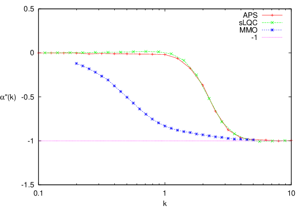
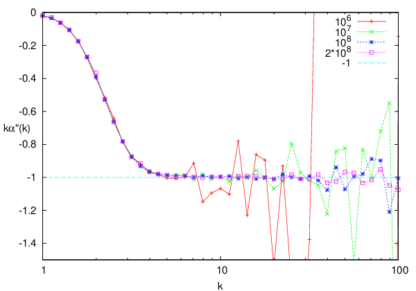
The results are presented in Figs. 1 to 3. As we can see in Fig. 1 the chosen methods allow to calculate quite precisely within the entire investigated domain. Its precise form varies for small depending on the particular prescription, whereas for large the derivative quickly approaches . The rate of approach (59) is confirmed for (see Fig. 2a), however due to the numerical errors the results are no longer reliable for larger . Nonetheless the results converge also there as increases, which is shown in Fig. 2b.
The nd order derivative could be evaluated reliably only for , as it is more sensitive to the numerical errors. The result is presented in Fig. 3a showing the rescaled derivative . From there we observe that it quickly approaches its limiting value deduced from Fig. 1a, never exceeding it [69]. As in the case of the remnant of the numerical results converge as increases, which is presented in Fig. 3b.
References
- [1] C. Rovelli, Quantum Gravity (CUP, Cambridge, 2004).
- [2] A. Ashtekar and J. Lewandowski, Classical Quantum Gravity 21, R53 (2004); T. Thiemann, Introduction to Modern Canonical Quantum General Relativity (CUP, Cambridge, 2007).
- [3] M. Bojowald, Living Rev. Rel. 11, 4 (2008); A. Ashtekar, Gen. Rel. Grav. 41, 707-741 (2009).
- [4] A. Ashtekar, Nuovo Cim. 122B, 135-155 (2007).
- [5] A. Ashtekar, T. Pawłowski, and P. Singh, Phys. Rev. Lett. 96, 141301 (2006).
- [6] A. Ashtekar, T. Pawłowski, and P. Singh, Phys. Rev. D 73, 124038 (2006).
- [7] A. Ashtekar, T. Pawłowski, and P. Singh, Phys. Rev. D 74, 084003 (2006).
- [8] A. Ashtekar, A. Corichi, and P. Singh, Phys. Rev. D 77, 024046 (2008).
- [9] A. Corichi and P. Singh, Phys. Rev. Lett. 100, 161302 (2008).
- [10] E. Bentivegna and T. Pawłowski, Phys. Rev. D 77, 124025 (2008).
- [11] A. Ashtekar and T. Pawłowski, in prep.; W. Kamiński, and T. Pawłowski, Phys. Rev. D 81, 024014 (2010).
- [12] A. Ashtekar, T. Pawłowski, and P. Singh, in prep.
- [13] A. Ashtekar, T. Pawłowski, P. Singh, and K. Vandersloot, Phys. Rev. D 75, 024035 (2007).
- [14] K. Vandersloot, Phys. Rev. D 75, 023523 (2007).
- [15] M. Bojowald, Classical Quantum Gravity 20, 2595 (2003).
- [16] D.W. Chiou, Phys. Rev. D 75, 024029 (2007).
- [17] Ł. Szulc, Phys. Rev. D 78, 064035 (2008).
- [18] M. Martín-Benito, G.A. Mena Marugán, and T. Pawłowski, Phys. Rev. D 78, 064008 (2008).
- [19] M. Martín-Benito, G.A. Mena Marugán, and T. Pawłowski, Phys. Rev. D 80, 084038 (2009).
- [20] A. Ashtekar, and E. Wilson-Ewing, Phys. Rev. D 79, 083535 (2009).
- [21] A. Ashtekar, and E. Wilson-Ewing, Phys. Rev. D 80, 123532 (2009).
- [22] M. Martín-Benito, L. J. Garay, and G.A. Mena Marugán, Phys. Rev. D 78, 083516 (2008); M. Martín-Benito, and G.A. Mena Marugán, Int. J. Mod. Phys. A 24, 2820-2838 (2009).
- [23] A. Perez, arXiv:gr-qc/0409061.
- [24] A. Ashtekar, M. Campiglia, and A. Henderson, Phys. Lett. B 681, 347-352 (2009).
- [25] C. Rovelli, F. Vidotto, Classical Quantum Gravity 25, 225024 (2008).
- [26] A. Ashtekar, W. Kamiński, and J. Lewandowski, Phys. Rev. D 79, 064030 (2009).
- [27] A. Ashtekar, M. Bojowald, and J. Lewandowski, Adv. Theor. Math. Phys. 7, 233 (2003).
- [28] Ł. Szulc, W. Kamiński, and J. Lewandowski, Classical Quantum Gravity 24, 2621-2636 (2007); Ł. Szulc, Classical Quantum Gravity 24, 6191-6200 (2007); W. Kamiński, J. Lewandowski, and Ł. Szulc, Classical Quantum Gravity 25, 055003, (2008).
- [29] W. Kamiński, and J. Lewandowski, Classical Quantum Gravity 25, 035001 (2008).
- [30] W. Kamiński, J. Lewandowski, and T. Pawłowski, Classical Quantum Gravity 26, 245016 (2009).
- [31] W. Kamiński, J. Lewandowski, and T. Pawłowski, Classical Quantum Gravity 26, 035012, (2009).
- [32] P. Singh and K. Vandersloot, Phys. Rev. D 72, 084004 (2005).
- [33] V. Taveras, Phys. Rev. D 78, 064072 (2008).
- [34] See e.g. P. Singh, K. Vandersloot, and G.V. Vereshchagin, Phys. Rev. D 74, 043510 (2006); J. Mielczarek, T. Stachowiak, and M. Szydłowski, Phys. Rev. D 77, 123506 (2008); A. Ashtekar, and E. Wilson-Ewing, Phys. Rev. D 78, 064047 (2008); P. Singh, Classical Quantum Gravity 26, 125005 (2009); G.J. Olmo and P. Singh, JCAP 0901, 030 (2009); M. Artymowski, Z. Lalak, and Ł. Szulc, JCAP 0901, 004 (2009); J. Grain and A. Barrau, Phys. Rev. Lett. 102, 081301 (2009); J. Grain, arXiv:0911.1625; A. Ashtekar and D. Sloan, arXiv:0912.4093.
- [35] A. Corichi and P. Singh, Phys. Rev. D 78, 024034 (2008).
- [36] A. Corichi, and P. Singh, Phys. Rev. D 80, 044024 (2009).
- [37] A. Ashtekar, and M. Bojowald, Classical Quantum Gravity 22, 3349-3362 (2005); 23, 391-411 (2006).
- [38] R. Gambini, J. Pullin, Phys. Rev. Lett. 101, 161301 (2008).
- [39] M. Bojowald, and R. Świderski, Classical Quantum Gravity 21 4881-4900 (2004); 23 2129-2154 (2006).
- [40] M. Campiglia, R. Gambini, and J. Pullin, Classical Quantum Gravity 24, 3649-3672 (2007); R. Gambini, and J. Pullin, Adv. Sci. Lett. 2, 255-260 (2009); R. Gambini, J. Pullin, and S. Rastgoo, Classical Quantum Gravity 26, 215011 (2009).
- [41] C.J. Fewster, and H. Sahlmann, Classical Quantum Gravity 25, 225015 (2008).
- [42] J. Yang, Y. Ding, and Y. Ma, arXiv:0902.1913; Phys. Lett. B 682, 1-7 (2009).
- [43] D.W. Chiou, and L.F. Li, Phys. Rev. D 80, 043512 (2009).
- [44] M.V. Battisti, Phys. Rev. D 79, 083506 (2009).
- [45] G. De Risi, R. Maartens, and P. Singh, Phys. Rev. D 76, 103531 (2007); T. Cailleteau, P. Singh, and K. Vandersloot, Phys. Rev. D 80, 044024 (2009).
- [46] M. Bojowald, Phys. Rev. D 75, 123512 (2007).
- [47] A. Corichi, and P. Singh, Phys. Rev. Lett. 101, 209002 (2008).
- [48] M. Bojowald, Phys. Rev. Lett. 100, 221301 (2008).
- [49] M. Domagała, and J. Lewandowski, Classical Quantum Gravity 21, 5233-5244 (2004); K.A. Meissner, Classical Quantum Gravity 21, 5245-5252 (2004).
- [50] T. Thiemann, Phys. Lett. B 380, 257-264 (1998); Classical Quantum Gravity 15, 839–873 (1998); 15, 1281–1314 (1998).
- [51] M. Martín-Benito, G.A. Mena Marugán, and J. Olmedo, Phys. Rev. D 80, 104015 (2009).
- [52] In comparizon to [7] here we use slightly different representation obtained from the one of APS via unitary mapping .
- [53] D. Marolf, arXiv:gr-qc/9508015; Classical Quantum Gravity 12, 1199 (1995); 12, 1441 (1995); 12, 2469, (1995).
- [54] A. Ashtekar, J. Lewandowski, D. Marolf, J. Mourão, and T. Thiemann, J. Math. Phys. 36, 6456 (1995).
- [55] M. Bojowald, H.H. Hernandez, and H. Morales, Classical Quantum Gravity 23, 3491-3516 (2006).
- [56] W. Kamiński, J. Lewandowski, and T. Pawłowski, unpublished.
- [57] For the simplicity we drop the index , remembering that here we consider just the sector .
- [58] C. Rovelli, Classical Quantum Gravity 8, 297 (1991); B. Dittrich, Gen. Rel. Grav. 39, 1891 (2007); Classical Quantum Gravity 23, 6155 (2006); T. Thiemann, Classical Quantum Gravity 23, 1163 (2006).
- [59] Here the symbols and are defined via requirements that and .
- [60] B. Simon, Adv. in Math. 137, 82-203 (1998).
- [61] The successive derivatives starting from are integrable at .
- [62] M. Bojowald, H. Hernandez, and A. Skirzewski, Phys. Rev. D 76, 063511 (2007).
- [63] G.A. Mena Marugán, private communication.
- [64] W. Kamiński, and T. Pawłowski, in prep..
- [65] M. Reed, and B. Simon, Methods of Modern Mathematical Physics Vol. II (New York: Academic Press, 1978).
- [66] One has to remember that in both APS and sLQC prescriptions the symmetric eigenfunctions considered here have support on both and . Therefore in those cases we have in fact integrals over as well as , whereas in MMO prescription we have just one orientation and one integral. On the other hand, when dealing with symmetric LQC states we should also symmetrize the WDW ones and the orthonormality condition should apply to the symmetrized WDW basis. In consequence, while the derivation is formally formulated just for one orientation (MMO prescription) the final expression (100) remains valid also in the cases of symmetric bases (APS and sLQC prescription).
- [67] E.W. Weisstein, ”Fourier Transform–Heaviside Step Function.” From MathWorld–A Wolfram Web Resource, http://mathworld.wolfram.com/ FourierTransformHeavisideStepFunction.html.
- [68] To be more precise, one should use here the regularization which removes the upper boundary term in the integration if it grows slower than any exponential function.
- [69] The points, for which , observed in Fig. 3a are the result of the numerical errors, see Fig. 3b.