Capacitor Discharge and Vacuum Resistance in Massless
Abstract
A charged parallel plate capacitor will create particle-antiparticle pairs by the Schwinger process and discharge over time. We consider the full quantum discharge process in 1+1 dimensions including backreaction, when the electric field interacts with massless charged fermions. We recover oscillatory features in the electric field observed in a semiclassical analysis and find that the amplitude of the oscillations falls off as and that stronger coupling implies slower decay. Remarkably, Ohm’s law applies to the vacuum and we evaluate the quantum electrical conductivity of the vacuum to be , where is the fermionic charge. Similarities and differences with black hole evaporation are mentioned.
I Introduction
Following Schwinger’s 1951 paper [1], it is well-known that quantum effects cause electric fields to produce electron-positron pairs. The effect can be interpreted as the tunneling of virtual electron-positron pairs into real particles. One imagines a virtual pair produced in the vacuum which is then torn apart by the background electric field, say within a capacitor, with the positron accelerated in the direction of the electric field, and the electron in the opposite direction. A similar effect has been proposed in de Sitter space where the rapid expansion of spacetime “pulls” particles out of the vacuum. Hawking radiation from black holes has also been interpreted as a Schwinger process, though the universally attractive nature of gravity suggests that there are differences. For example, in the electromagnetic case, it is clear that once the charges are created, the positive charge accelerates away from the positively charged capacitor plate due to electromagnetic repulsion. In the black hole case, however, there is radiation even though the black hole attracts all outgoing particles.
The energy for pair creation in an electric field must eventually come from the energy in the electric field itself. Hence the electric field has to decay due to the Schwinger process, just as Hawking radiation is assumed to cause black holes to evaporate. The problem of electric field decay clearly involves calculation of the backreaction of the Schwinger process and this is a hard problem. There have been several attempts to analyze the decay of the electric field by semiclassical methods, replacing quantum operators by their expectation values [2]. The results are interesting. For example, a uniform electric field will not discharge monotonically but will undergo oscillations. If the conclusion can be directly transported to the black hole case, it would imply oscillations of the black hole mass and not monotonic evaporation. A key difference though is that electric charges can be positive or negative, whereas the particles in Hawking radiation can only have positive mass. (See also the recent work [3], where backreaction in the context of scalar QED in 3+1 dimensions was taken into account by solving the equations of motion derived from the one loop Euler-Heisenberg effective action.)
In this paper we re-visit the problem of capacitor discharge due to the Schwinger process, without restricting ourselves to the semiclassical approximation. We can solve the full quantum problem but the price we pay is that we are then only able to treat massless fermions and the exponential suppression of the classic Schwinger process is absent.
We treat the case of massless QED in 1+1 dimensions
| (1) |
The fermions interact with the gauge field by the standard minimal coupling, and an electric field leads to fermion pair production. The advantage of 1+1D QED is that it can be bosonized to yield [7, 8, 9],
| (2) |
where, is the Levi-Civita tensor in 1+1D with and11 1 Note added: Previous versions of this paper contained a spurious factor of in the following formula, i.e., . (We thank Jaume Garriga and Emil Mottola for bringing this to our attention.) We have, accordingly, dropped this factor of in the electrical conductivity of eq. (45), and everywhere in the text referring to it.
| (3) |
where, without any loss of generality, we can assume . The correspondence between the fermionic and bosonic models is given by identifying the currents at the quantum operator level [10]
| (4) |
The bosonized model is particularly easy to solve because it is quadratic in fields and hence there are no interactions. It is sufficient to solve it classically. This simplification only occurs if the fermions are massless in the original model. If we had included a mass for the fermions, we would have obtained a sine-Gordon potential for the scalar field, which is an interacting scalar field theory, and a quantum treatment of the bosonized model would become necessary.
To analyze the discharge of a capacitor, we would like to set up an initial electric field that is localized within a finite region of space and then examine its evolution due to the spontaneous production of fermion pairs. This leads to a physical difficulty because the capacitor plates are necessarily external to the system. This physical difficulty arises even in classical electromagnetism, where Maxwell’s equations are solved but the boundary conditions are provided externally. The difficulty can be avoided in gravitational systems, for example, during gravitational collapse, because the system naturally tends to evolve toward a black hole. On the other hand, if the gravitational problem is set up to include an eternal black hole as an “external” agent, a similar issue arises. There is no analog of gravitational collapse in the electromagnetic situation since similar electric charges repel. If we were to set up a configuration of field corresponding to separated localized positive and negative charges, the charge distributions would simply spread out due to mutual repulsion and then annihilate. Hence an external capacitor plate is necessary to set up the problem.
Here we will set up the capacitor problem in two ways. In the first scheme, we fix the boundary condition that there is a charge at and another charge at . These external charges are taken to be fixed and are non-dynamical. The Schwinger process then creates pairs and dissipates the electric field within the capacitor but cannot “evaporate” the charge on the plates. In this case, we find that the capacitor charges are screened due to the Schwinger process and the electric field decays exponentially with distance from a capacitor plate. Our second strategy to set up the capacitor plates is to introduce an external potential (two “bags”) into which we can insert the charges and as configurations of the field itself. These charges are now dynamical because the field is dynamical. The Schwinger process causes evaporation of the charge from the bags. In both physical realizations, the approach to the asymptotic state is not monotonic but oscillatory. In the first case, the final static state still contains the charges but the charges are screened by opposite charges. In the second case, the final state is not static. Instead it contains bound states of positive and negative charge densities that oscillate without dissipation within the bags.
In the following two sections we describe the discharge of a capacitor in the two physical setups, first with “external charges” and second with “external potential”. We can solve the first setup analytically, allowing us to obtain explicit expressions for the late time behavior of the current, electric field, and energy decay law. The solution of the second setup has only been obtained numerically. The results of both methods are summarized in Sec. IV and show that the capacitor discharge is oscillatory, the root-mean-square current is proportional to the root-mean-square electric field (Ohm’s law), and that the electrical conductivity of the vacuum is equal to .
II Setup I: External Charges
In this section we treat the capacitor as made up of two external charges placed at respectively (see Fig. 1). The electric field due to these charges satisfies Maxwell’s equations and is a non-zero constant in the region between the plates. The value of the electric field in the region is . For , the electric field vanishes. This electric field configuration, together with and , corresponding to no particles, are the initial conditions whose evolution we will consider.
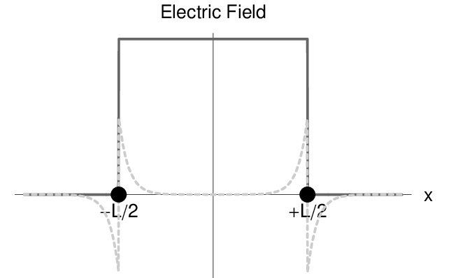
The equations of motion follow from (2). Including the external charges on the capacitor plates, we get
| (5) | |||||
| (6) |
with
| (7) | |||||
| (8) |
and .
Maxwell’s equations (6) can be integrated immediately to get
| (9) |
where
| (10) |
Note that we have set the constant of integration to zero so that the electric field at spatial infinity vanishes.
The charge within some interval is given by Gauss’ law
| (11) | |||||
Inserting (9) into the scalar field equation, (5), gives
| (12) | |||||
where the effective mass of the scalar field is given by the coupling constant,
| (13) |
Hence our problem reduces to solving the Klein-Gordon equation for a scalar field of mass , sourced by the “electric field”, , within the capacitor. The initial condition at is given by the requirement that no fermions be present, or in terms of the bosonic variables,
| (14) |
Before we evolve the equations, however, it is interesting to find static solutions into which the system can evolve asymptotically.
II.1 Static Solution
In the asymptotic future, , we expect the solution to be simply the static solution to (12). Since the Klein-Gordon equation (12) is linear, we may first solve it with i.e. due to a single point charge at the origin. The static solution to the present problem would then follow using appropriate linear superposition. For now,
| (15) |
Using the integral representation of the step-function and that of the retarded Green function, ,
| (16) |
| (17) |
provides us with the integral representation
| (18) | |||||
II.2 Dynamical Solution
The solution to (12) we are seeking must satisfy the initial conditions in (14). To obtain this dynamical solution, we add a homogeneous solution, , obeying , to the static solution such that the initial conditions are satisfied. Again, it helps to first solve the problem with a single charge. Then we have to solve (15) with the initial conditions corresponding to (14). From the conditions in (14), we observe that the integral representation of the solution is
| (23) | |||||
The solution to (12) with the same initial conditions is thus
| (24) | |||||
From this, we can extract the flux of energy passing through a given spatial point and integrate over all time to get the total energy radiated. It is
| (25) | |||||
We first use
| (26) |
followed by
| (27) |
for , to obtain for ,
| (28) | |||||
and, for ,
| (29) |
By considering the limit , we obtain the total energy that is radiated
| (30) |
We can check that the expressions for are consistent with energy-momentum conservation, , if the final field configuration is the static . A direct calculation verifies
| (31) |
with
| (32) |
where the “mass term” in arises from the electric field energy density , since .
One may also use formula 3.876.1 in Gradshteyn and Ryzhik [5]
and apply it to the integral representation (24), to obtain the rate of charge creation, :
| (36) | |||||
where . The first term can be attributed to the charge at whereas the second to the charge at . Charge creation at any location goes to zero at late times because the Bessel functions tend to and hence . This is consistent with the expectation that the asymptotic field configuration is in (II.1).
The electric current at any spacetime location is
| (37) |
where we have introduced and also used . We use a trick to evaluate this integral. Let us first differentiate with respect to . Then after applying appropriate trigonometric identities and Eq. (II.2), this gives
| (38) | |||||
where we have defined . Noting that the current vanishes when the plate separation vanishes (), we get
| (39) | |||||
At late times, , we can Taylor expand the Bessel functions at and then perform the integration over to get
where we have used the asymptotic form of the Bessel function [5] in the second line. The first term is a good approximation for .
The expression in Eq. () shows that the current within the capacitor (say at ) oscillates at the “microscopic” frequency given by . If we average out these fast oscillations, the cosine gets replaced by and we find that the root-mean-squared current decays as :
| (41) |
The electric field within the capacitor decays to a static value that can be obtained from the static solution Eq. (II.1) inserted into (9). The time-dependent electric field within the capacitor at late times can be obtained from the expression for the current in Eq. () together with the asymptotic static solution
| (42) |
To check this expression simply differentiate with respect to time and keep the leading order term in . This agrees with . Note that the static part of the electric field plays no role. In fact, well away from the capacitor plates, the static electric field dies off exponentially fast and can be ignored. So we will define the decaying part of the electric field as and refer to this as the electric field.
The expression for the electric field shows that it is out of phase with the current but the amplitude has the same decay as the current. The rms value of the electric field is
| (43) |
This leads to Ohm’s law
| (44) |
where is the electrical conductivity of the vacuum
| (45) |
This result is independent of and .
Let us now consider the energy in the capacitor. At late times, the fields approach the static solution whose energy can be computed using (II.1)
| (46) |
This shows that the final energy is smaller if the coupling is stronger. Or stronger coupling implies more complete radiation of the capacitor energy.
We can identify a typical time scale for energy loss from the capacitor by considering the ratio of the decaying part of the energy in the electric field within the capacitor at time to the initial energy (). The ratio is
| (47) |
where
| (48) |
Hence larger couplings imply longer decay times i.e. slower decay. The capacitor is more effectively discharged when the coupling constant is large but it takes a longer time for the discharge to happen. In the zero coupling limit, the rate of pair production is rapid, but the original electric field remains relatively undissipated.
III Setup II: External Plates
In the second setup we do not wish to introduce external charges. Instead the capacitor is charged with the same fermionic field, , or its bosonized version, . However we still need to have some capacitor “plates” that we can charge. These plates have to be external to the system. To implement this scheme, we add a double well potential to the action in (2)
| (49) |
where the form of is chosen so that we can find a non-dissipative solution for the scalar field in a single well. A sketch of the setup is shown in Fig. 2.22 2 See [4] for a setup in a similar spirit, but in the context of QCD2.

It is convenient to choose
| (50) |
where is some mass scale that sets the depth and width of the well. With this choice the solution to the single well problem
| (51) |
is given by the kink
| (52) |
where we have chosen the initial condition . The solution describes a positive charge in the well at , which then oscillates – due to pair creation in the electric field – but does not dissipate. The charge in the well at any given time can be found from Eq. (6) to be .
Now consider a capacitor with two plates, one at and the other at . Since we do not have any external charges, we take the constant background electric field, in Eq. (9), to be zero. This means we are now solving
| (53) |
with the following choice of initial conditions
| (54) |
In what follows, we shall set and so all quantities will be in units of .
III.1 Asymptotic State
Before solving for the time evolution, we consider the asymptotic state, which will be a stationary solution of Eq. (53). That is, we think of the double well equation (53) as a Schrodinger equation
| (55) |
with Hamiltonian
| (56) |
The corresponding Hamiltonian for a single potential well centered at is
| (57) |
This has exactly one bound state
| (58) |
with eigenvalue [6]. (Recall that we are working in units with .) So for the double well potential, at least when the two wells are well separated, there must be exactly two bound states, which can be approximated as
| (59) |
The energies of these two bound states are nearly identical, , , split by exponentially small corrections due to tunneling between the double wells. These bound states are the stationary states that the system can evolve into.
We also observe that there is an apparent instability in the current model when , since then and the bound state solution can grow exponentially. To understand this instability, we examine the double well action in (49). If the potential is deep enough, there will be a region where is sufficiently negative, that it becomes favorable for to grow without bound in this region. In terms of the fermionic model, the well is so deep that it is favorable to pull fermion pairs out of the vacuum and put them at the bottom of the potential.
The evolution of the initial data, , in this setup can be evolved formally by writing
| (60) |
where the summation is over both bound and continuum states of . We can check that the initial conditions are satisfied by setting in the factor and in its time derivative. We expect that, as time progresses, the continuum states will disperse to infinity, leaving behind only the initial overlap with the bound state. While formally correct, the expansion in Eq. (60) is only useful if we know the full eigenspectrum of the double well potential. In the absence of the eigenspectrum, it is easier to numerically evolve the equation of motion.
III.2 Time Evolution
We have evolved Eq. (53) using the explicit Crank-Nicholson algorithm with two iterations with first-order absorbing boundary conditions. The runs were done on very large lattices so that boundary effects are minimal.


In Fig. 3 we plot the current envelopes at versus time for several different parameters, disregarding the rapid oscillations between the envelopes. Similarly, in Fig. 4 we show the behavior of the electric field at . On the log-log plot in Fig. 5, it is clear that the envelopes decay as a power law. A fit gives
| (61) |
where is a factor which could depend on the dimensionless product , where is the width of the wells (see Eq. (50)). The electrical conductivity is therefore again given by Eq. (45), as for setup 1.


IV Conclusions and Discussion
We have studied the quantum discharge of a capacitor in massless QED in 1+1 dimensions by bosonizing the model. The bosonized model is non-interacting and can be solved classically. The solution includes all backreaction effects. We now summarize the key results.
The final state depends on the setup used to describe the capacitor plates. We have chosen two different ways to describe the capacitor plates. In both cases, the final state is non-trivial. In setup I, the plates keep their original charge but the charges are screened due to the Schwinger process. In setup II, there are no external charges, but there are external potentials that play the role of capacitor plates. Then the final state consists of fermion-antifermion pairs that are bound to the plates.
The energy in the final state depends on the coupling constant, , and equivalently the mass of the scalar field, . The final state energy decreases with increasing , while the time for the capacitor to discharge increases with increasing , as seen in Eq. (48). So stronger coupling leads to more complete discharge but the discharge process itself is slower. We suggest that the longer discharge time for larger coupling constant is due to the tighter binding of fermion-antifermion pairs that need to be split apart by the electric field.
The discharge process is highly oscillatory, as also seen in the semiclassical analysis [2] and the amplitude of oscillations falls off rather slowly, as . This suggests that the massless QED system is under damped
Our results show that the root-mean-square current in the capacitor is directly proportional to the root-mean-square electric field, indicating that Ohm’s law holds on a macroscopic scale. Thus it makes sense to define the electrical conductivity for the massless QED vacuum to be and our results indicate the simple relation which can also be written in terms of the fermionic charge as .
A correspondence is often made between Schwinger pair creation and Hawking radiation, though we have indicated differences between the two processes that prompt us to use caution in drawing a correspondence. If the oscillatory features of the discharge process carry over to black hole evaporation, we may expect black hole mass oscillations during evaporation. Though, in contrast to the capacitor, the black hole system is unstable in that smaller mass black holes are hotter and evaporate faster, while weaker electric fields in the capacitor do not discharge faster. So it would appear that a fluctuation that excessively decreases the mass of the black hole, would make it evaporate yet faster in what may be a runaway process.
The issues of black hole formation and the final state of black hole evaporation cannot be resolved by this correspondence since the capacitor plates have to be introduced externally, whereas there are no such externally set conditions in the case of gravitational collapse. Yet it would be extremely interesting if the electromagnetic Ohm’s law has a gravitational analog that relates energy flow (current) from a black hole, or during gravitational collapse, to the “gravitational electric” field (see Sec. 4.4 of [11]). Perhaps the instability of the black hole can be summarized in a negative “gravitational conductivity”.
A potential application of our findings is to superconducting cosmic strings, where massless QED in 1+1 dimensions is expected to apply for fermion zero modes on the string [12]. Our analysis shows that if superconducting strings really behave as 1+1 dimensional systems, they will carry oscillatory currents because of the backreaction of the induced currents on the external electric fields. (Oscillatory currents were also discussed in [13], though these occurred due to the periodic dynamics of the strings.)
While our analysis has enabled us to fully treat backreaction of the Schwinger process, our results cannot be transported to 3+1 QED for two reasons. First, the electron has a non-zero mass. For electric fields smaller than the electron mass squared, the Schwinger process is exponentially suppressed and the vacuum is essentially an insulator. In situations where the electric field is larger than the electron mass squared, the exponential suppression is absent and the dynamics may be closer to what we have found. The second reason is that the larger number of dimensions can change the picture dramatically. In 1+1 dimensions, the inter-charge potential is linear and electric charge is confined. In 3+1 dimensions, electric charges interact by the Coulomb potential and are not confined. This suggests that our system may be closer to the case of chromo-electric fields in 3+1 dimensions with massless quarks. While this has some features that resemble the model we have considered, there are essential differences due to the non-Abelian nature of the interactions.
Acknowledgements.
We thank Edward Witten for suggesting the massless Schwinger model for the backreaction problem, Ioannis M. Besieris for sharing his notes on the solution to the massive Klein-Gordon equation, and Ratin Akhoury, Daniel Green, Zohar Komargodski, Juan Maldacena, Dmitry I. Podolsky, David Shih and Yuji Tachikawa for helpful comments and discussions. We thank Peter J. Kernan and Pascal M. Vaudrevange for invaluable computing help. This work was supported by the U.S. Department of Energy at Case Western Reserve University. TV was also supported by grant number DE-FG02-90ER40542 at the Institute for Advanced Study.References
- [1] J. S. Schwinger, Phys. Rev. 82, 664 (1951).
- [2] Y. Kluger, J. M. Eisenberg, B. Svetitsky, F. Cooper and E. Mottola, Phys. Rev. D 45, 4659 (1992). Y. Kluger, J. M. Eisenberg, B. Svetitsky, F. Cooper and E. Mottola, Phys. Rev. Lett. 67, 2427 (1991). F. Cooper and E. Mottola, Phys. Rev. D 40, 456 (1989).
- [3] E. T. Akhmedov and P. Burda, arXiv:0912.3435 [hep-th].
- [4] D. Bazeia, F. A. Brito, W. Freire and R. F. Ribeiro, Int. J. Mod. Phys. A 18, 5627 (2003) [arXiv:hep-th/0210289].
- [5] I.S. Gradshteyn and I.M. Ryzhik Table Of Integrals, Series and Products, fourth edition, Academic Press, New York (1980).
- [6] P. M. Morse and H. Feshbach, Methods of Theoretical Physics, Part II, McGraw Hill (1953), §12.3
- [7] S. R. Coleman, R. Jackiw and L. Susskind, Annals Phys. 93, 267 (1975); S. R. Coleman, Annals Phys. 101, 239 (1976).
- [8] K. Fujikawa, arXiv:0902.2066 [hep-th].
- [9] C. M. Naon, Phys. Rev. D 31, 2035 (1985).
- [10] J. von Delft and H. Schoeller, Annalen Phys. 7, 225 (1998) [arXiv:cond-mat/9805275].
- [11] “General Relativity”, R.M. Wald, University of Chicago Press, Chicago (1984).
- [12] E. Witten, Nucl. Phys. B 249, 557 (1985).
- [13] M. Aryal, A. Vilenkin and T. Vachaspati, Phys. Lett. B 194, 25 (1987).