August 24, 2026
LA-UR-10-0063
arXiv:1001.2514
Solving the Radial Dirac Equations: A Numerical Odyssey
Abstract
We discuss, in a pedagogical way, how to solve for relativistic wave functions from the radial Dirac equations. After an brief introduction, in Section II we solve the equations for a linear Lorentz scalar potential, , that provides for confinement of a quark. The case of massless and quarks is treated first, as these are necessarily quite relativistic. We use an iterative procedure to find the eigenenergies and the upper and lower component wave functions for the ground state and then, later, some excited states. Solutions for the massive quarks (, , and ) are also presented. In Section III we solve for the case of a Coulomb potential, which is a time-like component of a Lorentz vector potential, . We re-derive, numerically, the (analytically well-known) relativistic hydrogen atom eigenenergies and wave functions, and later extend that to the cases of heavier one-electron atoms and muonic atoms. Finally, Section IV finds solutions for a combination of the and potentials. We treat two cases. The first is one in which is the linear potential used in Sec. II and is Coulombic, as in Sec. III. The other is when both and are linearly confining, and we establish when these potentials give a vanishing spin-orbit interaction (as has been shown to be the case in quark models of the hadronic spectrum).
pacs
02.30.Hq, 02.60.Lj, 12.39.Ki, 31.15.B-I Introduction
Dirac formulated relativistic quantum mechanics in the late 1920’s.[1] Since field theory had not yet been developed, the relativistic aspect led to a number of confusions related to currents since only total charge is conserved. With the recognition of the appearance of antiparticles, and the development of field theory, analogous to the transition from the Canonical to the Grand Canonical ensemble in statistical mechanics, these issues were resolved. Nonetheless, the solution of the equation itself, ignoring these deeper aspects, has proven valuable even in more modern contexts.
For example, the MIT bag model of quark confinement,[2] and the theories that evolved from it (chiral bag, cloudy bag, etc.)[3] depend on solving the Dirac equation as a wave function for a particle in an effective potential. Through boundary conditions and other approximations, the Dirac equation has even been employed in this way in the study of nuclear structure.[5, 4]
In particle physics, the quark model has been employed, with great success, to describe baryon and meson states and their structure. Usually this is done in a non-relativistic model, [6] where the potentials follow the patterns expected by a Foldy-Wouthuysen reduction[7] of a simpler, theoretically motivated potential in the Dirac equation. In our case, however, we wanted to see how these structures and solutions appear without the non-relativistic reduction approximations, by solving the Dirac equation itself for the simpler potential with fewer adjustable parameters.
Going back somewhat in time, very soon after Dirac’s initial formulation, Darwin [8] found an analytic solution (!) for the radial wave functions for hydrogen-like atoms in terms of confluent hypergeometric functions. Since then, solutions of the Dirac equation have been important in atomic physics, even to recent times.[9, 10] For example, more complicated central potentials than , the fourth component of a Lorentz four-vector, usually require finding a numerical solution. Another example is a muonic atom, in which a muon is in an s-state about a heavy nucleus having a realistic charge distribution.[11]
Finding such numerical solutions involves solving coupled ordinary differential equations for the upper and lower components of the Dirac wave function, [12, 10]
| (1) |
where and the are the spin-orbital angular momentum wave functions,
| (2) |
where is a Clebsch-Gordan coefficient and is a Pauli spinor.
We consider here the case of bound-state wave functions for a central potential with energy eigenvalue . For example, for hydrogen-like atoms the potential is . With appropriate boundary conditions, the radial wave functions and , which can be taken as real functions, are solutions of the following coupled first-order ordinary differential equations (ODEs), [12, 9]
| (3) | |||||
| (4) |
Here the integer is determined by the angular momentum quantum numbers according to
| (5) |
The reason for the subscript on the potential in those equations is to indicate that it is the fourth component of a Lorentz four-vector, such as the Coulomb potential. However, our motivation is not so much in atomic physics applications as it is for treating mesons as states in a relativistic quark model. The non-relativistic quark model often assumes the confining potential for quarks to be the so-called “Cornell potential,” [6]
| (6) |
where , with being the (running) quark-gluon coupling constant, and (or ) is the string tension. It is the linear term in that confines the quarks, corresponding to the effective potential in the relativistic Bag Model.[2]
For a relativistic quark model, the two pieces of that non-relativistic potential have different Lorentz transformation properties. The color Coulomb potential, , is the fourth component of a Lorentz vector, while the confining linear potential transforms as a Lorentz scalar, which we will write as . Thus, in solving the relativistic radial Dirac equations, the two terms in the non-relativistic potential of Eq. (6) enter the coupled ODE’s differently. The equations to be solved are
| (7) | |||||
| (8) |
Note that in these equations the sign for is opposite to that of the energy eigenvalue , the fourth component of the momentum four-vector, while that for matches that for the fermion mass , also a Lorentz scalar.
So, we were motivated to study solutions of Eqs. (7) and (8). After submitting an earlier version of this paper to the archives, we learned of related studies of these equations by Paris[14] and by Soares de Castro and Franklin[15], who discussed analytic solutions. We, however, have adopted a numerical approach and, in this paper, we discuss how to go about solving these coupled ODE’s numerically. The presentation follows our numerical journey more or less historically. Our hope in writing this paper is that, by reading it, students might avoid some of the pitfalls we encountered and then overcame.
It turns out that solving for a linear scalar potential [16, 4] is quite a bit easier (numerically) than the relativistic hydrogen atom, so we treat that first in Sec. II. We then turn, in Sec. III, to the problems we had with in solving the radial equations for a Coulomb-like potential for hydrogen-like atoms and how we dealt with them. This is followed, in Sec. IV, by a discussion of the mixed problem having both a scalar and a vector potential, as in Eqs. (7) and (8).
II Linear Scalar Potential
For the case of massless quarks (an approximation we have made [13] for the and quarks), we want to solve the equations for a confining linear scalar potential, [16, 4]
| (9) |
where (with ), has dimensions of fm-1. The negative offset, , effectively gives these quarks a constituent mass.[4] It also provides a rough representation of the effect of how the short-distance color Coulomb interaction between quarks leads to quark confinement, albeit without the correct Lorentz representation properties.
The case of massless quarks exhibits the role of relativity in a maximal way, meaning that the lower component is comparable in size to the upper component . We will, later, choose an appropriate mass for the massive quark flavors, , , and , and solve for those wave functions. In these cases, as the quark mass increases, becomes smaller relative to , reflecting the transition to a non-relativistic limit where vanishes. Also, as will be seen, with increasing mass , the heavier quark radial wave functions are progressively narrower than in the massless case. Thus we will, in Sec. IV, also include the effects of a color Coulomb-like vector potential coming from one-gluon exchange. This should prevent a too-rapid fall-off of the quark-quark interaction energies as the quark masses increase [17], but that is a matter for a separate paper.
It simplifies the equations if we convert the ODEs to dimensionless form, dividing through by and defining a dimensionless distance :
| (10) | |||||
| (11) |
where , , and are now also dimensionless.
Numerical integrations of these equations can be done by one or another of the Runge-Kutta methods.[18] To integrate these two first-order ODEs one needs to specify two boundary conditions (BCs) at the place where one begins the integration. However, as the radial wave functions eventually need to satisfy a normalization condition,
| (12) |
this will determine one of the BCs, for example, the scale of the wave functions at asymptotically large distances.
II.1 Shooting Outwards
In our first attempt to solve these equations we thought to integrate them outward from the origin with the hope of adjusting the energy eigenvalue to assure that both and fall off to zero asymptotically. The first problem in doing this is the singularity in the equations at . This singularity, however, is easily avoided by starting instead at a small value of away from the origin.
For starting values (BCs) we can take advantage of the expected power-law behaviors of and near the origin for their known orbital angular momenta and . For example, if , for which and the lower component’s , one can choose
| (13) |
as motivated by the non-relativistic limit, where at small . Substituting this into the second ODE allows us to determine :
| (14) |
The parameter at this point is arbitrary for now and will be fixed later by the normalization condition, Eq. (12).
The problem with simply shooting outwards is what to choose for the energy . The ODE solver for almost all initial guesses for will have the well-known problem that the calculated and very soon blow up exponentially, either positively or negatively. It might be possible to iteratively refine the guess for to eventually find decaying solution, but we soon decided to try a different method.
II.2 Shooting Inwards
A better way of assuring decaying solutions is to start from an asymptotic distance, where that behavior is built-in, and integrate the ODEs inward toward the origin. At large distances the ODEs simplify, for this potential, to
| (15) |
which have solutions at large ,
| (16) |
Note that this asymptotic behavior is the same as that of the non-relativistic simple harmonic oscillator wave functions.[16] These forms will be used as starting values (BCs) for the inward integration of the full ODEs from . Again, can be taken as arbitrary for now, to be later fixed by the normalization condition, but we need to make an initial guess for the energy eigenvalue . The integration will go from back to , again to avoid the singularity at .
The problem with this shooting inwards method is much the same as that for shooting outwards. Unless one somehow is able to guess the exact value of , the solutions will blow up exponentially as one nears the origin, and usually well before that.
II.3 Shooting In and Out and Matching
Thus, after experiencing these well-known problems with ODEs with eigenvalues, we concluded that we had to combine the two methods, invoking a well-known numerical method, “shoot and match.” In this case we shoot both outwards from to a point in the middle, , and inwards from back to . The two values for and will generally differ for a given choice of and another parameter, which we choose to be . That is likewise the case for and . What we therefore need is to find a way to iteratively vary and to reduce the two gaps, and , to zero. [The asymptotic parameter is chosen to be fixed, i.e., not to be varied, but of a size that makes the initial determination of the gaps at reasonably small; it will in the end be determined by the normalization condition, Eq. (12).]
We need to define the gaps , etc., at the match point. Initially, we simply chose them in terms of their actual differences,
| (17) |
and likewise for , , and . Indeed, this often works for the problem we originally set out to do, namely, to calculate wave functions for the (nearly) massless and quarks. However, as the quark mass increases, the system becomes more and more non-relativistic. This means that the lower component wave function, , becomes relatively small compared with . Thus a better definition for the gaps would be to make them relative to their average value, e.g.,
| (18) |
and likewise for .
II.4 Zeroing the Gaps
The two gaps can be driven to zero by using a generalized Newton-Raphson method. First, recall how one derives the Newton-Raphson method for finding the zero of a function . Make an initial guess for the solution, call it . To find a better guess, , expand in a Taylor’s expansion,
| (19) |
As we want the left-hand side to vanish, the next (and better) guess for the root is
| (20) |
This procedure can be repeated until is small enough to be considered zero.
The generalization of Eqs. (19) and (20) for our problem is to solve a two-by-two linear system for new values of the parameters, and , from these equations:
| (21) |
We will calculate the partial derivatives needed above numerically. The procedure to find better values of the two parameters and is to be iterated until the gaps are sufficiently small.
To solve this linear system in Eq. (21), it is convenient to define a matrix
| (22) |
and a column vector containing the gaps and partials obtained using the old parameters and ,
| (23) |
Multiplying by the inverse matrix then provides us with a column vector containing the improved parameters for the next iteration:
| (24) |
It turns out that this iterative procedure works very well, with the gaps in the slopes of and at the match point also going to zero.
At this point we should remark that others might have done this calculation but by zeroing the gaps in the logarithmic derivatives, such as. This has the advantage of removing the scale dependence of the functions and , but our choice of defining the gaps as relative, as in Eq. (18), is essentially equivalent, as it also involves (semi-)local differences divided by the (semi-)local value.
II.5 The Radial Wave Functions and Some Programming Details
We implemented the iterative numerical process discussed above by developing Mathematica notebooks, [19] but any reasonable programming language could be used instead. An example notebook is available from our group’s web site.[20] (We especially invite our Canadian colleagues to convert this to a Maple program!) Here, as we describe the calculation of the ground state radial wave functions for the GMSS potential of Eq. (9), we will comment on a number of the programming issues that we encountered.
The first thing to be done is to set the value of in the equations to be solved. It is an integer and depends upon the angular momentum quantum numbers, Eq. (5). For the , ground state, , , and thus .
As noted earlier, we work in units where [21] so that the dimensions of Eqs. (7) and (8) are fm-1. For the cases discussed here and below, we have fixed the constants in the GMSS potential at (i.e., ), and fm. Making the equations dimensionless, as mentioned after Eq. (11), this linear scalar potential simplifies to , where .
For dimensionless distances we chose , , and . We also define a small increment , which will be used when we calculate the partial derivatives in Eq. (22) numerically and for testing when the gaps to be zeroed are small enough.
The two integrations, inwards and outwards, were done using Mathematica’s NDSolve function, but one could use any standard Runge-Kutta procedure.[18] To proceed, we need the four boundary conditions (BCs) from Eq. (13) and Eq. (16). We have defined a subroutine, shootinandout, to do this. This subroutine is, of course, a function of the parameters and . It saves the results of the integrations as insoln and outsoln, respectively.
In this case, we already had a good idea [4] of what the energy eigenvalue is for the ground state. After some fiddling, we found an initial choice of parameters
| (25) |
for which the resulting outwards and inwards integrations yielded the curves for and shown in Fig. 1. (As mentioned above, the asymptotic normalization is at this point arbitrary, to be fixed later by the normalization condition.)
It is useful at this point to define a function, calcmatchgaps, that uses insoln and outsoln to calculate and print out the values of and at the match point , along with their slopes and their gaps scaled as in Eq. (18). These numbers provide guidance as to how to proceed when developing the Mathematica notebook.
Next, we need the four partial derivatives in the two-by-two matrix of Eq. (22). In pseudocode, the subroutine for calculating is
   subroutine dggapbydE(tildeE,a0)
      delE = delta*tildeE
      outsoln1 = outward integration with parameters (tildeE + delE,a0)
                 from epsilon to xmatch
      g_out1 = g(x) at x_match from outsoln1
      insoln1 = inward integration with parameters (tildeE + delE,a0)
                from xmax to xmatch
      g_in1 = g(x) at x_match from insoln1
      ggap1 = 2.0*(g_out1 - g_in1)/(g_out1 + g_in1)
      dggapdE = (ggap1 - ggap)/delE
      return dggapdE
      end subroutine
Similar subroutines are also implemented for the three other partial derivatives. We also found it useful, once these subroutines were in place, to define another subroutine, gapsandpartials, which calls shootinandout for the present values of the parameters and , followed by calls of calcmatchgaps and the four subroutines for the partial derivatives.
At this point we are ready to solve the two-by-two linear system for improved values of the parameters and . Manipulating arrays is a bit tricky in a programming language such as Fortran or C, but in Mathematica one can simply define the matrix in Eq. (22) as a list of lists and the column vector is a simple list. Mathematica also provides a built-in function to invert the matrix , so the evaluation of the right-hand-side of Eq. (24) is easy. This procedure is encapsulated in a subroutine we called solvelinsys().
Before going on to the program for the iterative loop we need to decide when the gaps are small enough to stop the iteration. Thus we defined a test function which returns a boolean True if any of the four gaps, and as well as their slopes , and , is greater than . Again, in pseudocode,
   subroutine testgaps()
      boolean p1 = Abs[ggap] > delta
      boolean p2 = Abs[fgap] > delta
      boolean p3 = Abs[gpgap] > delta
      boolean p4 = Abs[fpgap] > delta
      boolean q = p1 OR p2 OR p3 OR p4
      return q
      end subroutine
The iteration will stop when q = False.
The coding for running the iteration from an initial choice of parameters and is as follows:
   {newtildeE,newa0} = {start_tildeE, start_a0}
   print starting parameters {newtildeE, newa0, a1}
   iter = 0
   q = True
   do loop
      iter = iter+1
      {oldtildeE,olda0} = {newtildeE,newa0}
      shootinandout(oldtildeE,olda0)
      gapsandpartials(oldtildeE,olda0)
      solvelinsys()   // returns improved values of newtildeE and newa0
      print iter and gaps
      print newtildeE and newa0
      if q
         continue to next iteration, i.e., go to the top of the do loop
      else
         stop and break out of the do loop
      end if
      end do loop
For the starting parameters used above, and , we find that our program closes the gaps in four iterations. The final parameter values are and . That correponds, in more conventional units, to an energy of GeV. Figure 2 shows plots of the final, converged and after normalization. Note the relatively large size of the lower component , showing the importance of relativity in this case of massless quarks.
Figure 3 shows the corresponding plots for and . As one ought expect for a ground state wave function, the upper component has no nodes and the -wave lower component has one (at the origin).
We have plotted the ’s in Fig. 3 this way to compare with GMSS’s Fig. 2. The ’s here are for fitting the non-strange mesons and extend out further than those of GMSS. The reason for that is that GMSS calculated the and quark wave functions to fit the non-strange baryon spectrum, which is why they used a value of . Physically, the effective origin of the confining potential for mesons is not as strongly localized as in the baryon case, where one more quark damps fluctuations additionally.
II.6 Some Excited States
The procedure outlined in the previous sub-section can be applied to calculate the energy eigenvalues and wave functions for excited states. One expects that the first excited state is the state. This state also has , and , so the BCs at are the same as for the case. The upper component wave function should now have a new node, i.e., cross the -axis somewhere between the origin and infinity. Thus, if it is desirable to have start off from the origin going positive, one should choose the asymptotic normalization parameter to be negative.
In view of the asymptotic behavior here being similar to that of a simple harmonic oscillator, we might expect that the energy eigenvalue of this state is roughly twice that of the ground state. Choosing the parameters needed for the initial integrations to be
| (26) |
the iterative loop again converges in four iterations. The final parameters are (i.e., 0.809 GeV) and . Plots of and are displayed in Fig. 4. For the state, has one node and has two.
Why are we counting nodes, anyway? Because a state with more nodes has more energy. Qualitatively, more nodes means more curvature, and that means a bigger contribution from , which in turn means a bigger kinetic energy.
Besides the state, there are also two nearby -wave excited states. The state also has , but now with , , and thus . The BCs near the origin are given by Eqs. (13) and (14), but otherwise the coding is very similar to (basically can be copied from) the and cases. Starting this time with
| (27) |
the gaps close in four iterations, with final parameters (i.e., 0.940 GeV) and . The wave functions and are shown in Fig. 5. In contrast to the case, here both and have two nodes, reflecting a higher energy eigenvalue.
The other -wave state, , is qualitatively different. This is the first case for which , and is now a positive integer. In a sense, this switches the roles of and . The boundary conditions for the outward integration when are different from those of Eq. (13):
| (28) |
Substituting into the first ODE allows us to determine this , so
| (29) |
That is, if , both and start out from the origin with positive slopes.
Starting for this case with initial parameters
| (30) |
the iterative procedure converges on the fifth iteration, with final parameter values (i.e., 1.002 GeV) and . The ’s are plotted in Fig. 6. Here also both component wave functions have two nodes.
We note in passing that the higher spin state of this pair has the lower energy, contrary to the well-known case for the Coulomb potential. This is a common feature for nuclear states (even ground states) and reflects the presence of an effective scalar potential as found in many nuclear potential models.[23]
The energy difference between the and states, 62 MeV, is due to a spin-orbit interaction. However, there is evidence in the meson spectrum that the spin-orbit interaction is suppressed.[24] Page, Goldman, and Ginocchio (PGG) [25] claim this reflects a cancellation between a scalar potential and a vector potential, , having the same linear slope at large distances. We will return to this point in Sec. IV.
II.7 Solutions for Massive Quarks
The cases for the linear scalar potential of Eq. (9) when the quarks are massive are computed straightforwardly using the program described above. For example, using masses appropriate [22] for the mesonic states, where stands for a massless non-strange quark ( and ) and for the massive strange (), charmed (), and bottom () quarks, we find the following eigenenergies:
| (31) | |||||
| (32) | |||||
| (33) | |||||
| (34) |
by requiring a match to the appropriately weighted average of the lowest pseudoscalar and vector states.[26] Note that for the heaviest quarks the states are conventionally bound, , and confinement need not be invoked to understand the stability of the state, in contrast to the situation for the light quarks.
Figure 7 compares the results for the , , , and quarks for the upper components, , and Fig. 8 does the same for the lower components, . Note that as the mass increases, the system becomes more and more non-relativistic, i.e., the lower component wave function gets smaller, relative to the upper component . Also, as gets larger, the wave functions are more and more concentrated near the origin.
III Vector Potential – Hydrogen-like Atoms
In contrast with the case of massless quarks, an electron bound in a Coulomb potential, as in the hydrogen atom, is at the opposite extreme, i.e., is to a very good approximation a completely non-relativistic system. The binding energy of the ground state, Ry = 13.6 eV, is very small compared to the mass of the electron, MeV. (In this section we will use MeV instead of GeV.) The Schrödinger equation for this problem predicts its energy levels basically correctly, missing only the fine-structure splitting, a spin-orbit effect about times smaller than the binding of the levels.[27].
As noted in the Introduction, the analytic solutions of the Dirac equation for the hydrogen atom were found long ago, [8] and these solutions do give the fine-structure splitting as a relativistic effect. Nonetheless, it is an interesting numerical exercise to see if the program for the linear scalar potential outlined above (or something like it) can be applied to the hydrogen atom case, and with enough accuracy. We want to solve Eqs. (3) and (4) with . We will set , as these solutions are somewhat more delicate. Heavier, hydrogen-like atoms with can be done in a similar manner.
Converting to dimensionless equations by dividing through by (instead of as before),
| (35) | |||||
| (36) |
where now and . The energy is better written as , where is the binding energy of the level of interest (which has principal quantum number and orbital angular momentum quantum number ). Note that, because of the smallness of the binding energies, is only slightly less than . Thus is less than (but very close to) 1, which is why we factored out a minus sign from the third term in Eq. (36), relative to that in Eq. (4). We will use the binding energy instead of as one of the two parameters to be determined in the matching of the inwards and outwards integrations.
III.1 Boundary Conditions for Inward Integration
For asymptotically large the ODEs reduce to
| (37) |
The solutions of these asymptotic equations at are
| (38) |
which will be used as the BCs (starting values) for the inwards integration with as another parameter to be determined later by the normalization condition. The coefficient in the exponential decay is small:
| (39) |
The Coulomb wave functions are quite long-ranged, and are all the more so the smaller the binding energy. Equation (38) also shows that, asymptotically, is very much smaller than . The smallness of the lower component is an indication of how non-relativistic the hydrogen atom is.
III.2 Boundary Conditions for Outward Integration
As before, to avoid the singularity at , we integrate outwards from , where takes an appropriately small value. In this case, one might even consider taking as the radius of the nucleus providing the Coulomb potential (but see Sec. III.6 for a better approach). For the boundary conditions for integrating outwards from when , i.e., and , we can again assume
| (40) |
Substituting these in the second ODE, we can solve for , finding
| (41) |
Noticeably different is the lowering of the power behavior of due to the behavior of the potential. Note that, because of the factor of , the magnitude of is much smaller than that of , also here near the origin.
For the case, i.e., and , we let determine the nature of the boundary conditions [as in Eq. (28)], i.e.,
| (42) |
Substituting these in the first ODE, we again solve for and find
| (43) |
Again, for this case, and start off with the same slope, as in Eq. (29). And again, there is a lower power behavior of due to the in the potential, as in Eq. (41).
III.3 The Ground State
The natural unit of length for the hydrogen atom problem is the Bohr radius, Å fm. Thus a natural scale for is in units of the dimensionless Bohr radius, which is in units.
In view of the slow exponential decay in Eq. (38) (i.e., the smallness of ), for our calculations we chose , along with . Fixing (recall, it is arbitrary before normalization) and the starting values of the parameters to be tuned, MeV (less than the expected 13.6 eV) and , we found the matrix of partial derivatives to be
| (44) |
This shows a big sensitivity of the hydrogen atom wave functions to the choice of binding energy. Nonetheless, the iterative process of refining and proceeds nicely to a solution with eV and . The wave functions and are displayed as the solid curves in Figs. 9 and 10. As expected, is much smaller than . Their shapes differ from those shown for the scalar linear potential shown in Fig. 2.
Figures 9 and 10 also display, as dashed curves, the corresponding and radial wave functions. These are, in fact, both purely decaying exponentials proportional to . This is not surprising for the upper component, , since that is the just what the Schrödinger equation predicts for the hydrogen atom ground state. It may not be so obvious, however, that the lower component, , has the same form. That it has no node at the origin (in contrast to Fig. 3) is a consequence of the potential changing the presumed -dependence of near the origin to an -dependence.
III.4 Some Excited States
The excited states of hydrogen are done in a very similar manner to the ground state calculation. The major difference is that, from the Balmer formula [27], we expect the binding energy for these states to be about times the ground state binding energy. Also, based on Eq. (39), we expect the wave functions will extend outward about twice as far, so, for our calculations we chose instead of .
For the state, starting with initial parameters eV (presumably low), , and (fixed) , the program converges in four iterations to give final eV and . The wave functions are plotted in Figs. 11 and 12. As expected on general grounds, unlike the ground state, here and each have one node.
For the state, starting with initial parameters eV (also presumably low), , and (fixed) , the program converged in four iterations to give final eV and . In fact, the and levels are degenerate [27] as a result of an symmetry hiding in the equations. The small difference in the converged ’s we find here is within the numerical precision of our Mathematica program. However, the and wave functions are very different. The wave functions are shown in Figs. 13 and 14. Note that, here also, and each have one node.
For the state, starting this time with initial parameters eV, , and , the program converged in four iterations to give final eV and . The difference we find between the and energy levels, 0.58 meV, is the spin-orbit splitting, an intrinsically relativistic effect. The analytic value of this splitting is 0.453 meV [9, 27] and the difference here is due to the limited machine precision used in our Mathematica program. The wave functions are shown in Figs. 15 and 16. The ’s for the and states are very similar, but the lower component ’s are quite different, reflecting the fact the lower components and the difference are both entirely due to relativity. For the state also, and each have one node.
III.5 Hydrogen-like Atoms with
There are no big surprises here, as Table I shows. From Eq. (39), the exponential fall-off of the wave functions is faster, as , so we adjust the values of and accordingly by dividing the hydrogenic values by . Running the code for the ground state for works well for . As grows larger, the relativistic corrections to the energy become increasingly important.
As approaches , however, the numerical solutions become inaccurate and, eventually, unstable. This can be seen in the rapid increase in the value of the parameter . The value of is where the Klein paradox [28] comes into play, since the analytic result for this state is [12]
| (45) |
and the eigenenergy becomes complex beyond that point. The resolution of this paradox is, as has been well-known for a long time, the creation of electron-positron pairs from the Dirac-Fermi sea when .[29]
III.6 Muonic Atoms
When a negatively-charged muon slows down in matter, sometimes it is captured by the Coulomb potential of an atomic nucleus before it decays. If so, it then quickly cascades down through its hydrogen-like levels to the ground state, emitting x-rays along the way. From there it then either decays or can be be captured by the nucleus, both of which are weak interaction processes. The capture process depends sensitively upon the value of the wave function at the origin.
The numerical coding for muonic atom ground states for values of of interest goes pretty much as for the electronic atom case for such a . The differences come from replacing the mass of the electron (0.511 MeV) with that of the muon (105.66 MeV). This must be done for the “muonic Bohr radius”, = 255.8 fm, and consequently in the choices of and which are now proportional to . Also, the non-relativistic binding energy is now Ry.
Calculating, as above, the ground state for muonic 40Ca (), starting with MeV and = 0.1, the iterations converge to final values of MeV and . However, this initial calculation used a value of (dimensionless), or a cut-off at the origin of 0.000187 fm, rather smaller than the size of the 40Ca nucleus,[30]
| (46) |
The nuclear charge is not a point charge, of course, but has a charge density distribution, , which is spread out over the volume of the nuclear sphere. In fact, one of the major reasons for having studied muonic atoms in the past, through the last x-ray, is for determining this charge density.[11]
As a simple example, suppose the nucleus is a sphere of radius and charge with a charge density which is constant out to its surface and zero for : We need to find the potential seen by the negative muon for . If it were sitting exactly at the center of the nucleus, it would (by symmetry) feel no force. That is, there is no term in the potential linear in , as the force at the origin is . This suggests that we can take . The coefficient can be fixed from the requirement that the slopes and match at . The coefficient in turn is fixed by the requirement of continuity at . Thus a potential reasonably appropriate for such a muonic atom is
| (47) |
This potential no longer has the singularity at the origin, so the BCs for the outgoing integration for the state are more like those in Eqs. (13) and (14) for :
| (48) |
bearing in mind that we here are making the equations dimensionless by setting and that the eigenenergy of the bound state is less than . Unlike the pure Coulomb case, here will have curvature near , where it will vanish.
Running the numerical integrations with potential for 40Ca gives a binding energy , some 60 keV smaller than the pure Coulomb result for this nucleus. Figure 17 displays the difference between the ’s and ’s for the case with this nuclear charge distribution and the pure Coulomb case.
IV Combining the Two Potentials
We now consider the solution of the radial Dirac equations, Eqs. (7) and (8), when both potentials, the Lorentz scalar and Lorentz vector , come into play. We discuss two different situations.
IV.1 When Is Coulombic
As our first case, we take the scalar potential to be the same as in Eq. (9) and the vector potential as . Here is the (strong) gluon-quark coupling constant of quantum chromodynamics (QCD), having a value of at low energies and becoming small at high energies (asymptotic freedom).
The modifications to the program are minor. The two BC’s at are the same as in the pure case, Eq. (16). The BC’s at are slightly modified from that of Eq. (13) because here it is that dominates. For ,
| (49) |
as in the hydrogen atom case, but with generally much larger than .
Running the code for gives the wave functions and shown in Fig. 18. For comparison, the wave functions for case of (i.e., only using the scalar potential) are also shown. The eigenenergies for these two cases are 0.306 GeV () and 0.251 GeV (). That is, adding the Coulomb attraction lowers the ground state energy.
The sharp rise in and rapid falloff in near the origin is another effect of the point Coulomb attraction. This behavior is unphysical, as the motions of the quark and anti-quark in the meson will smear out the point Coulomb potential somewhat. One might think that a Coulomb divergence remains in the relative coordinate, but this is a non-relativistic prejudice. Relativistic retardation effects and pair creation and annihilation both act to ameliorate this divergence, significantly so in this case, as . This will give a potential that is similar to the potential used to describe the nuclear size effect in muonic atoms, Eq. (47). We will come back to such a calculation presently.
Before doing that, however, we present the results of running the massless quarks code for a variety of choices for . The ground state energies and the inital slope parameters are shown in the second and third columns of Table II. As the Coulomb attraction increases, the eigenenergy falls off fairly rapidly and eventually goes through zero at a value near . At this point, like the Klein paradox situation discussed in Sec. III.5, it is possible to produce pairs at liberty. In fact, what is called a “quark condensate” forms, a modification of the vacuum state.[31]
To take into account the smearing of the point Coulomb potential by the motions of the quarks in the meson, we again use the potential given in Eq. (47), but with replaced by and taken as one half of the electromagnetic radius of the pion, i.e., fm.[26] We choose this fraction on the basis that the root-mean-square electromagnetic radius represents the average separation of the quark and antiquark, but since they are oppositely correlated, each should be at about half of this distance from the center of mass of the meson.
The boundary conditions (BC’s) at the origin for this smeared Coulomb potential (for angular momentum ) now become
| (50) |
Running the program with and the above gives curves for and with similar upturns and falloffs near the origin as in Fig. 18, but less sharply so. One should be aware that, while interesting, these differences in the near the origin make only minor differences in expectation values of operators because of the factor of in the integration over ; see, e.g., the normalization condition, Eq. (12).
For this smeared potential, the eigenenergies and final parameters for various values of are also tabulated in Table II. As expected from the above remark, the energy expectation value is basically unchanged from the point Coulomb value until one reaches the point where the quark condensate takes over. However, the initial slope parameters do differ from those of the point Coulomb case, being less pathological as goes through zero.
IV.2 as the Cornell Potential and the Spin-orbit Force.
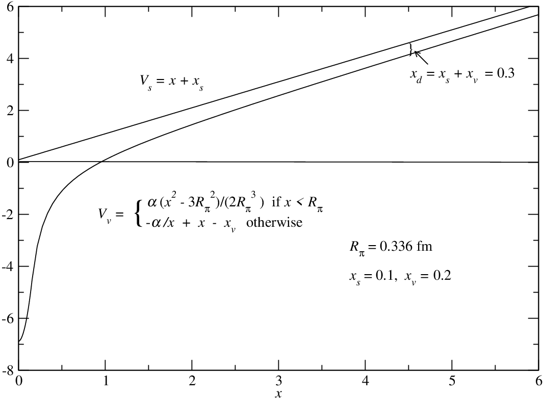
In this subsection we will assume both potentials and are linearly confining and have the same slopes (i.e., have the same string tension ). We assume the two potentials are displaced from each other with lying above , as in Fig. 19. That is, we assume
| (51) |
or, more appropriately, the smeared version of as described above in Sec. IV.1. Here and are parameters to be adjusted to get some desired eigenenergy. They give rise to a separation between the two asymptotic potentials of .
The reason for giving the potentials the same asymptotic slopes is to check that the spin-orbit interaction disappears as claimed in Ref. [25]. In doing so, we have changed the earlier offset of in to since, in GMSS (where only a Lorentz scalar potential was used), the negative offset represented a reasonable approximation the one-gluon-exchange attraction, roughly an average of the two potentials as shown in the figure.
Now, however, the BC’s at large distances are changed from those in Eq. (16), since, in the equation for , Eq. (7), the difference of the dimensionless and has its -dependence cancel. We need to solve the large- equations
| (52) |
from which
| (53) |
This is a minor modification of the differential equation for the Airy functions.[32] Since we require decaying solutions at our starting point for the inwards integrations, we discard the runaway solution for . The BC’s at large are then
| (54) |
Despite appearances, and still start off with the opposite slopes, as in Eq. (16), since, for , and .
For calculations, we simplified the displacement between the two potentials by setting , giving us one less parameter to worry about. The first wave function we want to compute is the ground state for the massless quark case, , starting out with and then adjusting both and until we get the desired eigenenergy, noted above in Eq. (31).
It turns out that to do so is trickier than in the -only case, presumably because of the cancellation between and in the differential equation for . Our first iterative search with found a highly excited state with , not the desired 0.7263, for which had six nodes! After some hand-searching on , we found we could get a ground state solution, i.e., a with no nodes, looking like the -quark of Fig. 7. This solution started with (very large!) and converged, in six iterations, to (about eight times too large).
From this solution we were able to march down, in small steps in (still with ), to , with the energy now smaller, , but still a factor of four too large. (For smaller values of the iterative procedure would not converge, with the matrix of Eq. (22) becoming singular.) The wave function for this solution was broader than that for the case, and the was relatively larger in comparison with .
At this point we began marching the value of in small steps up from zero, i.e., we began turning on the Coulomb attraction. As expected this attraction lowers the energy, and we were able to achieve the desired massless quark eigenenergy of 0.306 GeV with the following values:
| (55) |
The Long Marches did achieve the factor of eight reduction in the ground state eigenenergy. The wave functions for this massless quark solution are shown in Fig. 20. Note that here begins to resemble the hydrogen-atom ground state depicted by the dashed curve in Fig. 9, and it is much narrower than that shown in Fig. 3 .
The ground state solution says nothing about the PGG claim that, for and having equal slopes, the spin-orbit interaction vanishes. To check this we need to find, at a minimum, the eigenenergies of the and excited states. For the same values of and as in Eq. (55) and after some searching for good starting values for the iterative procedure, we obtained the three wave functions displayed in Figs. 21, 22, and 23. The wave functions here are narrower and more hydrogen-like than in the -only case (compare with Figs. 4, 5, and 6). The eigenenergies, in GeV, for these states are
| (56) |
The state is nearly degenerate with the state, some 200 MeV higher than in Sec. II.6, but this degeneracy is probably accidental. The real surprise here is the huge spin-orbit splitting between the and states, not what we expected from the claim made by PGG.[25]
This difference, it turns out, is due to the presence of the Coulomb attraction term in . If we set , then (again for ) we find the following eigenenergies (in GeV):
| (57) |
The wave functions in this case are similar to those in Figs. 21, 22, and 23 but are somewhat broader and less peaked near the origin. These results show the expected PGG symmetry (zero spin-orbit splitting). Note, incidentally, that the state is higher in energy than the states, as in the experimental charmonium spectrum.[26] One does conclude, however, that having a significant Coulomb contribution in will destroy the PGG symmetry.
V Summary
In this paper we have discussed, pedagogically, three increasingly more sensitive cases for solving the radial Dirac equations numerically:
- 1.
A Lorentz scalar potential, , which is linearly confining for quarks. The case of massless quarks is necessarily relativistic. As the mass of the quark increases, the wave function solutions become more and more n0n-relativistic.
- 2.
A Lorentz vector potential, , whose time-like component is a Coulomb potential. We first treated, numerically, the hydrogen atom, which is basically non-relativistic problem. We do, however, obtain the relativistic spin-orbit splitting between the and states (at the edge of our machine precision).
- 3.
The combination of scalar and vector potentials, aiming at a relativistic quark model of mesons. Of particular interest is when we do (and do not) get a relativistic spin-orbit splitting.
We thank L. J. Curtis, J. L. Friar, C. J. Fontes, M. D. Scadron, and R. Sharma for discussions and comments on this work.
References
- [1] P. A. M. Dirac, Proc. Roy. Soc. (London), A117, 610 (1928) and A118, 351 (1928).
- [2] C. E. DeTar, J. F. Donoghue, Bag Models Of Hadrons, Ann. Rev. Nucl. Part. Sci., 235-264 (1983).
- [3] A. W. Thomas, S. Teberge, and G. A. Miller, Phys. Rev. D 24, 216 (1981); D. B. Leinweber, A. W. Thomas, and R. D. Young, Phys. Rev. Lett. 86, 5011 (2001).
- [4] T. Goldman, K. R. Maltman, G. J. Stephenson, Jr., and K. E. Schmidt, Nucl. Phys. A481, 621 (1988). This reference is henceforth abbreviated as GMSS.
- [5] K. Saito and A. W. Thomas, Phys. Lett. B 327, 9 (1994); P. A. M. Guichon, K. Saito, E. N. Rodionov, and A. W. Thomas, Nucl. Phys. A̱ 601, 349 (1996).
- [6] E. E. Eichten et al., Phys. Rev. Lett. 34, 369 (1975); Phys. Rev. D 17, 3090 (1978); Phys. Rev. D 21, 203 (1980).
- [7] L. L. Foldy and S. A. Wouthuysen, Phys. Rev. 78, 29 (1950).
- [8] C. Darwin, Proc. Roy. Soc. (London), A118, 654 (1928).
- [9] H. A. Bethe and E. E. Salpeter, Quantum Mechanics of One- and Two-Electron Atoms (Springer, Berlin, 1957), Sec. 14.
- [10] See, e.g., C. K. Au and G. W. Rogers, Phys. Rev. A 22, 1820 (1980). It was on finding this paper that we were reminded of the coupled first-order radial Dirac equations.
- [11] See, e.g., Muonic Atoms and Molecules, ed. by L. A. Schaller and C. Petitjean (Birkhauser, Basel, 1993).
- [12] J. D. Bjorken and S. D. Drell, Relativistic Quantum Mechanics, (McGraw-Hill, New York, 1964), p. 55.
- [13] T. Goldman and R. R. Silbar, Phys. Rev. C 77, 865203 (2008).
- [14] M. Paris, Phys. Rev. C 68, 025201(2003).
- [15] A. Soares de Castro and J. Franklin, Int. J. Mod. Phys. A 15, 4355 (2000)
- [16] For the case when , see C. L. Critchfield, Phys. Rev. D 12, 923 (1975).
- [17] This interaction energy between two different quarks often goes by the name “color magnetic interaction,” which is essentially a hyperfine-like matrix element involving the coupling between the two quark’s spins. T. Goldman and R. R. Silbar, talk at the April APS Meeting, 2008, Denver CO.
- [18] E.g., George E. Forsythe, Michael A. Malcolm, and Cleve B. Moler. Computer Methods for Mathematical Computations, (Englewood Cliffs, NJ: Prentice-Hall, 1977). See Chapter 6.
- [19]
Mathematica is a software product of Wolfram Research,
http:\\www.wolfram.com, and its use is described by S. Wolfram in The Mathematica Book, 4th ed. (Cambridge University Press, Cambridge, 1999). - [20] http://t16web.lanl.gov/Silbar/.
- [21] In more usual units, = 0.19732 GeV-fm, which can be used for converting from 1/fm to GeV.
- [22] T. Goldman and R. R. Silbar, “ Mesons in a Relativistic Model”, in preparation.
- [23] B. D. Serot and J. D. Walecka, Advances in Nuclear Physics, ed. by J. W. Negele and E. Vogt (Plenum, New York, 1986), Vol. 16, p. 1.
- [24] N. Isgur, Phys. Rev. D 62. 054026 (2000); Phys. Rev. D 62. 014025 (2000).
- [25] P. R. Page, T. Goldman, and J. N. Ginocchio, Phys. Rev. Lett. 86, 204 (2001).
- [26] C. Amsler et al. (Particle Data Group), Phys. Lett. B667, 586 (2008).
- [27] See, e.g., R. Eisberg and R. Resnick, Quantum Physics of Atoms, Molecules, Solids, Nuclei, and Particles, (J. Wiley & Sons, New York, 1974), Chap. 8, pp. 310-311.
- [28] O. Klein, Z. Physik, 53, 157 (1929).
- [29] A. Calogeracos and N. Dombey, History and Physics of the Klein Paradox, Contemp. Phys. 40, 313 (1999)
- [30] See, e.g., R. Evans, The Atomic Nucleus, (McGraw-Hill, New York, 1955), Chap. 2.
- [31] M. Gell-Mann, R. Oakes, and B. Renner, Phys. Rev. 175, 2195 (1968). See also H. G. Dosch and S. Narison, Phys. Lett. B417, 173 (1998) and M. Jamin, Phys. Lett. B538, 71 (2002).
- [32] M. Abramovitz and I. A. Stegun, Handbook of Mathematical Functions, (Dover, New York, 1965), p. 446.




| Ry | (numerical) | (analytic) | |
|---|---|---|---|
| 10 | 1.360 | 1.3624 | 1.3624 |
| 100 | 136.0 | 161.6 | 161.6 |
| 136 | 251.546 | 433.8 | 448.3 |
| Point Coulomb | Smeared Coulomb | |||
|---|---|---|---|---|
| (GeV) | (GeV) | |||
| 0.0 | 0.306 | 0.195 | 0.306 | 0.195 |
| 0.2 | 0.251 | 0.244 | 0.251 | 0.237 |
| 0.4 | 0.194 | 0.343 | 0.194 | 0.305 |
| 0.6 | 0.135 | 0.551 | 0.135 | 0.417 |
| 0.8 | 0.072 | 1.052 | 0.074 | 0.611 |
| 1.0 | 0.004 | 2.653 | 0.007 | 0.977 |
| 1.2 | -.089 | 13.46 | -.156 | 1.759 |