Circuit partitions and $\#P$-complete products of inner products

Let $x,y\in\mathbb{C}^{k}$ be $k$-dimensional complex-valued vectors. We denote their inner product as

Now suppose we have a directed graph $G=(V,E)$. Let us associate a vector $x_{v}\in\mathbb{C}^{k}$ with each vertex $v$, and consider the product over all edges $(u,v)$ of the inner products of the corresponding vectors:

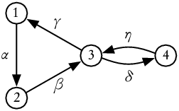
For instance, for the graph in Figure 1 this product is

The expectation of this product, where each $x_{v}$ is chosen independently and uniformly from the set of vectors in $\mathbb{C}^{k}$ of norm $1$, is a type of moment, where each $x_{v}$ appears with order $d^{\rm in}_{v}+d^{\rm out}_{v}$. It is a function of the graph $G$ and the dimension $k$, which we denote as follows:

A simple observation is that $q(G;k)$ is zero unless $G$ is Eulerian—that is, unless $d^{\rm in}_{v}=d^{\rm out}_{v}$ for each vertex $v$. Since $x_{v}$ appears in the product $d^{\rm in}_{v}$ times unconjugated and $d^{\rm out}_{v}$ times conjugated, multiplying $x_{v}$ by ${\rm e}^{i\theta}$ multiplies $q(G;k)$ by ${\rm e}^{i\theta(d^{\rm in}_{v}-d^{\rm out}_{v})}$. But multiplying by a phase preserves the uniform measure, so the expectation is zero if $d^{\rm in}_{v}\neq d^{\rm out}_{v}$ for any $v$.

So, let us suppose that $G$ is Eulerian. In that case, what is $q(G;k)$? Does it have a combinatorial interpretation? And how difficult is it to calculate? Our main result is this:

Our proof is very simple; we show that $q(G;k)$ is essentially identical to an existing graph polynomial, which is known to be $\#P$-hard to compute. Along the way, we will meet some nice combinatorics, and glancingly employ the representation theory of the unitary and orthogonal groups.

A circuit partition of $G$ is a partition of $G$’s edges into circuits. Let $r_{t}$ denote the number of circuit partitions containing $t$ circuits; for instance, $r_{1}$ is the number of Eulerian circuits. The circuit partition polynomial $j(G;z)$ is the generating function

For instance, for the graph in Figure 1 we have $j(G;z)=z+z^{2}$. This polynomial was first studied by Martin [10], with a slightly different parametrization; see also [1, 3, 4, 6, 9, 11, 12].

Now consider the following theorem.

Next we show that the cycle partition polynomial is $\#P$-hard. To our knowledge, the following theorem first appeared in [7]; we prove it here for completeness.

We can also consider the case where the $x_{v}$ are real-valued, and are chosen uniformly from the set of vectors in $\mathbb{R}^{k}$ of norm $1$. In this case, the inner product $\left\langle x_{u},x_{v}\right\rangle$ becomes symmetric, so the graph $G$ becomes undirected. We might then expect $q(G;k)$ to be related to the circuit partition polynomial for undirected circuits, and indeed this is the case.

We again wish to compute the tensor $X_{d}=\mathop{\mathrm{}}{Exp}_{x}\left|x^{\otimes d}\right\rangle\left\langle x^{\otimes d}\right|$. First, let $M_{d}$ denote the set of perfect matchings of $2d$ objects; note that

We can identify each matching $\mu\in M_{d}$ with a linear operator on $(\mathbb{R}^{k})^{\otimes d}$, where the first $d$ objects correspond to upper indices, and the last $d$ correspond to lower indices. However, in addition to permutations that wire upper indices to lower ones with a bipartite matching, we now also have “cups” and “caps” that wire two upper indices, or two lower indices, to each other. For instance, if $d=2$ then $M_{d}$ includes three operators, corresponding to the three perfect matchings of $4$ objects:

$$\delta^{\alpha_{1}}_{\beta_{1}}\delta^{\alpha_{2}}_{\beta_{2}}=\raisebox{-7.0pt}{\includegraphics[height=18.0pt]{identity}}\,,\quad\delta^{\alpha_{1}}_{\beta_{2}}\delta^{\alpha_{2}}_{\beta_{1}}=\raisebox{-7.0pt}{\includegraphics[height=18.0pt]{exchange}}\,,\quad\mbox{and}\quad\delta^{\alpha_{1},\alpha_{2}}\delta_{\beta_{1},\beta_{2}}=\raisebox{-7.0pt}{\includegraphics[height=18.0pt]{cupcap}}\,.$$

(12)

The first two of these operators correspond to the identity permutation and the transposition $\tau_{1,2}$ respectively, as in the previous section. The third one is a cupcap; it is the outer product of the vector $\sum_{i=1}^{k}e_{i}\otimes e_{i}$ with itself, where $e_{i}$ denotes the $i$th basis vector in $\mathbb{R}^{k}$. We denote it $\gamma_{1,2}$, and more generally $\gamma_{ij}=\delta^{\alpha_{i},\alpha_{j}}\delta_{\beta_{i},\beta_{j}}$.

Now, in the real-valued case, Lemma 1 becomes the following:

As before, $q(G;k)$ is a contraction of the tensors $X_{d}$. However, now $G$ is undirected, with no distinction between incoming and outgoing edges, so at each vertex of degree $d_{v}$ the appropriate tensor is $X_{d_{v}/2}$. Applying Lemma 2 to each $v$ sums over all the ways to match $v$’s edges with each other, and hence sums over all possible partitions of $G$’s edges into undirected cycles. The trace of the resulting diagram is again the number of ways to label each cycle with a basis vector. So, if define a polynomial $j_{\rm undirected}(G;z)$ as $\sum_{t=1}^{\infty}r_{t}z^{t}$, where $r_{t}$ is the number of partitions with $t$ cycles, then Theorem 2 becomes

Our results above assume that each $x_{v}$ is chosen uniformly from the set of vectors in $\mathbb{C}^{k}$ or $\mathbb{R}^{k}$ of norm $1$. Another natural measure would be to choose each component of $x_{v}$ independently from the Gaussian distribution with variance $1/k$, so that $\mathop{\mathrm{}}{Exp}[\left|x_{v}\right|^{2}]=1$.

For vectors in $\mathbb{C}^{k}$, the probability density of the norm $\left|x\right|$ is then

Compared to the case where $\left|x_{v}\right|=1$, each $x_{v}$ contributes scaling factor of $\left|x_{v}\right|^{2d}$ to the product (1). The even moments of (16) are

so in the Gaussian distribution (4) becomes

where $m$ denotes the number of edges.

We could also have derived this directly from the Gaussian analog of Lemma 1. If $x$ is chosen according to the Gaussian distribution on $\mathbb{C}^{k}$, and we again let $X_{d}$ denote $\mathop{\mathrm{}}{Exp}_{x}\left|x^{\otimes d}\right\rangle\left\langle x^{\otimes d}\right|$, then

Similarly, in the real-valued case, if we choose each component of $x\in\mathbb{R}^{k}$ from the Gaussian distribution on $\mathbb{R}$ with variance $1/k$, then (15) becomes

since

Both (18) and (20) are consequences of Wick’s Theorem [8, 15], that if $x_{1},\ldots,x_{2t}$ obey a multivariate Gaussian distribution with mean zero, then

References

- [1] R. Arratia, B. Bollobás, and G. Sorkin, The interlace polynomial: A new graph polynomial. Proc. 11th Annual ACM-SIAM Symposium on Discrete Algorithms 237–245 (2000).
- [2] Andrea Austin, The Circuit Partition Polynomial with Applications and Relation to the Tutte and Interlace Polynomials. Rose-Hulman Undergraduate Mathematics Journal, 8(2) (2007).
- [3] Béla Bollobás, Evaluations of the Circuit Partition Polynomial. Journal of Combinatorial Theory, Series B 85, 261–268 (2002)
- [4] André Bouchet, Tutte-Martin polynomials and orienting vectors of isotropic systems. Graphs Combin. 7(3) 235–252 (1991).
- [5] Richard Brauer, On Algebras Which are Connected with the Semisimple Continuous Groups. Annals of Mathematics, 38(4) 857–872 (1937).
- [6] Joanna A. Ellis-Monaghan, New results for the Martin polynomial. Journal of Combinatorial Theory, Series B 74, 326–352 (1998).
- [7] Joanna A. Ellis-Monaghan and Irasema Sarmiento, Distance hereditary graphs and the interlace polynomial. Combinatorics, Probability and Computing 16(6) 947–973 (2007).
- [8] L. Isserlis, On a formula for the product-moment coefficient of any order of a normal frequency distribution in any number of variables. Biometrika 12: 134–139 (1918).
- [9] F. Jaeger, On Tutte polynomials and cycles of plane graphs. Journal of Combinatorial Theory, Series B 44, 127–146 (1988).
- [10] P. Martin, Enumérations eulériennes dans les multigraphes et invariants de Tutte-Grothendieck. Thesis, Grenoble 1977.
- [11] Michel Las Vergnas, On Eulerian partitions of graphs. Research Notes in Mathematics 34, 62–75 (1979).
- [12] Michel Las Vergnas, On the evaluation at of the Tutte polynomial of a graph. Journal of Combinatorial Theory, Series B 44, 367–372 (1988).
- [13] Dirk Vertigan, The Computational Complexity of Tutte Invariants for Planar Graphs. SIAM J. Comput., 35(3) 690–712 (2006).
- [14] Hans Wenzl, On the Structure of Brauer’s Centralizer Algebras. Annals of Mathematics 128(1) 173–193 (1988).
- [15] Gian-Carlo Wick, The evaluation of the collision matrix. Physical Review 80(2): 268–272 (1950).