Probing the dynamical behavior of dark energy
Abstract
We investigate dynamical behavior of the equation of state of dark energy by employing the linear-spline method in the region of low redshifts from observational data (SnIa, BAO, CMB and 12 data). The redshift is binned and is approximated by a linear expansion of redshift in each bin. We leave the divided points of redshift bins as free parameters of the model, the best-fitted values of divided points will represent the turning positions of where changes its evolving direction significantly (if there exist such turnings in our considered region). These turning points are natural divided points of redshift bins, and between two nearby divided points can be well approximated by a linear expansion of redshift. We find two turning points of in and one turning point in , and could be oscillating around . Moreover, we find that there is a deviation of from around in both correlated and uncorrelated estimates.
pacs
98.80.Es, 95.36.+x, 98.80.-kI Introduction
It has been more than ten years since our universe was found to be in accelerating expansion [1]. A dominated and uniformly distributed energy component of the universe, called dark energy (DE), should be responsible for the acceleration. Many DE models have been proposed [2, 3, 4, 5, 6]. The simplest cosmological model is CDM model, which contains a cosmological constant as dark energy. While CDM model is still consistent well with all observational data, a lot of efforts have been made to find out whether DE is time-evolving or is just the cosmological constant. To do that, several parameterizations of equation of state (EoS) of DE have been proposed to fit with observational data, such as the ansatz [7], the EoS expanded by redshift, and the CPL parametrization [8, 9] , expanded by scale factor. Both of them contain two free parameters: , the present value of EoS, and or , represents the time evolution of EoS. Clearly, constraints of EoS obtained by using these parameterizations are model-dependent. Given an unreal assumption of EoS of DE, one may lead to wrong conclusions. Some model-independent methods have also been proposed [10, 11, 12, 13], such as the widely-used uncorrelated bandpower estimates (UBE) [11, 14], in which the redshift is binned and is assumed as a constant in each redshift bin. Note that the UBE method just approximates the actual by an averaged constant in each bin if DE is dynamical. If there are sufficient data, can be accurately reconstructed. However, current data could only support a few bins, thus UBE is always used to test the deviation of from the cosmological constant and used as a supplementary for the parameterizations of . Note that the cubic-spline interpolation has also been proposed to study the binned [15, 16]. However, no convincing evidence of dynamic DE has been found [15, 16, 17]. In addition, let us note that the ansatz, , of redshift expansion and CPL parametrization exclude the possibility of an oscillation EoS, if they are used to fit the whole expansion history of the universe. While the UBE method needs enough bins to reveal the real dynamical behavior of DE, the errors will get larger as the number of bins increases.
In this paper, we would like to probe the dynamical behavior of by using the linear-spline method. We will approximate in each redshift bin by a linear function , and require that is continuous in the region under consideration. Since most of data we used (e.g., SnIa data) are in low redshift, we will focus on the region of low redshift, such as and . In such regions, the width of each redshift bin is small and the linear expansion could be a better approximation of than a constant in each bin. When fitting with the observational data, we leave the divided positions of bins as free parameters. Since the linear function is monotonic, the best-fitted can represent the turning points of , where is not linear enough or even non-monotonic (i.e., where departs from zero substantially). Actually we do find some turning points of from observational data, and the constructed just turns its evolution direction at the best-fitted positions of . In this way, we only need to divide redshift into a few bins, the turning points are natural divided points of redshift and between two nearby points can be accurately reconstructed by linear expansion. Compared to the cubic-spline method, the linear-spline (LS) method can find turning locations of more accurately and reduce the errors due to less the number of bins. The LS method is also nearly model-independent, like the piecewise constant and cubic-spline method. Replacing the linear expansion by CPL parametrization in each bin, we have reached the almost same results.
For the current status of observational data, LS method may be more suitable to study than the piecewise constant and the cubic spline method. If DE is dynamical or even oscillating, by using the LS method it should be more possible to find deviations from the cosmological constant, at the turning points the deviation from should be more explicit. If DE is just the cosmological constant, it seems more confident if the best-fitted linear expansions construct an line, while the oscillation of around could disappear by averaging with the piecewise constant method. Compared to the piecewise constant case, the only price we pay is that there is one more parameter in the LS method if the number of bins is the same in two cases. Compared to the cubic spline method, the form of in each bin only depends on values of at two boundaries, thus the parameters in will not be heavily correlated. Furthermore, the cubic-spline method seems not suitable for finding the turning points of . In all, the LS method could reconstruct explicitly by using the least number of bins, and errors of the parameters from observational data will be small, compared to the case with more bins.
The paper is organized as follows. In section II we introduce in detail the method we will use and construct corresponding cosmological models. In section III, we show how to fit our model with 397 Constitution SnIa sample [18], BAO data from SDSS DR7 [19], CMB datapoints () from WMAP5 [20] and 12 Hubble evolution data [21, 22]. The fitting results are presented in section IV. We give our conclusions and discussions in section V.
II Methodology
To fit models with observational data, we need to know the form of Hubble function (or ). In a flat FRW universe
| (1) |
where , , and are present values of the dimensionless energy density for radiations, baryons, dark matter and dark energy, respectively, and . The energy densities of baryons and dark matter are always written together as . The radiation density is the sum of photons and relativistic neutrinos [20]:
where is the number of neutrino species and for (). The evolving function for DE depends on :
| (2) |
For example,
for the CPL parametrization and for , respectively. Here we divide into bins and assume in the first bins as
| (3) |
and require to be continuous at divided points:
| (4) |
Note that here prime does not represent a derivative, instead is just the slope of the linear expansion in the bin. Thus the independent parameters are
| (5) |
where the total number of parameters is with . Alternatively, we can express as
| (6) |
Now the parameters become ’s, which are values of at the divided points and boundaries . In this case we have
| (7) | |||||
where we have used . For in the last bin , we set it to be a constant , and
| (8) |
Now the formula for is ready.
There is one more thing to be mentioned: once we have fitted our model with the data introduced in the next section, errors of are correlated, i.e., the errors of are dependent on each other. New parameters can be defined by transforming the covariance matrix of , so that errors of new parameters are decorrelated and do not entangle with each other. The new uncorrelated parameters are referred to as the principal components [10, 23], and they are directly related to their own locations (unlike the correlated case). So errors of the uncorrelated parameters are more interpretable and meaningful. For more discussions and implications of the uncorrelated parameters, we refer to the references [11, 14, 24]. In section IV, we will show both errors of correlated and uncorrelated parameters of . The uncorrelated technique we adopt from [11] is as follows.
1. Get the covariance matrix
| (9) |
where is the vector of . The Fisher matrix F is defined by .
2. Diagonalize the Fisher matrix by an orthogonal matrix O
| (10) |
where is diagonal.
3. Define a new matrix as
| (11) |
and normalize so that the sum of its each row is equal to .
4. Define new parameters by , where are components of the vector .
Clearly for the case of (i.e., the cosmological constant case), we will have . The covariance of new parameters is
| (12) |
In this way the errors of the new parameters become uncorrelated.
The uncorrelated parameters are linear combinations of , and the coefficients are just row elements of . The transformation matrix constructed in this method ensures that most of the coefficients are positive. So most of coefficients are in . In this way, the original correlated parameters are weight-averaged, which leads to the uncorrelated parameters . As a result, if is of the quintom form, the uncorrelated always looks more consistent with the cosmological constant than the correlated one.
III Sets of Observational data
We will fit our model by employing some observational data including SnIa, BAO, CMB and Hubble evolution data. The data for SnIa are the 397 Constitution sample [18]. for SnIa is obtained by comparing theoretical distance modulus ( ) with observed of supernovae:
| (13) |
To reduce the effect of , we expand with respect to [25]:
| (14) |
where
| (15) |
Eq. (14) has a minimum as
which is independent of . In fact, it is equivalent to performing an uniform marginalization over , the difference between and the marginalized is just a constant [25]. We will adopt as the chi-square between theoretical model and SnIa data.
We will also use the Baryon Acoustic Oscillations (BAO) data from SDSS DR7 [19], the datapoints are
| (16) |
and
| (17) |
where is the comoving sound horizon at the baryon drag epoch [26], and
| (18) |
encodes the visual distortion of a spherical object due to the non Euclidianity of a FRW space-time.
The CMB datapoints we will use are () from WMAP5 [20]. is the redshift of recombination [28], is the scaled distance to recombination
| (19) |
and is the angular scale of the sound horizon at recombination
| (20) |
where is the comoving distance and is the comoving sound horizon at recombination
| (21) |
where the sound speed and is the photon-baryon energy density ratio.
The of the CMB data is constructed as:
| (22) |
where
and the inverse covariance matrix
The fourth set of observational data is Hubble evolution data from [21] and [22], its is defined as
| (31) |
Note that redshifts of these data fall in the region .
In summary,
| (32) |
IV Fitting Results

IV.1 Model I
| Models | |||||
|---|---|---|---|---|---|
| Model I | 459.728 | 0.204 | 1.494 | 5.983 | 467.409 |
| CPL | 465.621 | 0.251 | 1.716 | 10.818 | 478.406 |
| CDM | 465.759 | 1.014 | 1.470 | 10.850 | 479.093 |
At first, we divide the whole region of redshift into bins (i.e., ), the divided points and boundaries are , where and are left as free parameters of the model, and . In the fourth bin we set . It means that we divide the region with into bins and seek for two possible turning points of in this region. The reconstructed of the best-fitted model is shown in Fig. 1, which indicates that there exist (at least) two turning points of in and the best-fitted values and . Here for the best-fitted parameters, roughly speaking it is a good improvement, compared with the corresponding for the best-fitted CPL model and for the CDM model. As shown in Table I, this improvement of is mainly due to the decrease of and . It is not surprising, as redshifts of the two data sets are distributed in whole range of , while the BAO data are in the region and the CMB data are in the region . The result implies that these two data sets are quite favor of turnings of around and respectively. This result is consistent with recent UBE of [27]. While in CPL and CDM models it is impossible to have such turnings of , which leads to the big differences between of Model I and that of CDM and CPL models. This result also implies that there exists the possibility with an oscillating EoS. Note that the error bar of in the third bin is larger than those in the first two bins because there are much less data points.
We have also divided the region of into 4 bins, and found that there is almost no improvement of compared to the case of 3 bins, which indicates there is no more turning points of in this region.
| parameters | ||||||||||
|---|---|---|---|---|---|---|---|---|---|---|
| best-fitted values | 0.688 | 0.049 | 0.279 | 0.44 | 1.07 | -0.63 | -1.57 | 2.28 | -16.84 | {-1} |
IV.2 Model II
As data points with are rather less than those with , to see clearly the evolution behavior of EoS in the region of low redshift, we now focus on the region with , avoiding the possible turning point around , and set the divided points as: , i.e.,
In this case, we obtain the best-fitted tuning point , and the best-fitted is shown in Fig. 1 (the red, dashed line) which almost coincides with the best-fitted of Model I in . This indicates that the data favor to turn its evolution direction around , and favor an EoS with crossing the cosmological constant () [29]. Then we obtain and errors of parameters by using the MCMC method. Here we have fixed in the process to obtain the errors of the parameters. Note that the errors of the parameters also represent errors of whole in each bin, the and errors of shown in Fig. 2 are obtained by connecting the corresponding error ranges of . If another parameter set of (as introduced in section II) was used, one will get the same result as that of Fig. 2.
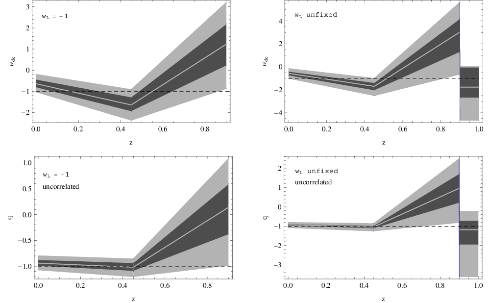
We see from the top left panel of Fig. 2 that there are deviations of from around and beyond , and around the deviation is beyond . We decorrelate the parameters in by using the technique introduced in section II. The uncorrelated errors are shown in the bottom left panel of Fig. 2. In that case, there are no more explicit deviations from around and , however, there is still a deviation from around .

One may suspect that the explicit derivations are caused due to the fact that we have fixed the value of as in the third bin. To check this, we consider the case with a floating . Two right panels of Fig. 2 show the correlated and uncorrelated results for the case with the floating . We see that in this case, there is even larger deviation from around . We have also used the CPL parametrization to replace the linear expansion in each bin, and found that the errors are almost the same as those in the case of the linear expansion and there is still a deviation of from around . We will extend our discussion of this result in the last section. In Fig. 3 we plot the likelihoods and weight functions of the uncorrelated parameters . The weight functions are constructed from the transformation matrix U, which show how uncorrelated parameters are determined. It is shown that the parameters of are less correlated than that of the cubic-spline case [16].
| parameters | ||||||||
|---|---|---|---|---|---|---|---|---|
| best-fitted values | 0.684 | 0.050 | 0.282 | 0.45 | -0.63 | -1.59 | 1.24 | {-1} |
| ML and 2 errors | {0.45} | {-1} | ||||||
| best-fitted values | 0.687 | 0.049 | 0.280 | {0.45} | -0.59 | -1.69 | 2.54 | -1.72 |
| ML and 2 errors |
We have also divided into three bins, to see whether there exist two turning points of in this region. We found that with the additional parameters ( and ), there is almost no improvement of , compared to the bins case (Model II). This indicates that there is no more turning points and can be well approximated by just two linear expansions in the region . Of course, there is another possibility that the current data are not enough to find out more turning points.
V Conclusions and Discussions
In this paper we have investigated the dynamical behavior of the EoS of DE in the region of low redshift in a nearly model-independent way. The redshift in that region is binned and in each bin is approximated by a linear expansion of redshift , and in the large redshift region we set to be a constant . While fitting the model with some observational data which include SnIa, BAO, CMB and Hubble evolution data, we leave the divided points of bins as free parameters. If the evolution of is not monotonous, or is not linear enough in the region under consideration, the best-fitted divided points will represent the turning points, where changes its evolving direction significantly. In this way we can explicitly reconstruct by using a few bins, and the errors of parameters from observational data will be small due to the small number of bins. First we have tried to find the turning points within the region of redshift , and set in the region (Model I). Our results show that the data favor two turning points of in , and may have an oscillation form [30]. Our results are consistent with those by the UBE method in [27].
Since the main data points are in and our result in Model I shows there may be a turning point around , to see clearly the dynamical behavior of EoS in that region, we have focused on the region in Model II. We have found one turning point only in , the reconstructed in the best-fitted model is almost the same as that reconstructed in Model I in . We have also obtained the errors of at and in . In both correlated and uncorrelated estimates with a fixed or a floating constant , we found that there is a deviation of from around .
It is interesting to see whether the deviation of EoS from around is physical, or is caused by some unknown technical causes in fitting. If it is physical, it then clearly shows that DE is dynamical. But in UBE of there seems no such distinct deviation around , it may be due to the difference between the discontinuity of in the piecewise constant case and the continuity in LS case [31]. In [16], where the cubic-spline method is used, there is also no such an explicit deviation around , but it is likely due to its set of EoS in the last bin : to fit well with the data of , should be much minus, which would suppress the reconstructed around . Of course, it is also possible that such a big deviation around is due to the non-smoothness of at the divided points in our LS method. In the LS method, is continuous, but not smooth at the divided points, i.e., its derivative is not continuous at those points. In fact, in LS method can be made smooth at the divided points, such as by the relation
| (37) |
where is the slope of linear expansion in the bin ( and ), and is related to the smoothed extent at the divided points. With this parameterization, one can still find out the turning positions of that are favored by observational data, and perturbations of DE can be calculated.
Furthermore our results are also dependent on the data set we have used [32]. For example, although there is still a deviation at by using the widely-used data set SnIa + CMB-shift R + BAO parameter A [33], now the best-fitted turning point in changes to . Whatever, from the observational data we have used, a big deviation of from around is found. Unlike the deviations around and , this deviation around does not to be reduced in the uncorrelated estimate. At least, our result shows that if DE is dynamical it is more possible to find the deviation of from around this redshift value.
If the EoS of DE is indeed of an oscillating behavior around , it is then not surprising that the cosmological constant always fits well with observational data because the oscillating behavior could be smeared in the luminosity distance. However, if the oscillation region of is wide enough (like the case of our best-fitted in Model I), DE may be distinguished confidently from the cosmological constant by more precise astronomical observations in the next generation. In addition, let us mention that an oscillating behavior of is also possibly due to some systematic errors in observational data, or due to some interactions between DE and dark matter [34].
Acknowledgments
RGC thanks Y.G. Gong and B. Wang for some relevant discussions. This work was partially supported by NNSF of China (No. 10821504 and No. 10975168) and the National Basic Research Program of China under grant 2010CB833000.
References
- [1] A. G. Riess et al. [Supernova Search Team Collaboration], Astron. J. 116, 1009 (1998) [arXiv:astro-ph/9805201]; S. Perlmutter et al. [Supernova Cosmology Project Collaboration], Astrophys. J. 517, 565 (1999) [arXiv:astro-ph/9812133].
- [2] E. J. Copeland, M. Sami and S. Tsujikawa, Int. J. Mod. Phys. D 15, 1753 (2006) [arXiv:hep-th/0603057].
- [3] R. R. Caldwell and P. J. Steinhardt, Phys. Rev. D 57, 6057 (1998) [arXiv:astro-ph/9710062].
- [4] P. J. Steinhardt, L. M. Wang and I. Zlatev, Phys. Rev. D 59, 123504 (1999) [arXiv:astro-ph/9812313].
- [5] S. Capozziello, S. Carloni and A. Troisi, Recent Res. Dev. Astron. Astrophys. 1, 625 (2003) [arXiv:astro-ph/0303041].
- [6] M. Li, Phys. Lett. B 603, 1 (2004) [arXiv:hep-th/0403127]; R. G. Cai, Phys. Lett. B 657, 228 (2007) [arXiv:0707.4049 [hep-th]]; H. Wei and R. G. Cai, Phys. Lett. B 660, 113 (2008) [arXiv:0708.0884 [astro-ph]]. B. Feng, X. L. Wang and X. M. Zhang, Phys. Lett. B 607, 35 (2005) [arXiv:astro-ph/0404224]; C. Gao, X. Chen and Y. G. Shen, Phys. Rev. D 79, 043511 (2009) [arXiv:0712.1394 [astro-ph]].
- [7] D. Huterer and M. S. Turner, Phys. Rev. D 64, 123527 (2001) [arXiv:astro-ph/0012510]; A. R. Cooray and D. Huterer, Astrophys. J. 513, L95 (1999) [arXiv:astro-ph/9901097]; D. Huterer and M. S. Turner, Phys. Rev. D 60, 081301 (1999) [arXiv:astro-ph/9808133]; J. Weller and A. J. Albrecht, Phys. Rev. Lett. 86, 1939 (2001) [arXiv:astro-ph/0008314].
- [8] M. Chevallier and D. Polarski, Int. J. Mod. Phys. D 10, 213 (2001) [arXiv:gr-qc/0009008].
- [9] E. V. Linder, Phys. Rev. Lett. 90, 091301 (2003) [arXiv:astro-ph/0208512].
- [10] D. Huterer and G. Starkman, Phys. Rev. Lett. 90, 031301 (2003) [arXiv:astro-ph/0207517].
- [11] D. Huterer and A. Cooray, Phys. Rev. D 71, 023506 (2005) [arXiv:astro-ph/0404062].
- [12] A. Hojjati, L. Pogosian and G. B. Zhao, arXiv:0912.4843 [astro-ph.CO].
- [13] Y. Wang, Phys. Rev. D 80, 123525 (2009) [arXiv:0910.2492 [astro-ph.CO]].
- [14] S. Sullivan, A. Cooray and D. E. Holz, JCAP 0709, 004 (2007) [arXiv:0706.3730 [astro-ph]].
- [15] G. B. Zhao, D. Huterer and X. Zhang, Phys. Rev. D 77, 121302 (2008) [arXiv:0712.2277 [astro-ph]].
- [16] P. Serra, A. Cooray, D. E. Holz, A. Melchiorri, S. Pandolfi and D. Sarkar, arXiv:0908.3186 [astro-ph.CO].
- [17] Y. Gong, R. G. Cai, Y. Chen and Z. H. Zhu, arXiv:0909.0596 [astro-ph.CO].
- [18] M. Hicken et al., Astrophys. J. 700, 331 (2009) [arXiv:0901.4787 [astro-ph.CO]].
- [19] W. J. Percival et al., arXiv:0907.1660 [astro-ph.CO].
- [20] E. Komatsu et al. [WMAP Collaboration], Astrophys. J. Suppl. 180, 330 (2009) [arXiv:0803.0547 [astro-ph]].
- [21] J. Simon, L. Verde and R. Jimenez, Phys. Rev. D 71, 123001 (2005) [arXiv:astro-ph/0412269].
- [22] E. Gaztanaga, A. Cabre and L. Hui, arXiv:0807.3551 [astro-ph].
- [23] A. J. S. Hamilton and M. Tegmark, Mon. Not. Roy. Astron. Soc. 312, 285 (2000) [arXiv:astro-ph/9905192].
- [24] R. de Putter and E. V. Linder, Astropart. Phys. 29, 424 (2008) [arXiv:0710.0373 [astro-ph]].
- [25] S. Nesseris and L. Perivolaropoulos, Phys. Rev. D 72, 123519 (2005) [arXiv:astro-ph/0511040].
- [26] D. J. Eisenstein and W. Hu, Astrophys. J. 496, 605 (1998) [arXiv:astro-ph/9709112].
- [27] Q. G. Huang, M. Li, X. D. Li and S. Wang, Phys. Rev. D 80, 083515 (2009) [arXiv:0905.0797 [astro-ph.CO]]; G. B. Zhao and X. Zhang, arXiv:0908.1568 [astro-ph.CO]; S. Qi, T. Lu and F. Y. Wang, arXiv:0904.2832 [astro-ph.CO].
- [28] W. Hu and N. Sugiyama, Astrophys. J. 471, 542 (1996) [arXiv:astro-ph/9510117].
- [29] H. Zhang, arXiv:0909.3013 [astro-ph.CO].
- [30] R. Lazkoz, S. Nesseris and L. Perivolaropoulos, JCAP 0511, 010 (2005) [arXiv:astro-ph/0503230]; M. X. Luo and Q. P. Su, Phys. Lett. B 626, 7 (2005) [arXiv:astro-ph/0506093].
- [31] In preparing.
- [32] J. C. B. Sanchez, S. Nesseris and L. Perivolaropoulos, JCAP 0911, 029 (2009) [arXiv:0908.2636 [astro-ph.CO]]; H. Wei, arXiv:0906.0828 [astro-ph.CO]; Y. Gong, B. Wang and R. G. Cai, arXiv:1001.0807 [astro-ph.CO].
- [33] D. J. Eisenstein et al. [SDSS Collaboration], Astrophys. J. 633, 560 (2005) [arXiv:astro-ph/0501171].
- [34] J. H. He, B. Wang and P. Zhang, Phys. Rev. D 80, 063530 (2009) [arXiv:0906.0677 [gr-qc]]; R. G. Cai and Q. Su, arXiv:0912.1943 [astro-ph.CO]; C. Feng, B. Wang, E. Abdalla and R. K. Su, Phys. Lett. B 665, 111 (2008) [arXiv:0804.0110 [astro-ph]]; H. H. Xiong, Y. F. Cai, T. Qiu, Y. S. Piao and X. Zhang, Phys. Lett. B 666, 212 (2008) [arXiv:0805.0413 [astro-ph]].