INSTITUT NATIONAL DE RECHERCHE EN INFORMATIQUE ET EN AUTOMATIQUE
Towards a Generic Framework to Generate Explanatory Traces of Constraint Solving and Rule-Based Reasoning
Pierre Deransart --- Rafael Oliveira††footnotemark:
N° 7165
Decembre 2009
Towards a Generic Framework to Generate Explanatory Traces of Constraint Solving and Rule-Based Reasoning
Pierre Deransart, Rafael Oliveira00footnotemark: 0
Domaine : Algorithmique, programmation, logiciels et architectures
Équipes-Projets Contraintes
Rapport de recherche n° 7165 — Decembre 2009 — ?? pages
Abstract: In this report, we show how to use the Simple Fluent Calculus (SFC) to specify generic tracers, i.e. tracers which produce a generic trace. A generic trace is a trace which can be produced by different implementations of a software component and used independently from the traced component.
This approach is used to define a method for extending a java based CHR∨ platform called CHROME (Constraint Handling Rule Online Model-driven Engine) with an extensible generic tracer. The method includes a tracer specification in SFC, a methodology to extend it, and the way to integrate it with CHROME, resulting in the platform CHROME-REF (for Reasoning Explanation Facilities), which is a constraint solving and rule based reasoning engine with explanatory traces.
Key-words: Trace, CHR, CHR∨, CHROME, CHROME-REF, Tracer, Meta-Theory, Model Driven Engineering, Tracer Driver, Analysis Tool, Program Analysis, Observational Semantics, Software Component, Debugging, Programming Environment, Logic Programming, Validation
Towards a Generic Framework to Generate Explanatory Traces of Constraint Solving and Rule-Based Reasoning
Résumé : Dans ce rapport, nous montrons comment utiliser le calcul des fluents simple (SFC) pour spécifier des traceurs génériques, c’est-à-dire qui produisent des traces génériques. Une trace générique est une trace qui peut être produite par différentes implémentations d’un composant logiciel et être utilisées indépendamment du composant tracé.
Cette approche est utilisée pour définir une méthode pour introduire dans une platforme CHR∨ basée Java et appelée CHROME (Constraint Handling Rule Online Model-driven Engine) un traceur générique extensible. La méthode comprend une spécification du traceur en SFC, une méthodologie d’extension, et leur implantation dans CHROME, afin d’obtenir la plateforme CHROME-REF (Raisonnement Explicatif Facilité), qui est un solveur de contraintes et moteur de raisonnement à base de règles avec des traces d’explications.
Mots-clés : trace, CHR, CHR∨, CHROME, CHROME-REF, MDE, traceur, méta-théorie, pilote de tracer, analyseur, outils d’analyse, analyse de programme, analyse dynamique, sémantique observationnelle, composant logiciel, déboggage, environnement de programmation, programmation en logique, validation
1 Introduction
In this report we define a method for extending a java based CHR∨11 1 CHR stands for Constraint Handling Rule [22], CHR∨ for CHR with disjunction. platform called CHROME (Constraint Handling Rule Online Model-driven Engine) with an extensible generic tracer. CHROME is presently developed at the Federal University of Pernambuc [56] with the purpose to allow the development of large software using CHR paradigm.
The method consists of firstly to build a formal specification of a tracer for CHR∨, the kernel of the system, and to extend it according to further CHR∨ extensions. The specification defines a generic trace which is as independent as possible from a particular CHR platform or specific usages. Then, secondly, it is suggested to use this specification as a guideline to extend the MDE scheme development of CHROME, with a tracer scheme development, resulting in the plateform CHROME-REF (REF stands for Reasoning Explanation Facilities), which is a constraint solving and rule based reasoning engine with explanatory traces.
This report is almost based on the internship work of R. Oliveira [38]. We introduce first some contextual aspects of this work.
1.1 The CHR World
The language CHR has matured over the last decade to a powerful and elegant general-purpose language with a wide spectrum of application domains [52]. The interest in CHR∨ stemmed from past research having shown that:
- •
CHR is simultaneously a Turing-complete declarative programming language and an expressive knowledge representation language with declarative formal semantics in classical first-order logic [22];
- •
- •
A CHR∨ inference engine can support an unmatched variety of practical automated reasoning tasks, including constraint solving with variables from arbitrary domains, satisfiability [22], entailment [50], abduction [1], agent action planning [50] and agent belief update [50] and revision [55]. In addition, it support several of these tasks under logical [50], plausibilistic [8] and probabilistic epistemological [42] assumptions. [10] adds default reasoning to this list, by showing how to represent default logic theories in CHRV. It also discusses how to leverage this representation together with the well-know correspondence between default logic and Negation As Failure (NAF) in logic programming, to propose an extension CHRV;naf of CHRV allowing NAF in the rule heads. And [20] adds concurrency.
The Figure 1 shows the several automatic reasoning services that are subsumed by CHR∨ and extensions.

For all its above strengths, CHR remained until recently a language for Knowledge Representation and Programming (KR&P) in-the-small mainly used to fast prototype intelligent, innovative systems. The ORCAS project 22 2 http://www.cin.ufpe.br/~jr/mysite/C4RBCPProject.html, constitutes a first and preliminary step towards the long term goal, to turn CHR into a platform for KR&P in-the-large industrial strength, operationally deployed systems. It addressed one key KR&P in-the-large requirement, namely rule base engineering scalability through rule base encapsulation and assembly in reusable software components.
1.2 From CHROME to CHROME-REF
CHROME stands for Constraint Handling Rule Online Model-driven Engine, is a model-driven, component-based, scalable, online, Java-hosted CHR∨ engine to lay at the bottom of the framework as the most widely reused automated reasoning component. The idea of CHROME is also to demonstrate how a standard set of languages and processes prescribed by MDA can be used to design concrete artefacts, such as: a versatile inference engine for CHR∨ and its compiler component that generates from a CHR∨ base the source code of Java classes.
The project CHROME-REF (Constraint Handling Rule Online Model-Driven Engine with Reasoning Explanation Facilities) constitutes a preliminary step, towards extending CHR and CHR engines with a formally founded, flexible and user-friendly reasoning explanation facility. The need for flexible and user-friendly explanatory reasoning tracing facilities for rule-based systems has been recognized since the initial success of production rule expert systems in the 80s. However, the expressive power of CHR being far superior than that of a mere production system, through the addition of functional terms, rewrite rules and backtracking search, makes debugging a CHR rule base also more complex than debugging a production rule base. In turn, this added complexity makes the need for sophisticated rule engine tracing facilities more crucial and the issues in their design and implementation more challenging.
This project is pioneering the investigation of these issues. CHROME assembles CHR base independent run-time components for constraint store management, fired ruled history management, constraint entailment, query processing and intelligent search, with optimized components resulting from the compilation of the CHR base. Following the KobrA2 model-driven, component-based, orthographic software engineering method [4, 5], CHROME was built by first specifying a refined Platform-Independent Model (PIM) in the OMG standards UML2/ OCL2 (Unified Modeling Language / Object Constraint Language). This PIM was then implemented in Java.
The fact that CHROME compiling a declarative CHR base into imperative Java objects is crucial for its reasoning performance. However, it makes tracing far more complex since it introduces a mismatch between, on the one hand, the abstract, high-level rule interpretation operational semantics that the developer follows when conceiving a CHR base, and, on the other hand, the concrete, low-level object method call operational semantics effectively executed by the engine. To help the developer debug the rule base, the tracer must thus generate a high-level rule interpretation trace simulation from the low-level object method calls executed by the compiled code.
Our objective here is to integrate the independently constructed tracer architecture within the component-based architecture of CHROME following the KobrA2 method.
1.3 Towards Generic Trace
Despite the fact that CHR∨ provides an elegant general-purpose language with a wide spectrum of application domains, a key issue is how easily you can write and maintain programs. Several studies [48, 45] [7] [6] show that maintenance is the most expensive phase of software development: the initial development represents only 20% of the cost, whereas error fixing and addition of new features after the first release represent, each, 40% of the cost. Thus, 80% of the cost is due the to the maintenance phase. Debugging is said to be the least established area in software development: Industrial developers have no clear ideas about general debugging methods or effective and smart debugging tools, yet they debug programs anyway. There are several ways to analyze a program, for instance: program analysis tools help programmers understand programs, type checkers [37] help understand data inconsistencies, slicing tools [30] help understand dependencies among parts of a program. Tracers give insights into program executions.
At present, there exists a number of useful debugging tools for CHR, for example, ECLiPSe Prolog [2], SWI-Prolog [58] or CHROME [56]. But, these tools were designed and implemented in a specific way for each solver, not all tools benefit from all the existing tool. The Figure 2 shows this current cenario, for each CHR solver a specific implementation of the debugging tool.
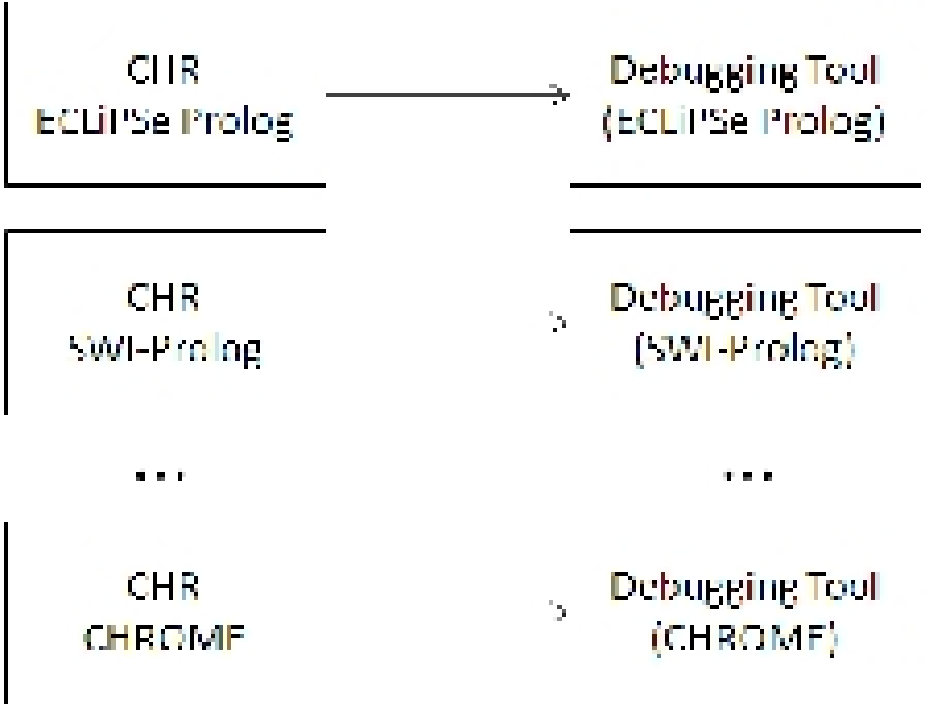
This way each implementation results in a set of one-to-one specialized connections between a solver and its tools. If we want to interchange data between each solver, hooks have to be added into the solver code in order to be able to do it. Furthermore, the types of basic information required by a given debugging tool is not often made explicit and may have to be reverse-engineered. This is a non neglectable part of the cost of porting debugging tool from one constraint programming platform to another.
In order to solve the above-mentioned problem and improve analysis and maintenance of rule-based constraint programs, like CHR∨, there is a need for user-friendly reasoning explanatory facilities that are flexible and portable.
Given this scenario we take advantage of the recent research in trace engineering [16, 14, 15] to propose a generic architecture that produces generic debugging informations for CHR∨ and potential extensions. In that way, any debugging tool changes its focus to generic traces, instead of to be concerned in specific platform implementations.

The Figure 3 illustrates the idea of “generic trace”, which is as independent as possible from a particular CHR platform or specific usages. It shows the structure of a tracing process which can be decomposed into three likely “independent” components: trace extraction, full trace filtering according to some query, and reconstruction of a sub-trace to be used. It shows also the several aspects which must be specified: a semantics for the generic trace (called Observational Semantics), a query language to select the sub-trace of interest to be used, and a semantics to interpret the selected trace (called Interpretative Semantics).
A generic trace needs to be understood independently from the observed process. For this reason it is necessary to be able to give it a semantics as precise as possible. This is the purpose of the Observational Semantics. It will allow for validation tests and studies of some trace properties before and after implementing it. In this report we focus on the observational semantics of traces.
The Fluent Calculus (FC) is a logic-based representation language for knowledge about actions, change, and causality [54]. As an extension of the classical Situation Calculus [43], Fluent Calculus provides a general framework for the development of axiomatic semantics for dynamic domains. It appears to be well suited to describe the Observational Semantics and, though its Flux implementation [53], to be a likely executable specification.
1.4 Connecting all the Pieces
The CHROME project focuses on extending CHR with rule-base encapsulation in software components for reuse by assembly across applications. It has as intention to produce the first domain-independent framework highly reusable debugging tool, supporting a variety of reasoning explanation facilities. The main contribution is to permit any CHR∨ engine to be extensible with components for comprehensive, flexible and efficient reasoning explanation trace generation and user-friendly trace query specification and trace visualization. To achieve this is necessary to integrate design patterns for tracing facilities such as tracer driver with design patterns for Graphical User Interface (GUI) such as Model-View-Controller (MVC) within an overall Model-Driven Architecture (MDA) framework [3]. It will also involve defining a comprehensive trace query language, as well as experiments to empirically evaluate the engineering productivity gains obtained through the use of the tracing components.

In the report we describe the approach illustrated by the Figure 4. It consists first in an observational semantics of the extensible generic trace of CHR which is specified in Fluent Calculus. This semantics is thus mapped into the PIM description of CHROME, leading to a complete PIM of CHROME-REF in UML, the constraint solving and rule based reasoning engine with explanatory traces.
The CHROME-REF environment will be built such an editor as a Eclipse Plugin ††footnotetext: http://www.eclipse.org/ for rapid prototyping deployed with a GUI to interactively submit requests and inspect solution explanations at various levels of details.
The rest of this report is organized in three main sections.
The Section 2 presents a restricted trace meta-theory focused on trace production components and composition. It introduces also the observational semantics of a trace and its representation in the simplified fluent calculus.
The Section 3 presents the observational semantics of CHR∨ in fluent calculus including tracer and extraction schemes.
The Section 4 shows the introduction of the tracer in the PIM of CHROME using the KobrA2 method and resulting in a PIM of CHROME-REF with a very first implementation.
Four annexes give respectively a description of the Observational Semantics of CHR in SFC, the XML scheme of a generic trace of CHR∨, a short example of trace produced by the java compiled CHROME-REF, and the OS of an application.
2 Specifying Tracers
The Trace Meta-Theory (TMT) [15] provides a set of definitions about how to design a trace for a specific domain of observation.
A trace may be interpreted as a sequence of communication actions that may take place between an observer and an observed process. It consists of finite unbounded sequences trace events. There is also the tracer that means the generator of trace. According to [14], the TMT focuses particularly on providing semantics to tracers and the produced traces as independent as possible from those of the processes or from the ways the tracers produce them.
There are two concepts of trace [14] (cf. the Figure 5 and the Section 2.2). The first one is the virtual trace, it represents a sequence of events showing the evolution of a virtual state which contains all that one can or wants to know about the observed process. The second one is called actual trace, it represents the generated trace in the form of some encoding of the current virtual state. Finally, there is the idea of full trace if the parameters chosen to be observed about the process represent the totality of useful knowledge regarding it (explicitly or implicitly).
2.1 Components of Trace Generation and Use
The Figure 6 shows the different components related to a unique trace. We distinguish 5 components, in this order.
- 1.
Observed process
The observed process is assumed more or less abstracted in such a way that his behavior can be described by a virtual trace, that is to say, a sequence of (partial) states. A formal description of the process, if possible, can be considered as a formal semantics, which can be used to describe the actual trace extraction.

Figure 5: Virtual and Actual Trace. - 2.
Extractor
This component is the extraction function of the actual trace from the virtual trace. From a theoretical point of view, we can see it as a specific component, but in practice it corresponds to the tracer whose realization, in the case of a programming language, usually requires modifying the code of the process.
- 3.
Filter
The role of the filter component, or driver [32], is to select a useful sub-trace. This component requires a specific study. It is assumed here that it operates on the actual trace (that produced by the tracer). The fact of making it as a proper component corresponds to the specific approach adopted here, which implies that the extracted actual trace is full. The filtering depends on the specific application, implying that the full trace already contains all the information potentially needed for various uses.
- 4.
Rebuilder
The reconstruction component performs the reverse operation of the extraction, at least for a subpart of the trace, and then reconstructs a sequence of partial virtual states. If the trace is faithful (i.e. no information is lost by the driver) [15], this ensures that the virtual trace reconstruction is possible. In this case also, the separation between two components (rebuilder and analyzer) is essentially theoretical; these two components may be in practice very entangled.
- 5.
Analyzer
The component using a trace may be a trace analyzer or any application.

With these components it may be associated three main specification steps, as illustrated on the Figure 7.

- -
Observational Semantics (OS)
The OS describes formally the observed process (or a family of processes) and the actual trace extraction. This aspect will be studied deeper in the Section 2.2. The intention here is to express the OS using simple fluent calculus.
- -
Querying
Due to the separation in several components, the actual trace may be expressed in any language. We suggest using XML. This allows to use standard querying techniques defined for XML. This aspect will not be developed here, but we chose to express the trace in XML and give in the Appendix B the corresponding XML schema.
- -
Interpretative Semantics (IS)
The interpretation of a trace, i.e. the capacity of reconstructing the sequence of virtual states from an actual trace, is formally described by the Interpretative Semantics. In the TMT no particular application is defined; its objective is just to make sure that the original observed semantics of the process has been fully communicated to the application, independently of what the application does.
2.2 Contiguous Full Traces
We introduce here the two traces which may be associated to a single process equipped with a tracer. We recall here the definitions used in [15].
2.2.1 Virtual Trace
A full virtual trace is defined on a domain of states. Given a finite set of (names) of parameters defined on the domains . The are domains of objects of any kind. They may also have relations (functional or otherwise) between them and they can be infinite in size.
A domain of states is defined on the Cartesian product of the parameter domains: .
Definition 1 (Contiguous Full Virtual Trace)
A contiguous full virtual trace is a sequence of trace events of the form , where:
- •
: is the chrono, specific time of the trace. It is an integer increased by one unit in each successive event. To point a particular value of the chrono, we will talk about moment of the trace.
- •
: an identifier of action characterizing the type of actions undertaken to make the transition from state to state .
- •
: is an element of the state domain. is the current state reached at moment , and the are values of the parameters at moment . is the current full virtual state.
A finite virtual trace over events will be denoted , where is the initial full virtual state and represents the sequence .
The full virtual trace is contiguous insofar as all the moments in the interval are present in the trace .
2.2.2 Actual Trace
The full virtual trace represents what we want or what is possible to observe of a process. It describes the development stages of this process in the form of the evolution of a state which contains the observables. As the current virtual state of a process can be fully represented in this trace, one cannot expect neither to produce it nor to communicate it efficiently. In practice we will perform a kind of “compression” of the information conveyed by the virtual states and their evolution, transmitted or communicable to the process observers, and one shall ensure that these processes are able to “decompress” it. This actually communicated information is the actual trace.
An actual full trace is defined on an actual state domain. Let be a finite set of (names of) attributes defined on domains of attributes . The attributes may have relationships (they are not necessarily independent) and they can be infinite in size.
An actual state domain is defined on the Cartesian product of attributes domains: .
Definition 2 (Contiguous Full Actual Trace)
An actual trace is a sequence of trace events of the form , where:
is the chrono and denotes a finite sequence of attributes values. is the current actual state. The number of attributes of a trace event is bound by . Each state contains at most attributes whose number depends exclusively on the type of action which produced it.
An actual trace with events is denoted , where is the initial virtual state common to both traces and represents the sequence .
2.3 Generic Trace and Composition
We study here the methodology of generic full trace development for a multi-layer based application.
2.3.1 Generic Trace of a Familly of Observed Processes
Consider again the Figure 3 in the introduction. It illustrates the fact that different implementations of CHR can be abstracted by a unique simpler model. This common model is used to specify the unique virtual and actual traces of these implementations. This illustrates the way we will proceed to get a generic trace of CHR: starting from an abstract theoretical, general but sufficiently refined, semantics of CHR which is (almost) the same implemented in all CHR platforms.
2.3.2 Composition of Traces
Now we consider the case of an application written in CHR. It may be for example a particular constraints solver like CLP(FD). In this case there exists already a generic trace called GenTra4CP [12]. This trace is generic for most of the CLP(FD) existing constraints solvers. Therefore a tracer of CLP(FD) solver implemented in CHR should also produce this trace. But we may be interested in refining the trace considering that there are two layers: the layer of the application (CLP(FD)) and the layer of the language in which it is implemented (CHR). The most refined trace will then be the trace in the GenTra4CP format extended with elements of the generic full trace of CHR alone. The generic full trace of CLP(FD) on CHR is an extension of the application trace taking into account details of lower layers.
This is illustrated by the Figure 8 in the case of two layers: an application (like CLP(FD) for example) implemented in CHR. This method can be generalized to applications with several layers of software. The Figure 5 shows in fact at least 4 layers.

In our components based approach it means that we may define separately and independently specific generic full traces for each layer, and, so in this case for the application (APL) and the under-layer of CHR. The generic full trace APL on CHR is a kind of composition of traces and will be obtained by some merging of both generic full traces into a unique one. The result may not exactly be a union of all actions, parameters and attributes, but it is not our purpose here to study more deeply this aspect. For more details see [15].
2.4 Observational Semantics
The Observational Semantics (OS) is a description of a possibly unbounded data flow without explicit reference to the operational semantics of the process which produced it [16]. The OS may be considered as a abstract model of process, in the case of a single observed process or it can be an abstraction of the semantics to several processes. It is defined as a Labelled Transition Systems (LTS) [25].
2.4.1 Representation of the Observational Semantics
The Observational Semantics has two parts: a state transition function and a trace extraction function.
The first part is a formal model on the way successive events of the virtual trace are related.
It is a virtual trace semantics in the sense that, given a full virtual trace
, it explains the sequence of events by a transition function33
3
It is fact a relation since the transitions may be nondeterministic. recursively applied from an initial virtual state.
The second part, the function of extraction, produces what is actually “broadcasted” outside from the observed process. This function has as arguments the current state and the type of action, and produces the attributes of the actual trace.
Definition 3 (Observational Semantics (OS))
An Observational Semantics is defined by the tuple , where
- •
is a virtual state domain, where each state is described by a set of parameters.
- •
is a finite set of action types, set of identifiers used as labels for transitions.
- •
is a actual state domain, where each state is described by a set of attributes.
- •
is the local extraction function of the actual state , performed by transition of action type issued from state , x , which satisfies by definition: (, set of actual states). More precisely, the set of attributes of the event of the actual trace is derived from the current state at moment of the virtual trace and the transition labelled by the action type , i.e.
- •
state transition function x , i.e.
- •
, set of initial states.
The OS may be represented by “rules”, one for each action, describing the transition and the actual trace event extraction corresponding to the action. A rule has 4 items.
- •
AType: an action identifier
- •
ACond: { some auxiliary computations on the current virtual state and condition for executing the action corresponding to the transition: a first-order logic formula using predicates on the parameters }
- •
VSEffect: { the effect of the action on the current state , resulting in a new state , and some auxiliary computations relative to the attributes of the trace event }
- •
Etrace: { the attributes of the trace event produced by the action : , new extracted actual trace event }
Example 2.1: the Fibonacci Function
Idealized (biologically unrealistic) rabbit population.
The OS , describes the deterministic transition function .
: (positive integers list), is the complete evolution of the population from moment until moment :
: {} (monthly growing)
: , is the population at moment ().
: . There is one rule only to describe .
: (respectively before last and last elements of the list s, denote lists concatenation). The new virtual state is the previous state to which the sum of the two last elements is appended.
: .
AType:
ACond: { }
VSEffect: { }
Etrace: {}
Traces:
2.4.2 Simple Fluent Calculus
The Fluent Calculus (FC) is a logic-based representation language for knowledge about actions, change, and causality [54]. As an extension of the classical Situation Calculus [43], Fluent Calculus provides a general framework for the development of axiomatic semantics for dynamic domains.
The simple fluent calculus (SFC) has the following appealing qualities:
- -
Simplification of the description, since the notions of virtual state and actual trace are “naturally” embedded in the fluent calculus (the situation corresponding to a state can be viewed as a representation of the actual trace).
- -
Reasoning on transitions may be simpler, as it supports handling partial virtual states (with appropriate axiomatisation). Formal proofs become simpler in the SFC (less deductions, at least for “direct closed” effects, see [54, 51]). It follows that properties like “faithfulness” [16] should be easier to prove formally. The Symmetry of “state axioms” allows forward and backward reasoning. With the simplicity of the representation of state changes, this should make such proofs simpler.
- -
The description in SFC makes such specification potentially executable in Flux. There is some limits to the executability, related to the partial axiomatisation of the observational semantics and executability of formal specification in general. However such framework may facilitate some simulations.
The Fluent Calculus is a sorted logic language with four standard sorts: FLUENT, STATE, ACTION, and SIT (which stands for situation). A fluent describes a single state property that may change by the means of the actions of some agent. A state is a collection of fluents. Adopted from Situation Calculus, the standard sort SIT describes sequences of actions.
The pre-defined constant stands for the empty state. Each term of sort FLUENT is also an (atomic) STATE, and the function , written in infix notation, represents the composition of two states. The following abbreviation is used to express that fluent holds in state :
| (1) |
The behavior of function “” is governed by the foundational axioms of Fluent Calculus, which essentially characterize states as sets of fluents.
| (2) |
| (3) |
| (4) |
| (5) |
| (6) |
States can be updated by adding and/or removing one or more fluents. Addition of a sub-state to a state is simply expressed as , and removal is defined by
| (7) |
The standard predicate in Fluent Calculus is used to axiomatize the conditions under which an action is possible in a state, i.e., the situations in which the pre-condition of this actions is satisfied.
The pre-defined constant is the initial (i.e., before the execution of any action) situation. The function denotes the addition of an action to a situation. The standard function is used to denote the state, i.e., the fluents that hold in a situation, after a sequence of actions. This allows to extend macro Holds and predicate to SITUATION arguments as follows.
| (8) |
| (9) |
In a Fluent Calculus Axiomatization, beyond the definition of the domain sorts, functions and predicates, we can define a set of axioms that must follow three pre-defined axiom schemas: the precondition axioms, the state update axioms and the state constraint axioms.
Definition 4 (Pure State Formula)
A Pure State Formula is a First Order formula
- •
There is only one free state variable
- •
It is composed of atomic formulas in the form:
, where is of the sort FLUENT
atoms which do not use any reserved predicate of Fluent Calculus
Definition 5 (Precondition Axiom)
A precondition axiom follows the schema: , where is a Pure State Formula.
This kind of axiom states that the execution of the action with the parameters is possible in the state if and only if is true.
Definition 6 (State Update Axiom)
A state update axiom follows the schema:
where
where
and are partial states.
2.4.3 Observational Semantics in Simple Fluent Calculus
A virtual state of the observed process corresponds to a state in SFC described by a set of fluents (this correspondence must be explicitly specified).
Each type of action in the OS is an action name in the SFC. A particular action is denoted in the following.
Actual states are elements of the Cartesian product of attribute domains (this domain must be explicitly specified).
Transition and extraction function (or relation) are described using both fundamental following schemes (fundamental axioms of the Fluent calculus)
- 1.
Pre-Condition Axioms:
- 2.
State Update Axioms:
where is an actual trace event associated with the transition, and derived from the current state (using local variables too).
There are as many pre-conditions and state update axioms as there are action types in the OS. may be a disjunction. It defines the new virtual state and the corresponding extracted actual trace event attributes .
Nota: a situation contains the sequence of actions in the OS executed to reach the current virtual state , and also the sequence of extracted actual trace events such that .
An actual trace is the sequence of , with chrono, found in the situation
It may be computed according to the following axioms:
Example 2.2: OS for Fibonacci
The virtual state contains only one fluent of type , and there is only one type of action . The actual state contains just 2 attributes, respectively of type and . A vector is represented by a sequence (Prolog list syntax).
2.5 Trace Query and Analysis Tools
Trace query and analysis tools are considered here as separate components, as illustrated in the Figure 6. Although they are part of the CHROME-REF project, they are not studied more deeply here. Instead, we propose a first repesentation of the actual CHR trace using XML. The XML schema is given in the Appendix B, and an example of produced trace in the XML format in the Appendix C.
3 Tracing Rule-Based Constraint Programming
Constraint Handling Rules emerges in the context of Constraint Logic Programming (CLP) as a language for describing Constraint Solvers. In CLP, a problem is stated as a set of constraints, a set of predicates and a set of logical rules. Problems in CLP are generally solved by the interaction of a logical inference engine and constraint solving components. The logical rules (written in a host language) are interpreted by the logical inference engine and the constraint solving tasks are delegated to the constraint solvers.
3.1 CHR by Example
The following rule base handles the less-than-or-equal problem:
This CHR program specifies how simplifies and propagates as a constraint. The rules implement reflexivity, antisymmetry, idempotence and transitivity in a straightforward way. CHR states that simplifies to , provided it is the case that . This test forms the (optional) guard of a rule, a precondition on the applicability of the rule. Hence, whenever we see a constraint of the form we can simplify it to true.
The rule means that if we find as well as in the constraint store, we can replace it by the logically equivalent . Note the different use of in the two rules: in the rule the equality is a precondition (test) on the rule, while in the rule it is enforced when the rule fires. (The reflexivity rule could also have been written as )
The rules and are simplification CHR. In such rules, the constraint found are removed when the rule applies and fires. The rule is a simpagation CHR, only the constraint in the right part of the head will be removed. The rule says that if we find and another in the constraint store, we can remove one.
Finally, the rule states that the conjunction implies . Operationally, we add as (redundant) constraint. without removing the constraints . This kind of CHR is called propagation CHR.
The CHR rules are interpreted by a CHR inference engine by rewriting the initial set of constraints by the iterative application of the rules. Its extension with disjunctive bodies, CHR∨ boosts its expressiveness power, turning it into a general programming language (with no need of an host language).
3.2 Observational Semantics of CHR
The observational semantics of a tracer is based on a simplified abstract semantics of the observed process. In the case of CHR∨, we suggest to use an adaptation of the refined theoretical semantics of CHR as presented in [17]. To start with, we show how to build an observational semantics for CHR based on the theoretical operational semantics [22]. The description of in SFC is borrowed from [9].
3.2.1 Theoretical Operational Semantics of CHR
We define as the constraint theory which defines the semantic of the built-in constraints and thus models the internal solver which is in charge of handling them. We assume it supports at least the equality built-in. We use to indicate the first () and the remaining () terms in a list, for sequence concatenation and for empty sequences.
We use the notation for both bags and sets. Bags are sets which allow repeats. We use for set union and for bag union, and {} to represent both the empty bag and the empty set. The identified constraints have the form , where c is a user-defined constraint and i a natural number. They differentiate among copies of the same constraint in a bag. We also assume the functions and .
An execution state is a tuple , where is the Goal, a bag of constraints to be executed; is the UDCS (User Defined Constraint Store), a bag of identified user defined constraints; is the BICS (Built-In Constraint Store), a conjunction of constraints; is the Propagation History, a set of sequences, each recording the identities of the user-defined constraints which fired a rule; is the next free natural used to number an identified constraint.
The initial state is represented by the tuple . The transitions are applied non-deterministically until no transition is applicable or the current built-in constraint store is inconsistent. These transitions are defined as follows:
Solve where is built-in
Introduce where is user-defined constraint
Apply where exists a rule
and a matching substitution ,
such that and and the sequence
and
Example 3.1 The following is a (terminating) derivation under for the query executed on the leq program in Example 3.1. For brevity, have been removed from each tuple.
| (1) | |||
| (2) | |||
| (3) | |||
| (transitivity r4 ) | (4) | ||
| (5) | |||
| (6) | |||
| (antisymmetry r2 ) | (7) | ||
| (antisymmetry r2 ) | (8) |
No more transition rules are possible, so this is the final state.
3.2.2 Theoretical Operational Semantics of CHR in SFC
The following is the description of the theoretical operational semantics in terms of the sorts, relations, functions and axioms of the simple fluent calculus.
- (a)
Domain Sorts
- -
, natural numbers;
- -
, the sort of CHR rules and the sort of the rule identifiers;
- -
, the sort of constraints, with the following subsorts: (the built-in constraints), with the subsort (constraints in the form ), and (the user-defined constraints), with the following subsort: (constraints in the form ). In short:
and
;
- -
, the elements of the Propagation History, tuples of a sequence of natural numbers and a rule;
For each defined sort , three new sorts: , and containing the sequences, the sets and the bags of elements of . We use [] for the empty sequence and {} for the empty set and the empty bag.
- -
, the subsort of containing only the actions in the CHR semantics.
- -
- (b)
Predicates
- -
, holds iff is the initial query;
- -
, holds iff the of the state is consistent (i.e., if it does not entail false).
- -
holds iff (i) and are in the of and (ii) the set of matching equations e is such that and ;
- -
, holds if .
- -
- (c)
Functions
- -
, defines the syntactic sugar for defining identified constraints in the form ;
- -
,
makes a rule from its components. We define the syntactic sugar for rules as ;
- -
, where ;
- -
, where
- -
The usual set, sequence and bag operations: for element, for set union, for bag union, for sequence concatenation, for sequence head and tail (Ex: ) and for set subtraction.
- -
- (d)
Fluents
- -
, holds iff is the current goal;
- -
, holds iff is the current UDCS;
- -
, holds iff is in the current BICS;
- -
, holds iff is in the current Propagation History;
- -
, holds iff is the next natural number to be used to identify a identified constraint.
- -
- (e)
Actions
- -
, executes the transition with the built-in constraint ;
- -
, executes the Introduce transition with the user-defined constraint ;
- -
,
executes the Apply transition matching the constraints and in the with the kept and removed heads of .
- -
- (f)
Axioms
- -
,
The Initial State Axiom states that in the initial state, the goal contains the constraints in the query, the user defined constraint store is empty and the next ID for identified constraints is 1;
Solve
- -
The Solve Precondition Axiom states that the only precondition for the action on the built-in constraint is that this constraint should be in the goal.
- -
The Solve State Update Axiom states that the result of the action over the constraint is that this constraint is removed from goal and added to list in current state;
Introduce
- -
- -
Apply
- -
- -
- -
3.2.3 Observational Semantics of CHR based on
The following is the description of the observational semantics of CHR using the simple fluent calculus with modified axioms of the Section 2.4.3. Sorts, Predicates, Functions and Fluents are the same as in the previous section; there is on additional item for the attributes.
The actions are now constants and we make explicit 4 actions:
.
-
(e) Actions
- -
, executes the top-level initial transition (starting the resolution) with some query in the current state ( stands for other attributes list in the associated trace event);
- -
, executes the transition with the built-in constraint ;
- -
, executes the Introduce transition with the user-defined constraint ;
- -
,
executes the Apply transition with rule matching the constraints in the with the kept and removed heads;
- -
, if no is possible.
There are also 5 attributes in the actual trace: .
- -
-
(f) Attributes
- -
, is the set of constraints in the current Goal;
- -
, is the set of constraints in the current User Defined Constraints Store;
- -
, is the set of constraints in the current Built-In Constraints Store ;
- -
, is the new propagation history index (incremented by );
- -
, is the rule applied to reach this state.
Apply
We just comment the adaptation of one rule, the full description is in Appendix A.
- -
-
(g) Axioms of the Observational Semantics
- -
- -
[apply, ]
- -
The observational semantics of CHR∨ can be formalized similarly with 11 actions (hence 11 different kinds of trace events),
,
3.3 Towards Full Generic Trace of CHR∨
As suggested in the Section 2.3.2, a full trace will be progressively obtained by composing several layers of traces and several potential applications in such a way that as many as possible of potential uses can be satisfied by such a trace. The Figure 5 suggests 4 levels of refinements corresponding to 4 layers of implementations, i.e. from bottom to top: environment of execution (Windows/Linux/Mac…), implementation language (most of CHR are implemented in Prolog), CHR, and application written in CHR. There may be other lower levels, like WAM abstract machine implemented in Java for the Prolog level, etc… Even if each layer has its own level of abstraction and most of the CHR users don’t care about lower software layers, it may be interesting to keep some trace of them in the “full” trace.
If we consider the point of view of debugging some application written in CHR, here are some information which could be usefully found in a trace used by a debugging tool.
- •
Execution environment: activation of system commands during interactions
- •
Implementation languages (there may be several layers): specific local error messages, activated layer, …
- •
CHR: name of used rules
We mean here that, at some point, it may be useful to find in the trace of the application some information regarding different layers of implementation in order a debugging tool to be able to “understand” some bugs.
Let us consider an example of application. In the Annex D we give the observational semantics in SFC of a simple application of [53]. This OS specifies possible traces of actions performed by robots (here there is only one). We may assume that this small world is programmed in CHR and therefore the trace of the whole system is a kind of combination of both traces: the one of the robot and the trace corresponding to the CHR program execution. The resulting full trace corresponds to the trace composition described in the Section 2.3.2 (comprehensively treated in [15]).
If one wants just to follow what the robots are doing, then the sub-trace consisting of the trace events regarding the robot’s actions is sufficiently relevant. But, at least at the stage of debugging, some dysfunction observed in the robot’s trace (for example crossing a closed door) can be understood only by looking at a more complete trace which includes events related to the CHR layer behaviour.
Finally there is one more level, which corresponds to the specificity and versatility of CHR: the many extensions and applications which are embedded in CHR with CHR as implementation language, quoted as the “CHR world” in the introduction. Here are some of them [22]: Boolean algebra for circuit analysis, resolution of linear polinomial equations - CLP()44 4 CLP stands for Constraint Logic Programming.- with application in finances and non linear equations, finite domain solvers - CLP(FD) - with applications in puzzles, scheduling and optimisation, but many others as quoted at the beginning of the report.
A full CHR∨ trace should probably include traces related to several extensions like CLR() where stands for some constraint domain, and CHRV;naf for example. This is possible, but there is still a need to specify an observational semantics for several of these extensions.
4 Towards CHROME-REF
This section details the architecture of CHROME-REF, the extensible implementation of a generic tracer for Constraint Solving and Rule-Based Reasoning. Each component of the CHROME-REF is described in terms of UML2.1 according the KobrA2 methodology [4, 5]. We first give a brief overview of CHROME.
4.1 CHROME
CHROME stands for Constraint Handling Rule Online Model-driven Engine, is a model-driven, component-based, scalable, online, Java-hosted CHR∨ engine to lay at the bottom of the framework as the most widely reused automated reasoning component. The idea of CHROME is also to demonstrate how a standard set of languages and processes prescribed by MDA can be used to design concrete artefacts, such as: a versatile inference engine for CHR∨ and its compiler component that generates from a CHR∨ base the source code of Java classes.
4.1.1 Goals and Design Principles
The main goal of CHROME if to take CHR engines a step beyond, by designing a new CHR∨ engine and a corresponding compiler using a component-based model-driven approach. CHROME is a CHR∨ engine with an efficient and complete search algorithm (e.g. the conflict-directed backjumping algorithm), the first versatile rule-based engine, integrating production rules, rewrite rules, its built-in belief revision mechanism (reused for handling disjunctions) and CLP rules to run on top of a mainstream Object Oriented (OO) platform (Java). Because it is a rule-based engine following a component-based model-driven approach, it allows easy port to other OO platforms such as Python, JSP, C++ and others. Finally the compiler is the first that uses a model transformation pipeline to transform from a source relational-declarative language into a OO imperative paradigm language.
The CHROME architecture is divided into two main sub-components (see the Figure 9):
- i)
The ATL-pipeline compiler (CHR Compiler component) that takes as input a relational declarative CHR∨ base and produces an efficient constraint handling imperative object-oriented component assembly.
- ii)
The CHROME run-time engine (shown in the Figure 9 as the QueryProcessor component) that provides the services and data structures necessary to execute a CHR∨ base given a particular query (collection of constraints).

The Figure 10 shows the complete MOF metamodel of CHR∨. At this abstract syntax level all CHR∨ rules are generalized as simpagation rules. The meta-associations keep and del from the CHR∨ meta-class to the Constraint meta-class respectively represent the propagated and simplified heads of the rule. The heads must be instances of RDCs (Rule Defined Constraints). A guard of a rule must be a collection of BICs (BuiltIn Constraints). Both RDCs and BICs are specializations of Constraint meta-class.

The body of a CHR∨ rule is a collection of alternative conjunctions. Conjunctions are composed by both RDC or BIC, e.g. a collection of instances of meta-class Constraint. The original CHR∨ base has a special RDC (OR) to indicate disjunctions in the body. The collection of all rules of a CHR program is a CHR Base.
Each constraint is composed by a constraint symbol and a collection of zero or more arguments, e.g. a collection of terms (meta-class Term). A Term further specializes into: functional terms, non-functional terms, ground terms and non-ground terms. A Constant is both a non-functional term and a ground term and a Variable is a non-ground term and a non-functional term. Finally a functional term is further composed by a Function Symbol and a collection of zero or more arguments, which are in turn recursively defined as instances of meta-class Term. The constraint domain meta-class aggregates all term symbols allowed.
The metamodel displays also the internal structures of the engine, namely: the constraint store and the constraint queue. The first stores the constraints added by firing rules, the second is a processing queue that tracks which is the next constraint to be processed.
4.1.2 Strengths and Limitations
CHROME is the first Java CHR∨ engine: none of the related CHR Java engines allow disjunctive rules. Compilation in Java makes it easier to reuse and deploy full CHR∨ bases in applications in need of automated reasoning services. It is one of the largest case study to date to integrate MDE technology with model transformations (4358 ATL lines) and components. It however suffers some limitations, as it provides only three built-in constraints: the syntactical equality, true and false, and it has no visual tracing IDE. This makes practical applications still too cumbersome to implement, being tracing a fundamental part of large automated reasoning development.
4.2 CHROME-REF Components
The Figure 11 shows a object-oriented representation of the observational semantics of CHR∨ as described in the Section 3.2.1. It contains five sort of extracted trace events (): an initial state (), user-defined contraint store introduced (), built-in introduced (), rule applied () and rule failed ().

The top-level CHROME-REF component encapsulates all sub-components that compose the CHROME environment. The Figure 12 shows the main component and its three sub-components as defined in what follows. They provide methods to compile a rule base, to solve a query (displaying one or more solutions for such query), to adapt a solution when a given set of justified constraints is deleted and to clear the constraint store for processing a new query.

The Driver component is a intermediator between CHROME and Analyzer, its function is to manager the communication of trace event sent by the engine and filter the requested information to the analyzer. Finally, the Analyzer component, in our case, is a debugging tool for CHR.
The next sub-sections describe each component.
4.2.1 Extraction
The Figure 13 shows the CHROME component with a new component called TraceExtraction, which implements the generic CHR trace as described in the Section 3.2.3.

We have added two improvements to the CHROME to integrate with our proposal: a new componente called Trace Extraction that receives as input some parameters () and produces the trace events (); and, we included new rules into the CHROME compiler to send the previous parameters to the Trace Extraction during the execution of a CHR program.
The following OCL rules explain how a trace event will be produced from received parameters:
4.2.2 Driver
The Trace Driver component is an intermediator between a process and an analyzer. It component has the following functions (Figure 14):
- •
to decide whether the underlying process (in our case CHROME) will send trace events step by step or all at once. This information is represented by means of the flag ;
- •
to register an analyzer that will watch the trace events from the underlying process;
- •
to notify all connected analyzers soon after a trace event to be produced;
- •
to ask for a new trace event (only if the flag is true); and,
- •
to filter a trace event by means of a trace query sent from a analyzer.

The following OCL rules describe the post-condition of each method:
As said before, the Trace Driver component is a intermediator that receives trace events from a process and sends it to the analyzer. The Figure 15 shows the relationships between these components.

A trace driver is connected to an observed process which sends the trace events, and it has a list of analyzers to which to the trace events. Each analyzer is associated to a query, which says which information the driver will send to the analyzer.
4.2.3 Analyzer
The trace analyzer specifies to the driver which events are needed by means of queries. The requests that an analyzer can send to the tracer driver are of three kind. Firstly, the analyzer can ask for additional data about the current event. Secondly, the analyzer can modify the query to be checked by the driver. Thirdly, the analyzer can notify the driver to pause, continue or end the process execution.
In this project, in order to exemplify the whole proposed framework, we have created two simple views to show a pretty-printing of a CHR execution. The Figure 16 presents these two kind of analyzers: the shows the evolution of the CHR parameters (Goal, Constraint Store, Built-ins, etc), defined in the generic trace; and the is just to focus in a specific rule when this rule is triggered.
We illustrate these views with an execution of the LEQ example.
with the query:

Finally, we get the XML instance produced by CHROME for this example (see complete trace with all attributes in the Appendix C).
At this stage of the implementation, such views are principally helpful to help to develop the generic trace.
5 Conclusion
In this report we have presented an ongoing work as a roadmap towards CHROME-REF, and we have defined the methods and tools to reach this goal. They consists of a formal specification (called observational semantics - OS) of a generic tracer for CHR∨ using an adaptation of the simple fluent calculus (SFC) which we have presented, and its implementation, over and inside CHROME, using the KobrA2 method, and resulting in a PIM of CHROME-REF.
We have tested the approach with a small trace pretty printing GUI. We also indicated how to work on extensions of the very first trace we presented (using the simple semantics of CHR), before including other actions and attributes inspired by more refined semantics of CHR∨ and various CHR domains extensions.
Several other issues however remain to be explored.
First the use of the SFC to describe the observational semantics of tracers. As quoted in the report, we may expect several advantages of its use: facilitation of trace extension specification, or refinement, by merging observational semantics of several CHR extensions or sublayers, and facilitation of verification of formal properties of the trace. We did not reach the point to be in condition to simulate production of traces trying to execute this OS using Flux. Such execution would require some implementation of complex functions or predicates. Since the OS may be a smooth abstraction of a family of solvers, it is in principle possible to develop some simulation producing supersets of possible traces. This can be useful to analyse some properties of the traces to improve their design. However it will become worth and more interesting when a more refined full trace will be ready.
Another point which remains unsolved is the way to relate the observational semantics of the tracer and the design of the CHROME-REF PIM. Both are forms of partial formal specification. The OS because it is an abstraction of the semantics of the observed process - hence a partial specification-, the later because it is a partially formal specification. Even if it is clear that the description of the tracer in SFC is a clear requirement which serves as guideline to design this PIM, there is no way to guarantee a formal correspondence.
One proposed approach is to map the logical model of SFC used here into an Object-Oriented (OO) model (OOSFC), and to limit the “implementation step” to a merging of PIMs. This way to proceed is illustrated on the Figure 17. This approach aims at reducing the complexity of mapping between the two different descriptions, by introducing a intermediary step denoted CHR-OSOOSFC.
We have started to specify the OS in OOSFC [39], but this question is still open whether this step is really helping, or whether the construction of the tracer part of the CHROME-REF PIM in UML is better achieved just using the SFC specification of the OS. It could be also interesting to compare several approaches of extending existing codes, like pluging aspects in the CHROME java code. In any cases the question of the relationships with the specification is still worth posing.
Finally a third unsolved point concerns the validation of the implementation. Considering the design and implementation used method, there is no way to make formal proof of adequation between the specification and the implementation, but this point need more study. At this stage, we are limited to perform tests. The Figure 18 illustrates this point.


- •
Semi-formal proof: It is to show that CHR-OSFC is equivalent to the CHROME-REFUML. But, as UML is a semi-formal language [33], so that, UML is not stricly formal in sense of a purely syntactic derivation using a very precise and circumscribed formal set of rules of inference, no formal proof can be performed.
- •
Test-based validation: Let CHR-OSFC with its equivalent implementation CHR-OSFlux in Flux, and CHROME-REFUML with its equivalent implementation in Java CHROME-REFJava, the method consists of comparing the produced traces to check whether they are equivalent.
There is still a long way to get a full generic trace for CHR. Indeed, as quoted in the Section 3.3, such goal implies the existence of generic traces for several CHR extensions. Since we already have some (for finite domain solvers, or for Prolog under-layer for example), we are far to cover all existing extensions of CHR quoted at the beginning of this paper. But the composition of traces and the method of implementing tracer presented here give a possible road towards a full generic trace for CHR∨ and many of its extensions.
References
- [1] Abdennadher, S. Rule Based Constraint Programming: Theory and Practice. Habilitation, Institut fur Informatik, Ludwig-Maximilians-Universitat Munchen (2001).
- [2] Aggoun, A. ECLiPSe User Manual. Release 5.3.
- [3] Atkinson, C., Bayer, J., and Bunse, C. Component-based product line engineering with UML. Addison-Wesley Professional, 2002.
- [4] Atkinson, C., Bayer, J., and Muthig, D. Component-based product line development: The KobrA approach. In Software product lines: experience and research directions: proceedings of the First Software Product Lines Conference (SPLC1), August 28-31, 2000, Denver, Colorado (2000), Kluwer Academic Publishers, p. 289.
- [5] Atkinson, C., Robin, J., and Stoll. Kobra2 Technical Report.
- [6] Banker, R., Davis, G., and Slaughter, S. Software development practices, software complexity, and software maintenance performance: A field study. Management Science (1998), 433–450.
- [7] Boehm, B. A spiral model of software development and enhancement. Software Engineering: Barry W. Boehm’s Lifetime Contributions to Software Development, Management, and Research 21, 5 (2007), 345.
- [8] Christiansen, H. Prioritized abduction with CHR. In The 5th Workshop on Constraint Handling Rules (2008), p. 159.
- [9] da Silva, M. A. A. CHORD: Constraint Handling Object-Oriented Rules with Disjunctions. Universidade Federal de Pernambuco. CIn. Ciência da Computação, 2009.
- [10] da Silva, M. A. A., Fages, F., and Robin, J. Default Reasoning in CHR∨. In Proceedings of the 5th Workshop on Constraint Handling Rules (CHR’08) (Hagenberg, Austria, Aug. 2008).
- [11] de Oliveira, C. M. C2HR∨: Component and Rule-Based Constraint Programming and Knowledge Representation, July 2008. Intership final report.
- [12] Deransart & al, P. Outils d’Analyse Dynamique pour la Programmation Par Contraintes (OADymPPaC). Tech. rep., Inria Rocquencourt, École des Mines de Nantes, INSA de Rennes, Université d’Orléans, Cosytec and ILOG, May 2004. Projet RNTL. http://contraintes.inria.fr/OADymPPaC.
- [13] Deransart, P. On using Tracer Driver for External Dynamic Process Observation. Arxiv preprint cs.PL/0701106 (2007).
- [14] Deransart, P. Semantical View of Tracers and their Traces, and Applications. working Draft (2008). http://hal.inria.fr/.
- [15] Deransart, P. Conception de Trace et Applications (vers une méta-théorie des traces), decembre 2009. Working document http://hal.inria.fr/.
- [16] Deransart, P., Ducassé, M., and Ferrand, G. Observational semantics of the Prolog Resolution Box Model. Arxiv preprint arXiv:0711.4071 (2007).
- [17] Duck, G., Stuckey, P., de la Banda, M., and Holzbaur, C. The refined operational semantics of Constraint Handling Rules. Lecture notes in computer science (2004), 90–104.
- [18] Epsilon. The Epsilon Book. http://www.eclipse.org/gmt/epsilon/doc/book/, 2009.
- [19] Eriksson, H. UML 2 toolkit. Wiley, 2004.
- [20] Fages, F., de Oliveira Rodrigues, C. M., and Martinez, T. Modular CHR with ask and tell. In Proceedings of the fifth Constraint Handling Rules Workshop CHR’08 (2008), T. Frühwirth and T. Schrijvers, Eds.
- [21] France, R., and Rumpe, B. Model-driven development of complex software: A research roadmap. In International Conference on Software Engineering (2007), IEEE Computer Society Washington, DC, USA, pp. 37–54.
- [22] Fruhwirth, T., and Abdennadher, S. Essentials of constraint programming. Springer-Verlag New York Inc, 2003.
- [23] GADOMSKI, A. Global TOGA Meta-Theory. 1997-2007 [cit. 2007-12-12]. Dostupnỳz 2 (1997). http://erg4146.casaccia.enea.it/wwwerg26701/Gad-toga.htm.
- [24] Gamma, E., Helm, R., Johnson, R., and Vlissides, J. Design patterns: elements of reusable object-oriented software. 1995.
- [25] Gilmore, S. Trends in functional programming. Intellect L & DEFAE, 2005.
- [26] Heineman, G., and Councill, W. Component-based software engineering: putting the pieces together. Addison-Wesley Longman Publishing Co., Inc. Boston, MA, USA, 2001.
- [27] Henglein, F., and Tofte, M. An introduction to operational semantics of programming languages. Datalogi 2.1 kursusbog 1 (1993), 7–109.
- [28] Kent, S. Model driven engineering. Lecture notes in computer science (2002), 286–298.
- [29] Kolovos, D., Paige, R., and Polack, F. The epsilon object language (eol). Lecture Notes in Computer Science 4066 (2006), 128.
- [30] Korel, B., and Rilling, J. Application of dynamic slicing in program debugging. Automated and Algorithmic Debugging (1997), 43–58.
- [31] Langevine, L., Deransart, P., and Ducasse, M. A generic trace schema for the portability of cp(fd) debugging tools. Lecture notes in computer science (2004), 171–195.
- [32] Langevine, L., and Ducassé, M. A Tracer Driver for Hybrid Execution Analyses. In Proceedings of the 6th Automated Debugging Symposium (Sept. 2005), A. Press, Ed.
- [33] Latella, D., Majzik, I., Massink, M., et al. Towards a formal operational semantics of UML statechart diagrams. In IFIP TC6/WG6, vol. 1, pp. 331–347.
- [34] Mazurkiewicz, A. Trace theory. In Advances in Petri nets 1986, part II on Petri nets: applications and relationships to other models of concurrency table of contents (1987), Springer-Verlag New York, Inc. New York, NY, USA, pp. 279–324.
- [35] Mellor, S., Scott, K., Uhl, A., and Weise, D. Model-driven architecture. Lecture Notes in Computer Science (2002), 290–297.
- [36] Miller, J., Mukerji, J., et al. MDA Guide Version 1.0. 1. Object Management Group 234 (2003).
- [37] Møller, A., and Schwartzbach, M. The design space of type checkers for XML transformation languages. Springer.
- [38] Oliveira, R. F. A Component Based Approach to Specify and Implement Generic Traces in CHROME. Internship final report, INRIA Paris-Rocquencourt, Dec. 2009.
- [39] Oliveira, R. F. Theoria de Rastros em OOFC. Relatorio de Graduação, UFPe, Mar. 2009.
- [40] OMG. Object Management Group, August 2009. http://www.omg.org/.
- [41] Pilone, D., and Pitman, N. UML 2.0 in a Nutshell. O’Reilly, 2005.
- [42] Proctor, M., Neale, M., Lin, P., and Frandsen, M. Drools documentation.
- [43] Reiter, R. The frame problem in the situation calculus: A simple solution (sometimes) and a completeness result for goal regression. Artificial intelligence and mathematical theory of computation: papers in honor of John McCarthy (1991), 359–380.
- [44] Reyna, V., and Brainerd, C. Fuzzy-trace theory: An interim synthesis. Learning and Individual Differences 7, 1 (1995), 1–75.
- [45] Richer, M. An evaluation of expert system development tools. AI tools and techniques (1989), 67.
- [46] Richters, M., and Gogolla, M. A metamodel for OCL. In The Unified Modeling Language: UML’99: Beyond the Standard: Second International Workshop, Fort Collins, CO, October 28-30, 1999: Proceedings (1999), Springer Verlag, p. 156.
- [47] Robin, J., and Vitorino, J. ORCAS: Towards a CHR-based model-driven framework of reusable reasoning components. See Fink et al.(2006) (2006), 192–199.
- [48] Schneidewind, N. The state of software maintenance. IEEE Transactions on Software Engineering (1987), 303–310.
- [49] Schrijvers, T., and Demoen, B. The KU Leuven CHR system: Implementation and application. In First workshop on constraint handling rules: selected contributions (2004), vol. 2004, Citeseer, p. 01.
- [50] Schrijvers, T., Demoen, B., Duck, G., Stuckey, P., and Fruhwirth, T. Automatic implication checking for CHR constraints. Electronic Notes in Theoretical Computer Science 147, 1 (2006), 93–111.
- [51] Shanahan, M. The Frame Problem. In The Macmillan Encyclopedia of Cognitive Science (Dec. 2003), N. L., Ed., Macmillan, pp. 144–150.
- [52] Sneyrs, J., VAN WEERT, P., T., S., and L., D. K. As Time Goes By: Constraint Handling Rules. A Survey of CHR Research from 1998 to 2007. Learning and Individual Differences (2003), 1–49.
- [53] Thielscher, M. Introduction to the fluent calculus. Electronic Transactions on Artificial Intelligence 2 (1998), 179–192.
- [54] Thielscher, M. From situation calculus to fluent calculus: State update axioms as a solution to the inferential frame problem. Artificial Intelligence 111, 1 (1999), 277–299.
- [55] Van Weert, P. Efficient Lazy Evaluation of Rule-Based Programs.
- [56] Vitorino, J. Model-Driven Engineering a Versatile, Extensible, Scalable Rule Engine through Component Assembly and Model Transformations. Universidade Federal de Pernambuco. CIn. Ciência da Computacão, 2009.
- [57] Warmer, J., and Kleppe, A. The object constraint language: precise modeling with UML. Addison-Wesley Longman Publishing Co., Inc. Boston, MA, USA, 1998.
- [58] Wielemaker, J. SWI-Prolog 5.6 Reference Manual. Department of Social Science Informatics, University of Amsterdam, Amsterdam, Marz (2006).
Appendix A Appendix - Observational Semantics of CHR
The following is the description of the observational semantics of CHR based on its theoretical operational semantics and the simple fluent calculus with modified axioms of the Section 2.4.3.
- (a)
Domain Sorts
- -
, natural numbers;
- -
, the sort of CHR rules and the sort of the rule identifiers;
- -
, the sort of constraints, with the following subsorts: (the built-in constraints), with the subsort (constraints in the form ), and (the user-defined constraints), with the following subsort: (constraints in the form ). In short:
and
;
- -
, the elements of the Propagation History, tuples of a sequence of natural numbers and a rule. For each defined sort , three new sorts: , and containing the sequences, the sets and the bags of elements of . We use [] for the empty sequence and {} for the empty set and the empty bag.
- -
, the subsort of containing only the actions in the CHR semantics.
- -
- (b)
Predicates
- -
, holds iff is the initial query;
- -
, holds iff the of the state is consistent (i.e., if it does not entail false);
- -
holds iff (i) and are in the of and (ii) the set of matching equations e is such that and ;
- -
, holds if .
- -
- (c)
Functions
- -
, defines the syntactic sugar for defining identified constraints in the form ;
- -
, makes a rule from its components. We define the syntactic sugar for rules as ;
- -
, where ;
- -
, where
- -
The usual set, sequence and bag operations: for pertinence, for set union, for bag union, for sequence concatenation, for sequence head and tail (Ex: ) and for set subtraction.
- -
- (d)
Fluents
- -
, holds iff is the initial toplevel goal;
- -
, holds iff is the current goal;
- -
, holds iff is the current UDCS;
- -
, holds iff is in the current BICS;
- -
, holds iff is in the current Propagation History;
- -
, holds iff is the next natural number to be used to identify a identified constraint.
- -
- (e)
Actions
- -
, executes the toplevel initial transition (starting the resolution) with some query in the current state ( stands for other attributes list in the associated trace event);
- -
, executes the transition with the built-in constraint ;
- -
, executes the Introduce transition with the user-defined constraint ;
- -
,
executes the Apply transition with rule matching the constraints in the with the kept and removed heads;
- -
, executes the toplevel initial transition (starting the resolution) with some query in the current state ( stands for other attributes list in the associated trace event);
- -
- (f)
Attributes
- -
, is the set of constraints in the current Goal;
- -
, is the set of constraints in the current User Defined Constraints Store;
- -
, is the set of constraints in the current Built-In Constraints Store ;
- -
, is the new propagation history index (incremented by );
- -
, is the rule applied to reach this state.
- -
- (g)
Axioms of the Observational Semantics
Init
- -
- -
[initState]
The Initial State Axiom states that in the initial state, the goal contains the constraints in the query, the user defined constraint store is empty and the next ID for identified constraints is 1;
Solve
- -
The Solve Precondition Axiom states that the only precondition for the action on the built-in constraint is that this constraint should be in the goal.
- -
[solve]
The Solve State Update Axiom states that the result of the action over the constraint is that this constraint is removed from goal and added to list in current state;
Introduce
- -
- -
[introduce]
Apply
- -
- -
[apply, ]
Fail
- -
- -
[fail]
- -
Appendix B Appendix - XML schema for Generic CHR Trace
Appendix C Appendix - LEQ Example Execution Trace
Here is the trace of execution of the LEQ the Example 3.1 executed in CHROME-REF.
No more LEQ program rule may apply.
Using a representation where attributes have the functional form used in the Observational Semantics, it corresponds to the trace (attributes with empty argument are omitted):
See Appendix A for the meaning of the attributes.
 1    initialState goal((leq(A,B), leq(B,C), leq(C,A))))
                   hind(1)

 2    introduce    udc((leq(A,B)))
                   goal((leq(B,C), leq(C,A)))
                   hind(2)

 3    introduce    udc((leq(A,B), leq(B,C)))
                   goal((leq(C,A)))
                   hind(3)

 4    apply        rule((r4@ leq(A,B), leq(B,C) ==> leq(A,C)))
                   goal((leq(C,A), leq(A,C)))

 5    introduce    udc((leq(A,B), leq(B,C), leq(A,C)))
                   goal((leq(C,B)))
                   hind(4)

 6    introduce    udc((leq(A,B), leq(B,C), leq(A,C), leq(C,A)))
                   hind(5)

 7    apply        rule((r2@ leq(A,C), leq(C,A) ==> A=C)),
                   udc(leq(C,B), leq(B,C))
                   bic((A=C))

 8    apply        rule((r2@ leq(C,B), leq(B,C) ==> C=B)),
                   bic((A=C, C=B ))
Appendix D Appendix - OS of a Robots Application in SFC
This world consists of agents (the robots) moving in a space structured by rooms connected by doors, able to carry objects they find in the rooms. A requisition is an order to seek for objects and carry them from some place to an other one. The scene description at some moment is the current state and consists of a set of facts. A “situation” corresponds to a succession of trace events. The current state corresponding to a given situation is obtained here by the reconstruction function (interpretation semantics).
In fluent calculus, facts are named “fluents” and requisitions (or requests) are similar to Prolog goals. The way the requisitions are computed is not described by the observational semantics. The requests are thus treated as influence factors.
We describe a simplified version of the example of [53] with 3 rooms.
The simplified robot’s world is depicted on Figure 19.

Initially there is one object and one robot both located in the same room, and the door d12 is locked. The robot has its key.
We present an implementation of the OS in Flux. A current state is described by a set of atoms.
ACTIONS TYPES
pickup pick an object (if any)
drop drop the carried object (if any)
gotodoor go to the quoted door (if any)
enteroom enter the quoted room (if the door is open)
open open the door (if it is closed)
TRACE EVENTS [attributes]
Attribute a stands for “agent”
Attribute o stands for “object”
Attribute r stands for “room”
Attribute d stands for “door”
pickup a o r
drop   a o r
walk   a d
walk   a r
open   a d
- •
Domains
Domain Sorts AGENT ROOM DOOR OBJECT - •
Parameters
Parameters versus Fluents parameter type meaning AgentInRoom AGENT ROOM FLUENT the agent is in room AtDoor AGENT DOOR FLUENT the agent is at door Closed DOOR FLUENT door is closed Carries AGENT OBJECT FLUENT agent carries object HasKeyCode AGENT DOOR FLUENT agent has the key code for door ObjectInRoom OBJECT ROOM FLUENT the object is in room Request ROOM OBJECT ROOM FLUENT there is a request to deliver object from room to room Each parameter may be represented by several fluents. (Request is treated as external)
The initial state is formalized by this term below.
- •
Auxiliary Predicates
Auxiliary Predicates predicate type meaning Connects ROOM DOOR ROOM door connects rooms and - •
Actions and Actual state Attributes
Actions action attributes action meaning Pickup pickup AGENT OBJECT ROOM pick up object Drop drop AGENT DOOR ROOM drop object GoToDoor walk AGENT DOOR go to door EnterRoom walk AGENT ROOM enter room Open open DOOR open door
The parameters of the actions in a condition are just used for communication of particular values and thus avoid rewriting of “Holds” conditions in the following axiom.
Observational Semantics
Pickup
Drop
GoToDoor
EnterRoom
Open
Example of trace:
 1   pickup   a1   o1   r1
 2   walk     a1   d12
 3   open     a1   d12
 4   walk     a1   r2
 5   walk     a1   d12
 6   walk     a1   r1
 7   drop     a1   o1   r1
 8   pickup   a1   o1   r1
 9   drop     a1   o1   r1
10   walk     a1   d13
*