ITEP/TH-02/10
Chern-Simons Theory in the Temporal Gauge and
Knot Invariants through the Universal Quantum R-Matrix
Alexei Morozov and Andrey Smirnov
ITEP, Moscow, Russia
ABSTRACT
In temporal gauge the Chern-Simons theory acquires quadratic action and an ultralocal propagator. This directly implies a -matrix representation for the correlators of Wilson lines (knot invariants), where only the crossing points of the contours projection on the plane contribute. Though the theory is quadratic, -exponents remain non-trivial operators and -factors are easier to guess then derive. We show that the topological invariants arise if additional flag structure ( plane and an line in it) is introduced, is the universal quantum -matrix and turning points contribute the ”enhancement” factors .
1 Introduction
Since the seminal work of E.Witten [1] (see also [2]) it is known that knot invariants should be described as correlators of Wilson lines in Chern-Simons theory (CST), provided they are somehow regularized in a way, which preserves topological invariance of the classical CST [3]. Enormous efforts were applied since then [4]-[36] in order to realize this idea and associate various existing representations of knot invariants [37]-[60] with different gauge choices in CST. Detailed overview of entire situation and references is beyond the scope of this paper, where we are going to concentrate on one distinguished implication of the Witten’s conjecture. Namely, it is clear that CS theory with the action
| (1) |
becomes exactly solvable not in a transcendental, but in straightforward and constructive way in the temporal gauge , when the cubic term disappears and the action becomes quadratic [24, 30, 34]. This free-field representation of CST is the most natural from the point of view of QFT and string theory [61], and it immediately implies the -matrix kind of representation of knot invariants a la [62].
Amusingly, even this description remains unexplored in exhaustive way, despite a number of promising attempts [8]-[29], see [34] for a recent review. The problem is not so simple because the relevant observables – Wilson -exponents – are in no way simplified in the temporal gauge and various regularization problems still need to be resolved. The best way to proceed here, as usual, is to first guess the answer, which possesses all the features it should have in the temporal gauge, and then explain how this answer can be technically deduced from original theory (by developing a analogue of the free-field calculus [63] for the WZNW model).
The present paper is devoted to the first step – the ”educated guess”. The ”obvious” properties the answer should have are:
– it is formulated in terms of projection of original contour on the plane,
– it gets contributions only from the crossing and turning points of this projection,
– each contribution should arise in a universal – representation-independent – form, i.e. contain only the generators of the algebra (or its deformation) in representation ,
– this contribution should be some clever regularization (deformation) of the naive expression with where is the renormalization if the bare constant .
– the full answer should be topological invariant, i.e. invariant under the Reidemeister moves of the projected contours, and independent of the choice of auxiliary direction on the plane, needed to define the ”turning points”.
Actually an answer with these properties exists and its ingredients are well known, see, for example, [64]-[66]: it involves the quantum universal -matrix [67]-[69], associated with the quantum version of the original group , and the relevant generators are those of the quantum algebra [70]-[73]. The only problem is that this construction is naturally associated with the operators, which are group elements of [65], rather than the Wilson -exponents in the temporal gauge. Thus, if one believes in this answer, the next step should be the explanation how the group elements arise in ”bosonization” of Wilson loops. This step, however, will be left for the future research, while in the present text we just add a little more to the motivation in s.2, find equations that describes topological properties of vevs of Wilson loops in the temporal gauge in s.3 and finally, describe their possible solution in s.4. We also give several examples of explicit computations of knot invariants in s.5. This paper can be considered as completion of the guessing process, originated long ago in [15, 16] and [30].
2 Motivation
In the gauge the CS action (1) becomes quadratic,
| (2) |
and the propagator becomes
| (3) |
This means that the correlator of the Wilson lines in representation of the gauge group
| (4) |
gets contribution only from the (self)-intersections of the contours , which are the projections of the contours onto the plane.
Let us pick up a direction in the plane, and let it be the axis. Then instead of the closed Wilson lines we can consider the matrix (representation)-valued ”open” lines
| (5) |
and study the ”evolution” of the ordered product with the change of . Actually there is no evolution, the product does not depend on , except for the ”moments” when some two lines intersect (crossing points) or some line turns backwards (turning point). Then some factors and appear, acting in the product of two representations in the first case and in the single representation in the second case. The factor is independent of the angle between the intersecting lines, this property can be observed in the Abelian situation, see [34] for definiteness. Denote the state at the slice (moment) in Fig.1(a) by .
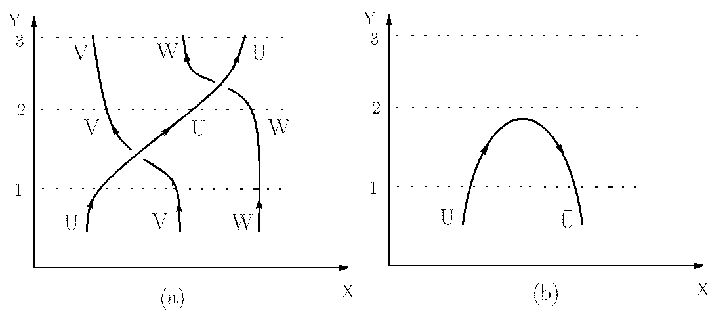
Then at the moment it will turn into . At the same time it should be something made from reordered product . The natural guess is
| (6) |
and, looking at the propagator (3), we understand that
| (7) |
with and somehow deformed r.h.s., because regularization can and do modify the naive answer. In the last expression Similarly, if the third operator is involved, then we get
| (8) | |||||
and so on. At the turning point we have a transition Fig.1(b)
| (9) |
from a pair of operators into an empty state.
Entire knot can be described as a transition from an empty state at to an empty state at with the associated amplitude, made from a product of and factors. For this product to transform under Reidemeister moves as vev of a Wilson loop the elementary factors should satisfy some bilinear and trilinear relations see s.3, the main one being the Yang-Baxter equation for . Then (7) implies that is the quantum universal -matrix of [64]-[73]. For such choice of the operators with the property (6) do indeed exist: the simplest example being the group elements of [65]. As explained in the introduction, it remains to understand why the regularized open Wilson lines (5) have the same commutation relations (7) – and this is beyond the scope of the present paper. Note that understanding of this fact is important for Chern-Simons theory, but is not really needed for building knot invariants: just instead of referring to the ”obvious” topological invariance of Wilson-line correlators in CST one needs to prove invariance of the product explicitly - and this will be done explicitly in s.4 below.
3 Operators arising from CST in temporal gauge
The invariance of vevs of Wilson loops under topological deformations imposes several conditions on the operators arising from CST in the temporal gauge. The purpose of this section is to argue that there are only two independent operators from which the vevs of Wilson loops can be constructed. We also derive the equations for these operators that ensures the topological invariance of vevs.
3.1 Projected knots
If additional flag structure on the space is fixed, then according to sections 1 and 2 we suppose that the answer for vev of a Wilson loop has the following properties:
- •
The answer is formulated in terms of a projection of a knot to a fixed plane . For definiteness, we specify this plane to be -plane in some reference frame.
- •
The answer gets angle-independent contributions only from crossings of the resulting two-dimensional curve and its turning points with respect to the fixed direction in the plane. We specify this direction to be -direction in our reference frame. This means that we need the universally defined operators corresponding to the crossings and the turning points. The vevs of Wilson loops are just appropriate contractions of these operators.
- •
Under topological deformations these contractions are transformed exactly as vevs of Wilson loops in CST.
With these desired properties in mind, let us consider a two-dimensional projection of a knot to the fixed plane, for example as in the Fig.2() . The arrows denote the orientation of the knot. Without loss of generality, we assume that all crossings of the resulting two-dimensional curve have two upper and two lower legs about fixed -direction. For example in the Fig.2() , are upper and , are lower legs. Obviously, every crossing can be reduced to this form by a small deformation in the plane.

We can see that for every two-dimensional projection only types of crossings, which differ from each other by orientation and types of turning points about direction can appear (see Fig.3).

According to the second property from of our list, we define corresponding crossing operators and operators for each type of turning point . The indices of these operators correspond to free legs of the crossings and the turning points in the two-dimensional picture. We assume that the upper index denotes an incoming leg and the lower denotes an outgoing one. Therefore, the crossing operators have two upper and two lower indices, the turning point operators have one index of each type Fig.4.

The vev of a Wilson loop can be represented in the form of contractions of these operators. More precisely, to find the vev , we need to peak a two dimensional projection of the closed curve , then attach to every crossing and turning points corresponding operators and contract the indices according to the two dimensional diagram. For example, for unknot with the two-dimensional projection represented in the Fig.5 the result is:
| (10) |

The CST implies that the result does not depend on the choice of the projection and is invariant under smooth topological deformations. This property imposes several conditions on the crossing and turning point operators. In the rest of this section we analyze these restrictions and derive the fundamental equations (3.6) for the special point operators. These equations ensures that under topological deformations the resulting contractions of the operators have the same transformation properties as the vevs of Wilson loops.
3.2 Turning point operators
Simple topological consideration shows, that the four operators , are not independent. Indeed, the straight vertical line is topologically equivalent to a curved line with two turning points Fig.6. Then the topological invariance of vevs of Wilson loops in CST implies that the corresponding turning point operators are related by the inversion:
| (11) |

Therefore, in fact, there are only two independent turning point operators and , and the others can be expressed trough them:
| (12) |
3.3 Crossing operators
Similar topological arguments show that there are only two independent crossing operators. Indeed, let us consider the topological deformations represented in the Fig.7. The topological invariance of vevs of Wilson loops in CST implies that the crossing operators and can be expressed trough the first one :
| (13) | |||

If in Fig.7 under-crossings are changed to over-crossings then we have:
| (14) | |||
i.e. the crossing operators and can be expressed trough .
3.4 Reidemeister movies. Ambient topological invariants.
Two knots in are considered to be equivalent if one of them can be transformed into the other via smooth deformations in . This is the definition of ambient isotopy equivalence and two such knots are referred to as ambient isotopy equivalent. Relations (12)-(14) for crossing and turning point operators ensure that the vevs constructed from them do not depend on homotopic deformations of two-dimensional projection in the plane, i.e. on smooth deformations in the plane that do not change the total number of crossings of this projection. This is not enough, however, for the vev to be topological invariant. Indeed, different two-dimensional projections of some knot can have different topologies, for example different numbers of crossings. Therefore, different, non-homotopic two-dimensional projections can represent the same knot.
Fortunately, there is a simple way to find out if the two knots represented by their two-dimensional projections are ambient isotopy equivalent or not [37]:
Theorem (Reidemeister)
Two knots in
represented by their two-dimensional projections
and are ambient isotopy equivalent if and only if
can be deformed into via smooth deformations in
the two-dimensional plane and finite set of Reidemeister moves,
shown in Fig.8.

The quantities that depend only on equivalence classes of ambient isotopy, or equivalently, do not vary under smooth two-dimensional deformations and Reidemeister moves are referred to as the ambient isotopy invariants.
3.5 Temporal framing. Regular isotopy invariants.
Despite the topological nature of CST, the expectation values of Wilson loops in this theory are not ambient isotopy invariants [8]-[19]. This feature of CST is closely related to the self-linking problem and the framing procedure. In CST the vevs of Wilson loops are ill-defined quantities, and to define these quantities properly one can introduce a second, auxiliary contour , called framing of , which can be considered as a slight displacement of contour along a normal to vector field [1]. More concretely, the word ”slight” means that we replace the contour representing the knot by a narrow-width rope bounded by and . Two different choices of framing contour for straight line are presented in the Fig.9(). When auxiliary contour is chosen, then it makes sense to calculate the linking number between contours and and its non-Abelian generalizations - the normalized vevs of product of two Wilson loops in CST:
| (15) |
The normalization means that in perturbation theory only propagators with different ends attached to different contours and are taken into account. Therefore, there are no collapsible propagators, and the quantity (15) turns out to be well defined.
Roughly speaking, the CST describes the properties of
knots that are made not of a ”rope” but of a ”ribbon” bounded by
and . In this case an additional parameter comes into
the game. Namely, a ”rope” can be replaced by a ”ribbon” in many
different ways with different number of twists of the ”ribbon”
Fig.9(). The answer in CST depends only on this . To
fix the number of the ribbon twists, different framing fixing are
used. In the temporal gauge there exists a natural choice for
framing fixing. Namely, one can fix two dimensional plane and then only ribbons which
have non-perpendicular to this plane tangent planes at every point
are considered. We call this procedure - temporal
framing. The examples of knots in the temporal framing are
represented in the Fig.9() , here the fixed
two-dimensional plane is the plane of the page.

The ”Wilson-loop” calculations in CST depend on the definition of the framing. In what follows we assume that all quantities are represented in the temporal framing.
Now, it is obvious that in the temporal
framing the first Reidemeister move from Fig.8 is not
respected, because the ribbon with loop on it in the temporal
framing is not equivalent to a straight ribbon, but to a ribbon
with additional twist, see Fig.10

The equivalence of knot projections defined only
by the second and the third Reidemeister moves form Fig.8
is usually referred to as regular isotopy invariance, and
quantities that does not change under these moves are the so
called regular isotopy invariants. In this way, we see,
that the presence of the framing result in the fact that the vevs
of Wilson loops are not ambient but only the regular invariants of
knots.
It was shown in the Witten’s work [1] that the
shift of the framing contour by twists results in a simple
multiple for the vev of a Wilson loop:
This is a crucial observation that enables the CST to work. It means that although we must pick additional framing contour to make the vev well defined, we do not lose the information since we know how this vev changes a under change of framing. Explicit perturbative computations performed in [8] show that the first terms of expansion of are:
where is renormalization of the bare constant , is the value of quadratic Casimir of the gauge Lie algebra and is the representation carried by the Wilson loop. We see that the results of the calculations are in agreement with the following expression:
| (16) |
The difference between and is somewhat controversial point, usually one assumes that (here stands for the value of quadratic Casimir in the adjoint representation of the gauge group) like in WZNW theory [63]. For our guessing this is not very essential: in the following we use directly parameter irrespective of its exact dependence of the bare .
Therefore, the CST generalizes the first Reidemeister move form
Fig.8 and the rest two remains unchanged. Finally, we can
infer that the vevs of Wilson loops have the transformation
properties summarized in the Fig.11

3.6 The fundamental equations
Let us analyze the restrictions imposed by generalized Reidemeister moves Fig.11 on the crossing and the turning point operators. First of all, we note that using the relations (12)-(14) we can express the crossing operators through and , similarly, the turning point operators are expressed trough and . Therefore, the resulting restrictions on the crossing and turning point operators can be reduced to equations on and . In terms of and the second Reidemeister relation in Fig.12 can be expressed as:
| (17) |
The first relation in Fig.12 means that:
| (18) |
or, equivalently:
| (19) |
where denotes the trace over the second space in the tensor product and we denote:
| (20) |
In terms of the ”down-directed” crossings corresponding to the operator in Fig.12(3) third Reidemeister move implies that satisfies the following trilinear equation:
| (21) |
It is easy to check that all other possible orientations of the crossings in the third Reidemeister relation Fig.11 (3) can be reduced to (21) by transformations (13) and (14). For this reason only (21) should be considered. Introducing the notations for the operators, acting in the triple product , we can rewrite this equation in the form:
| (22) |
This is the famous quantum Yang-Baxter equation (QYBE), arising in a number of physical and mathematical topics, from exactly solvable statistical models [67] to quantum groups [64]-[70]. Therefore, to describe the properties of vevs of Wilson loops in the CST the crossing and the turning point operators must satisfy two fundamental equations:
Solution of these equations is a pair of operators acting in appropriate tensor products of gauge group representations. With such a solution at hand, one can construct all crossing operators with the help of relations (13), (14) and (17). On the other hand side the pair satisfying (3.6) does not define the turning point operators but only the product of two operators (20). There is no additional relation between and imposed by topological moves and arbitrary choice of and satisfying (20) is possible. For instance, one can consider the following choice:
what means that the turning point operators and are identity operators due to (11) and do not give contribution to vev of Wilson loops and therefore, the corresponding turning points are not taken into account. In what follows we, however, assume the following relation:
| (29) |
This choice of additional relation is for the sake of symmetry
as it makes all the four turning point operators and turning points
equivalent. When added to (13), (14), (11), the relation (29) allows to
construct all crossing and turning point operators from given
solution of fundamental equations.

4 Universal quantum -matrix
As it was shown in the previous paper [34], the use of the naive propagator (3) leads to the crossing operator of the form:
| (30) |
where is the symmetric group of -elements, is a representation carried by a Wilson loop and . The universal, representation independent, form of (30) is:
| (31) |
where is the universal enveloping algebra of . Unfortunately, such crossing operator (31) does not satisfy the QYBE (22), what indicates that mote accurate regularization of propagator is necessary. Obviously, such a regularization of the naive answer should deform (31) somehow. In this section we make an obvious suggestion that this deformation of (31) is given by the well known quantum universal -matrix that seems to be in accordance with [36, 42, 62]. The quantum universal -matrix is not the element of anymore but the element of , where the algebra is the -deformed, or the quantized universal enveloping algebra of . In the subsections 4.1-4.3 we remind explicitly definition of and . In the subsection 4.4 we give the explicit expression for the universal quantum -matrix , then define the element and prove that these elements satisfy the fundamental equations (3.6).
4.1 Universal enveloping algebras
Let be a simple Lie algebra of rank with the root system
. Denote by the subset of positive roots and by
be the number of positive roots. Fix the set of
simple roots ,
and let be the set of elements
dual to the roots elements:
| (32) |
Here ( , ) is the Killing form reduced to the Cartan subalgebra. Let be a Cartan-Weil basis of . The Cartan matrix of the algebra is defined as . For arbitrary element from the Cartan subalgebra, we define the corresponding elements of the algebra as follows:
| (33) |
In particular, we will need the elements , and the element where is the half-sum of all positive roots:
| (34) |
The universal enveloping algebra of is the quotient of the tensor algebra by the ideal generated by the elements :
| (35) |
According to the Serre’s theorem this algebra can be defined as the algebra generated by elements with the following relations11 1 Note, that our choice of Cartan elements is different from the conventional one by the factor .:
| (36) |
| (37) |
| (38) |
| (39) |
The possible choice of a basis in is
given by the following Poincaré-Birchoff theorem:
The elements
form a basis of the universal enveloping algebra .
4.2 Quantized universal enveloping algebras
Let be indeterminate number, then the quantized universal enveloping algebra is the algebra with over , generated by elements subjected to the relations:
| (40) |
4.3 Braid groups and root elements
If is the Cartan matrix of a Lie algebra , then the numbers can take values or . Let be equal to or when is equal to or respectively. The Weil group is defined by reflections corresponding to the simple roots of satisfying the following relations:
| (45) |
Let be the longest element of the Weil group i.e. the element that has the longest length of its reduced decomposition (length of this element is equal to the number of positive roots for every Lie algebra). An important property of is that the sequence:
| (46) |
exhaust all positive roots of and defines
the ordering on the set
. Therefore, the Weil group and a fixed reduced
decomposition of a longest element allow to define
all root elements of starting from simple roots.
In the definition of enter only elements
and corresponding to simple
roots. To define the elements of corresponding to the
non-simple roots we need a notion of quantum Weil group
or Artin braid group.
The Artin braid group associated with is the
group generated by elements
with the following relations:
| (47) |
The braid group acts by automorphisms on [70]:
| (48) | |||
| (49) | |||
| (50) |
Let us define the roots of as in (46), then we define the root elements of as follows:
| (51) |
The following analog of Poincaré-Birchoff
theorem gives a basis in
:
The elements
form a basis of .
For a proof see [70].
4.4 Universal quantum -matrix
Let and , are the root elements of then the universal quantum -matrix is defined as an element of by the following explicit expression:
Here is the permutation operator: and the arrow above the product implies that the factors appear in the order defined by a reduced decomposition of longest elements of Weil group (46). The q-exponent is defined as:
The crucial property of the universal quantum -matrix is that
this matrix represents suitable regularization of the crossing
operator
(31). More precisely:
Proposition: The pair , where is the universal quantum -matrix (4.4) and is defined by the following explicit expression:
| (56) |
satisfies the fundamental equations,
(3.6).
Proof: The proof of the quantum Yang-Baxter
equation (the second fundamental equation) can be found in any
textbook on quantum group theory,see for example [65] or
[70]. The proof of the first fundamental equation in
(3.6) is a relatively long but direct computation:
| (57) | |||
| (58) | |||
| (59) | |||
| (60) | |||
| (61) | |||
| (62) | |||
| (63) |
Here we used the following facts and identities:
and is by definition the quadratic Casimir element of the algebra :
| (64) |
The proof for is analogous.
Now, having the solution of fundamental equations one can construct all the special point operators. The crossing operators are expressed trough the universal -matrix by (13), (14) and (17). To construct the turning point operators we need to pick up the operators , and satisfying (29). The obvious choice is:
then the rest of the turning point operators are expressed trough these two by (12). Explicit expressions for these operators are summarized in (5.1) and (5.1).
5 Knot invariants
The crossing and turning point operators introduced in the previous sections allow to calculate the ambient and regular knot invariants. In this section we describe in detail the procedure for computation of these invariants and give examples of these calculations for several different choices of the gauge group and its representation.
5.1 Regular knot invariants.
Let be a two-dimensional projection of a knot (here is the projector to the plane). Then the image is a closed planar curve with finite number of self-crossings and turning points about some distinguished direction in the plane. To compute the regular isotopy invariant we should reduce all crossings of to one of the 8 canonical crossings represented in Fig.3 (additional turning points can appear during this process). Then, we attach to every special point the corresponding operator, for example as in the Fig.13. The indices of these operators correspond to the incoming and outgoing lines of special points, therefore, the closed curve naturally defines the contraction of the indices of the operators. For instance such a contraction for the two-dimensional projection of the knot represented in Fig.13 reads:
| (65) |
If a Wilson loop is in a representation of a gauge group , then the operators of special points Fig.4 read:
where is the universal quantum -matrix (4.4) for . For example in the case of and is the fundamental representation, the contraction (65) gives:

5.2 Writhe number. Ambient invariants.
As it was discussed in the section 3.5 the quantity can be considered as an invariant of embedding of a ribbon into three-dimensional space. The knot is defined as and is a framing contour of introduced by regularization of CST. The quantity depends on the number of twists on a ribbon Fig.9(a), this results in the fact that it is not an ambient isotopy invariant of the knot, but only a regular invariant. Nevertheless, we can easily construct the ambient isotopy knot invariant using the quantity . Indeed, let is the total number of twists of a framing ribbon embedded in , this quantity is referred to as a writhe of the ribbon. According to (16), additional twist on the ribbon changes the vev of a Wilson loop for a factor . Therefore, the quantity defined as:
| (86) |
is an ambient
isotopy invariant. Here
stands for the vev of unknot and we divide by its value for normalization.
In the temporal gauge is the total number
of twists of a ribbon in the temporal framing introduced in the
section 3.5. The temporal framing is the procedure that
naturally defines the class of ribbon embeddings
for a given two-dimensional projection of the knot
. Therefore, one can define the writhe of a knot projection as
the writhe of its temporal framing ribbon:
| (87) |
It is rather obvious, that this definition is correct,
i.e. it does not depend on the choice of representative framing
ribbon. As a function of the writhe (87) has a
constructive representation in terms of itself. Indeed, every
crossing of is equivalent up to the planar rotations to one of
the two crossings represented in Fig.14

Define the writhes of these crossings as
| (88) |
Then the writhe (87) can be expressed as sum of writhes:
| (89) |
where sum runs over all crossing of .
5.3 Braid representation of the knots.
A useful way for representing knots is to make use the braid group . The Artin braid group (the braid group corresponding to the root system in terms of section 4.3) of strings is the group generated by generators satisfying the following relations:
| (90) | |||
Let be a representation of some quantum universal enveloping algebra, then one can construct associated representation of the braid group by the following explicit definition:
The first defining relation (90) in this representation is
obvious, and the second one simply follows from QYBE (22).
Each elements of admits a graphical representation. One can
associate to the element the picture shown in
Fig.15 (a), then the element can be represented as in the Fig.15(b):

i.e. can be considered as a twist of and string on the set of strings. The closure of the element is a two-dimensional diagram obtained by connection the endpoints of the strings of in a order preserving way Fig.16 (a):

Every link and knot in particular, can be represented as a
closure of an element
(this element and group are not uniquely defined). For
instance the simplest knot can be represented as a
closure of Fig.16(b). The braid
representation of knots provides useful tool for calculation of knot invariants
(86).
Indeed, applying the method for calculation of described in the
sections 5.1-5.2
to a closure of we arrive to the following
proposition:
Let knot be represented as a
closure of some element of a braid group .
Then an ambient isotopy invariant of a knot for gauge group
and representation is
given by the following explicit formula:
where is a writhe of the diagram associated with and
| (95) |
In the braid representation of a knot , every string of has only two turning points with respect to the vertical direction of the page. This is why the contribution of turning points appears in (5.3) in the form . The calculation of (5.3) for some particular knot is just a matter of multiplication and taking a trace of relatively big matrices. In the next subsection we give several explicit examples of such calculations of the knot invariants for first five nontrivial knots. We also give explicit expressions for and for different groups and their representations.
5.4 Explicit examples
In this section we give examples of explicit calculations of knot invariants and universal -matrix (4.4) for several particular groups and their representations. The invariants are calculated for the first five non-trivial knots from Rolfsen table [60] : and . The two dimensional projections of these knots with the temporal framing contour can be chosen as in the Fig.17:

The braid representations of these knots and the writhe numbers of the corresponding closures are summarized in the table:
5.4.1 representations of the weight .
The polynomial knot invariants arising from vevs of Wilson loops
carrying arbitrary representation of the group is a very
instructive example for application of general formulas of
sections 3-4. For this reason let us consider in
detail the construction of quantum generators for
and universal -matrix (4.4) in the case of representation
with highest weight .
The algebra is the tree-dimensional Lie algebra
with generators , and subjected to the following
relations:
All irreducible finite-dimensional representations of is the representations of highest weight . The dimension of the representation with highest weight is given by . In a suitable basis in the generators , and are represented by matrices with the following elements:
To get from Lie algebra generators of to the quantum group generators , and we replace the matrix elements of and by their quantum deformations:
where
It is a simple exercise to check that for arbitrary these matrices satisfy the relations (40)-(43) for :
| (117) |
Note, that in the representation of weight the generators and are subjected to the additional relation:
| (118) |
Therefore, in this case, the universal quantum -matrix (4.4) is given by the following finite sum:
| (119) |
The operator (56) in this case reads:
| (120) |
For the quadratic Casimir element (64) we find:
| (121) |
Note that for vev of the unknot we have:
| (122) |
Therefore, the ambient isotopy invariant (5.3) for a knot, represented by the closure of , is:
Using the braid representations for first six non-trivial knots and their writhe numbers in the standard framing (5.4) we find that for fundamental representation this invariant gives the Jones polynomials of the knots:
For a general value of the highest weight we find:
where the following conventions are used:
| (147) |
The quantum Recah coefficients are:
| (148) | |||
where runs over all non-negative numbers, such that each q-factorial in the sum gets non-negative argument, and:
| (149) |
The polynomials (5.4.1) were obtained in [31] as traces of monodromies for the correlators of the associated Wess-Zumino conformal field theory.
5.4.2 in fundamental representation
The irreducible representations of are representations of the highest weight . Here we consider the case of the first fundamental representation corresponding to . In this fundamental representation the root elements of the quantum group have the following property:
and the universal -matrix (4.4) takes the form:
In the standard basis of this matrix can be expressed as:
The element (56) in the fundamental representation reads:
The quadratic Casimir element (64) is :
For the vev of the unknot in this representation we find:
| (150) |
Therefore the ambient isotopy invariant (5.3) in this case reads:
Using the braid representations (5.4) for first six non-trivial knots and their writhe numbers in the temporal framing we get:
where . In accordance with [1] these invariants are the HOMFLY polynomials [48] of the knots.
5.4.3 in fundamental representation
The root system of so(N) corresponds to for even and to for even N. In both cases the root system consist of a roots of two types with lengthes (long roots) and (short roots). In the fundamental representation the root elements of the algebra are nilpotent:
The universal -matrix (4.4) takes the form:
The explicit expression for quantum R-matrix is different for even and odd . In suitable basis for we have:
| (165) |
where
and
In the case of even we get:
| (166) |
where
The operator (56) in both cases is given by the following expression:
The quadratic Casimir element:
For the vev of unknot we get:
| (167) |
Therefore the ambient isotopy invariant (5.3) in this case reads:
Using the braid representations (5.4) for first six non-trivial knots and their writhe numbers in the temporal framing we get:
where and . In agreement with [32] these invariants are the Kauffman polynomials [43] of the knots.
5.4.4 in fundamental representation
The case of the group in fundamental representation is very similar to one. In appropriate basis for for universal -matrix we have:
| (184) |
where
The operator (56) is given by the following expression:
The quadratic Casimir element:
The vev of unknot in this case:
| (185) |
and for the ambient isotopy invariant (5.3) we get:
In this case we again obtain the Kauffman polynomial (5.4.3) for the following values of parameters and .
6 Conclusion
In this paper we explicitly described the knot invariants,
constructed from the universal quantum -matrix of arbitrary
simple (quantum) Lie algebra , and demonstrated that they are
indeed invariant under all relevant Reidemeister moves. The
operators, naturally associated with this construction are,
however, the group elements of in the sense of [65],
rather than the Wilson -exponents in the temporal gauge. The
group elements [65] and special point operators discussed in
this paper are made of the generators of quantum algebra.
For this reason, one of the most important problem is to realize
how the ”primordial” generators of a Lie algebra are transformed
into the quantum ones in the perturbation theory. This question
and way the group elements arise as the free-field representation
of these -exponents, presumably a la [63],
remains to be worked out. Also relation to many other descriptions
of knot invariants, associated with other gauge choices in
Chern-Simons theory, is left beyond the scope of the present paper.
We hope that the explicit expressions for crossing
operators (5.1) will help to understand better the
quantization of the CST in the temporal gauge. A possible step
toward solution of this problem is to derive the analog of the
Labastida-Pérez (LP) formula [24]. This formula expresses
the -th order of vev of Wilson loop in perturbation theory as
the trace , where the element is defined combinatorially by the crossings of two
dimensional projection of the knot. The summation in all
orders was done in [34] and the result was represented in the
form of contraction of the ”wrong” crossing operator
(30) over all crossings. Now, we are in a reverse
situation. We know the ”correct” answer for the crossing operator
(4.4) depending on . Expanding this answer in
powers of , one can find a proper analog of the LP formula.
This formula should provide some combinatorial analogs of
Kontsevich integral [58] for finite-type or Vassiliev
invariants [57]. This would also help to solve a
long-standing problem of combinatorial description of Vassiliev
invariants. From the CST site, the correct analog of LP formula
would give the properly regularized perturbation theory in the
temporal gauge.
Acknowledgements
The work was partly supported by Russian Federal Nuclear Energy Agency, Russian Federal Agency for Science and Innovations under the contract 02.740.5029 (A.Mor.) The work was also partly supported by RFBR grants 09-02-00393-a(A.Mor.,A.Sm.) and 07-02-00645(A.Mor.) by joined grants RFBR-CNRS 09-01-93106(A.Mor.), 09-02-93105-CNRSL(A.Sm.), 09-01-92440-CE(A.Mor.), 09-01-92437-CEa (A.Sm.), 09-02-91005-AFN(A.Mor.), 09-02-90493-Ukr,(A.Mor.) and by Russian president’s grants for support of scientific schools NSh-3035.2008.2 (A.Mor.) and NSh-3036.2008.2 (A.Sm.). A. Smirnov is also pleased to thank the ”Dynasty” foundation for support.
References
- [1] E.Witten, Commun. Math. Phys. 121: 351, 1989
- [2] M.F.Atiyah, New Invariants Of Three-Dimensional And Four-Dimensional Manifolds. in durhan 1987, rpoceedingsthe mathematical heritage of Herman Weyl 285-299
- [3] A.S.Schwarz, Lett. Math. Phys. 2:247, 1978 Comm. Math. Phys. 67:1, 1979; Abstract of the Baku Topological Conference 1987
- [4] Dror Bar-Natan, Edward Witten, Perturbative expansion of Chern-Simons theory with noncompact gauge group. Commun.Math.Phys.141:423-440,1991
- [5] Dror Bar-Natan, Perturbative aspects of the Chern-Simons topological quantum field theory. Ph.D. Thesis
- [6] Dror Bar-Natan, Perturbative Chern-Simons theory. J.Knot Theor.Ramifications 4:503-547,1995
- [7] Dror Bar-Natan, Wheels, wheeling, and the Kontsevich integral of the unknot. q-alg/9703025
- [8] E.Guadagnini, M. Martellini, and M. Mitchev, Perturbative Aspects of the Chern-Simons Field Theory. Phys. Lett. B227:111, 1989
- [9] E. Guadagnini, M. Mintchev, Recent developments in Chern-Simons theory and link invariants. Nucl.Phys.Proc.Suppl.16:588-590, 1990
- [10] E. Guadagnini, M. Martellini, M. Mintchev, Chern-Simons field theory and quantum groups. In ”Clausthal 1989, Proceedings, Quantum groups” 307-317
- [11] E. Guadagnini, The Universal link polynomial. Int.J.Mod.Phys.A7:877-946,1992
- [12] E. Guadagnini, M. Martellini, M. Mintchev, Link invariants from Chern-Simons theory. Nucl.Phys.Proc.Suppl.18B:121-134,1990
- [13] E. Guadagnini, Braid group representations and link invariants. Published in Johns Hopkins Workshp 1990:1-38
- [14] E. Guadanini, The Link polynomials of the Chern-Simons theory. , Phys.Lett.B251:115-120,1990
- [15] E. Guadagnini, M. Martellini, M. Mintchev, Braids And Quantum Group Symmetry In Chern-Simons Theory. Nucl.Phys.B336:581,1990
- [16] E. Guadagnini, M. Martellini, M. Mintchev, Chern-Simons Holonomies And The Appearance Of Quantum Groups. Phys.Lett.B235:275,1990
- [17] E. Guadagnini, M. Martellini, M. Mintchev, Chern-Simons Field Theory And Link Invariants. Published in Johns Hopkins Workshop 95:146, 1989
- [18] E. Guadagnini, M. Martellini, M. Mintchev, Chern-Simons Model And New Relations Between The Homfly Coefficients. Phys.Lett.B228:489,1989
- [19] E. Guadagnini, M. Martellini, M. Mintchev, Wilson Lines in Chern-Simons Theory and Link Invariants. Nucl.Phys.B330:575,1990
- [20] J.M.F. Labastida, Knot theory from the perspective of field and string theory. hep-th/0201038, and in the proceedings of International Europhysics Conference on High-Energy Physics, 2001, Budapest, Hungary, 12-18 Jul 2001
- [21] J.M.F. Labastida, Knot invariants and Chern-Simons theory , hep-th/0007152
- [22] J.M.F. Labastida, Knot theory from a Chern-Simons gauge theory point of view, hep-th/0002221
- [23] J.M.F. Labastida, Chern-Simons gauge theory: Ten years after, hep-th/9905057
- [24] J.M.F. Labastida, E. Perez, Combinatorial formulae for Vassilev invariants from Chern-Simons gauge theory, J.Math.Phys.41:2658-2699,2000, hep-th/9807155
- [25] J.M.F. Labastida, E. Perez, Kontsevich integral for Vassiliev invariants from Chern-Simons perturbation theory in the light cone gauge. J.Math.Phys.39:5183-5198,1998, hep-th/9710176
- [26] M. Alvarez, J.M.F. Labastida, E. Perez, Vassiliev invariants for links from Chern-Simons perturbation theory. Nucl.Phys.B488:677-718,1997, hep-th/9607030
- [27] M. Alvarez, J.M.F. Labastida, Primitive Vassiliev invariants and factorization in Chern-Simons perturbation theory, Commun.Math.Phys.189:641-654,1997, q-alg/9604010
- [28] M. Alvarez, J.M.F. Labastida, Numerical knot invariants of finite type from Chern-Simons perturbation theory. Nucl.Phys.B433:555-596,1995, hep-th/9407076
- [29] M. Alvarez, J.M.F. Labastida, Analysis of observables in Chern-Simons perturbation theory. Nucl.Phys.B395:198-238,1993, hep-th/9110069
- [30] A.Morozov and A.Rosly early 90’s, unpublished
- [31] R.K. Kaul, T.R. Govindarajan, Three-dimensional Chern-Simons theory as a theory of knots and links. Nucl.Phys.B380:293-336,1992, hep-th/9111063
- [32] Wu, Yong-Shi; Yamagishi, Kengo, Chern-Simons Theory and Kauffman Polynomials Int. Jour. of Mod. Phys. A:5, 1165-1195 1990
- [33] Tudor Dimofte, Sergei Gukov, Jonatan Lenells, Don Zagier, Exact Results for Perturbative Chern-Simons Theory with Complex Gauge Group , Journal-ref: Commun.Num.Theor.Phys.3:363-443,2009, hep-th/0903.2472
- [34] A.Smirnov, Notes on Chern-Simons Theory in the Temporal Gauge, hep-th/0910.5011, to appear in the Proceedings of International School of Subnuclar Shys. in Erice, Italy, 2009
- [35] R. Kashaev, N.Reshetikhin Invariants of tangles with flat connections in their complements.I. Invariants and holonomy R-matrices math/0202211
- [36] R. Kashaev, N.Reshetikhin Invariants of links with flat connections in their complements.II. Holonomy R-matrices related to quantized universal enveloping algebras at roots of 1 math/0202212
- [37] K. Reidemeister, Elementare Begrundung der Knotentheorie, Abh. Math. Sem. Univ. Hamburg 5, 24-32 1926
- [38] J.W. Alexander, Topological invariants of knots and links. Trans. Amer. Math. Soc.30:2, 275-306, 1928.
- [39] V.F.R. Jones, A polynomial invariant for knots via von Neumann algebras. Bull.Am.Math.Soc.12:103-111,1985
- [40] V.F.R. Jones, Hecke algebra representations of braid groups and link polynomials. Annals Math.126:335-388,1987
- [41] V.F.R. Jones, On knot invariants related to some statistical mechanical models. Pacific J.Math.137:311-334,1989
- [42] L.H. Kauffman, Knots and topological quantum field theory. In ”Manhattan 1993, Proceedings, Quantum topology” 137-186
- [43] L.H. Kauffman, Knots and physics. Singapore: World Scientific 538 p. (Series on knots and everything, 1), 1991
- [44] L.H. Kauffman, Knots, abstract tensors and the Yang-Baxter equation. In ”Florence 1989, Proceedings, Knots, topology and quantum field theories” 179-334
- [45] L.H. Kauffman, H. Saleur, Free fermions and the Alexander-Conway polynomial. Commun.Math.Phys.141:293-327,1991
- [46] L.H. Kauffman, From knots to quantum groups (and back). In ”Argonne 1990, Proceedings, Quantum groups” 1-32
- [47] L.H. Kauffman, State models and the Jones polynomial Topology 26, no. 3, 395407, 1987
- [48] P. Freyd, D. Yetter, J. Hoste, W.B.R. Lickorish, K. Millett, A. Ocneanu, A new polynomial invariant of knots and links., Bull.Am.Math.Soc.12:239-246,1985
- [49] V.G. Turaev, O.Y. Viro, State sum invariants of 3 manifolds and quantum 6j symbols. Topology 31:865-902,1992
- [50] V. G. Turaev Reidemeister torsion in knot theory UMN, 1986, V.41, 1 (247), 97147
- [51] N.Yu. Reshetikhin, V.G. Turaev, Ribbon graphs and their invariants derived from quantum groups. Commun.Math.Phys.127:1-26,1990
- [52] V.G. Turaev, Quantum invariants of knots and three manifolds. De Gruyter Stud.Math.18:1-588,1994
- [53] V.G. Turaev, The Yang-Baxter equation and invariants of links. Invent.Math.92:527-553,1988
- [54] N. Reshetikhin, V.G. Turaev, Invariants of three manifolds via link polynomials and quantum groups. Invent.Math.103:547-597,1991
- [55] L.D. Faddeev, R.M. Kashaev, Quantum Dilogarithm. Mod.Phys.Lett.A9:427-434,1994
- [56] R.M. Kashaev, Quantum dilogarithm as a 6j symbol. Mod.Phys.Lett.A9:3757-3768,1994
- [57] V.A. Vassiliev, Cohomology of knot spaces, Amer. Math. Soc. Providence,RI, 23-69, 1990.
- [58] M. Kontsevich, Advances in Soviet Math.16, part 2 ,137, 1993
- [59] I.A. Dynnikov, Three-Page Approach to Knot Theory. Encoding and Local Moves, Funkts. Anal. Prilozh. vol. 33, 25-37, 1999
- [60] http://katlas.org, The Rolfsen knot table
- [61] A.Morozov, String theory, what is it?, Sov. Phys. Usp. 35, 671-714, 1992
- [62] C. Kassel, M. Rosso, V. Turaev, Quantum groups and knot invariants, Panoramas et Syntheses, no. 5 1997
- [63] A. Gerasimov, A. Morozov, M. Olshanetsky, A. Marshakov, Samson L. Shatashvili, Wess-Zumino-Witten model as a theory of free fields, Int.J.Mod.Phys.A5:2495-2589,1990
- [64] R. Floreanini, A. Morozov, L. Vinet, q hypergeometric functions, quantum algebras and free fields, Theor.Math.Phys.98:259-265,1994
- [65] A.Morozov and L.Vinet, Free field representation of group element for simple quantum groups , Int.J.Mod.Phys.A13:1651-1708,1998, hep-th/9409093
- [66] A. Morozov, L. Vinet, q hypergeometric functions in the formalism of free fields, Mod.Phys.Lett.A8:2891-2902,1993, hep-th/9309026
- [67] R.Baxter, Exaclty solved Models in Statistical Mechaniks, Academic Press, London-New-Yok, 1982
- [68] V.G. Drinfeld, Hopf algebras and the quantum Yang-Baxter equation Sov.Math.Dokl.32:254-258,1985, Dokl.Akad.Nauk Ser.Fiz.283:1060-1064,1985
- [69] V.G. Drinfeld,Quantum groups. J.Sov.Math.41:898-915,1988, Zap.Nauchn.Semin.155:18-49,1986
- [70] A.Klimyk, K.Schmudgen Quantum groups and their representations, Springer-Verlag, Berlin 1997
- [71] C.Kassel Quantum Groups, Springer-Verlag, New-York 1995.
- [72] V.Chari, A. Pressley, A guide to quantum groups, Cambridge university press, 1994
- [73] S.Majid, Foundations of quantum group theory, Cambridge university press, 1994