Augmented Lattice Reduction
for MIMO decoding

We consider a MIMO system with $M$ transmit and $N$ receive antennas such that $M\leq N$ using spatial multiplexing. The complex received signal is given by

where $\mathbf{x}_{\cc}\in\mathbb{C}^{M}$, $\mathbf{y}_{\cc}$, $\mathbf{w}_{\cc}\in\mathbb{C}^{N}$, $\mathbf{H}_{\cc}\in M_{N\times M}(\mathbb{C})$. The transmitted vector $\mathbf{x}_{\cc}$ belongs to a finite constellation $\mathcal{S}\subset\mathbb{Z}[i]^{M}$; the entries of the channel matrix $\mathbf{H}_{\cc}$ are supposed to be i.i.d. complex Gaussian random variables with zero mean and variance per real dimension equal to $\frac{1}{2}$, and $\mathbf{w}_{\cc}$ is the Gaussian noise with i.i.d. entries of zero mean and variance $N_{0}$. We consider the coherent case where $\mathbf{H}_{\cc}$ is known at the receiver.
Separating the real and imaginary part, the model can be rewritten as

in terms of the real-valued vectors

and of the equivalent real channel matrix

Here $n=2N$, $m=2M$.
The maximum likelihood decoded vector is given by

where $\left\|\cdot\right\|$ denotes the Euclidean norm.

An $m$-dimensional real lattice in $\mathbb{R}^{n}$ is the set of points

where $\mathbf{H}\in M_{n\times m}(\mathbb{R})$. We denote by $d_{\mathbf{H}}$ the minimum distance of the lattice, that is the smallest norm of a nonzero vector in $\mathcal{L}(\mathbf{H})$. More generally, for all $1\leq i\leq m$ one can define the $i$-th successive minimum of the lattice as follows:

We recall that two matrices $\mathbf{H},\mathbf{H^{\prime}}$ generate the same lattice if and only if $\mathbf{H}^{\prime}=\mathbf{H}\mathbf{U}$ with $\mathbf{U}$ unimodular.
Lattice reduction algorithms allow to find a new basis $\mathbf{H}^{\prime}$ for a given lattice $\mathcal{L}(\mathbf{H})$ such that the basis vectors are shorter and nearly orthogonal. Orthogonality can be measured by the absolute value of the coefficients $\mu_{i,j}$ in the Gram-Schmidt orthogonalization of the basis, see the GSO Algorithm 1.

We recall the following useful property of GSO: the length of the smallest of the Gram-Schmidt vectors $\mathbf{h}_{i}^{*}$ is always less or equal to the minimum distance $d_{\mathbf{H}}$ of the lattice [15]. In other words,

A basis $\mathbf{H}$ is said to be LLL-reduced [14] if its Gram-Schmidt coefficients $\mu_{i,j}$ and Gram-Schmidt vectors satisfy the following properties:

1. 1.

   Size reduction:

   $$\left\lvert\mu_{k,l}\right\rvert<\frac{1}{2},\hskip 10.00002pt1\leq l<k\leq m,$$

2. 2.

   Lovasz condition:

   $$\left\|\mathbf{h}_{k}^{*}+\mu_{k,k-1}\mathbf{h}_{k-1}^{*}\right\|^{2}\geq\delta\left\|\mathbf{h}_{k-1}^{*}\right\|^{2},\hskip 10.00002pt1<k\leq m,$$

where $\delta\in\left(\frac{1}{4},1\right)$ (a customary choice is $\delta=\frac{3}{4}$).
The LLL algorithm is summarized in Algorithm 2. Given a full-rank matrix $\mathbf{H}\in M_{n\times m}(\mathbb{R})$, it computes an LLL-reduced version $\mathbf{H}_{\red}=\mathbf{HU}$, with $\mathbf{U}\in M_{m\times m}(\mathbb{Z})$ unimodular, and outputs the columns $\{\mathbf{h}_{i}\}$ and $\{\mathbf{u}_{i}\}$ of $\mathbf{H}_{\red}$ and $\mathbf{U}$ respectively.

We list here some properties of LLL-reduced bases that we will need in the sequel. First of all, the LLL algorithm finds at least one basis vector whose length is not too far from the minimum distance $d_{\mathbf{H}}$ of the lattice. The following inequality holds for any $m$-dimensional LLL-reduced basis $\mathbf{H}$ [3]:

where $\alpha=\frac{1}{\delta-1/4}$ ($\alpha=2$ if $\delta=\frac{3}{4}$).
Moreover, the first basis vector cannot be too big compared to the Gram-Schmidt vectors $\{\mathbf{h}_{i}^{*}\}$:

In particular, if $j=\argmin_{1\leq i\leq m}\left\|\mathbf{h}_{i}^{*}\right\|$,

In this section we briefly review existing detection schemes which use the LLL algorithm to preprocess the channel matrix, in order to improve the performance of suboptimal decoders such as ZF or SIC [19, 18, 4].
Let $\mathbf{H}_{\red}=\mathbf{HU}$ be the output of the LLL algorithm on $\mathbf{H}$. We can rewrite the received vector as $\mathbf{y}=\mathbf{H}_{\red}\mathbf{U}^{-1}\mathbf{x}+\mathbf{w}$.

• •

  The LLL-ZF decoder outputs

  $$\mathbf{\hat{x}}_{LLL-ZF}=Q_{\mathcal{S}}\left(\mathbf{U}\left(\left\lfloor\mathbf{H}_{\red}^{\dagger}\mathbf{y}\right\rceil\right)\right),$$

  where $\mathbf{H}_{\red}^{\dagger}=(\mathbf{H}_{\red}^{T}\mathbf{H}_{\red})^{-1}\mathbf{H}_{\red}^{T}$ is the Moore-Penrose pseudoinverse of $\mathbf{H}_{\red}$, $\left\lfloor\cdot\right\rceil$ denotes componentwise rounding to the nearest integer and $Q_{\mathcal{S}}$ is a quantization function that forces the solution to belong to the constellation $\mathcal{S}$.

• •

  The LLL-SIC decoder performs the QR decomposition $\mathbf{H}_{\red}=\mathbf{Q}\mathbf{R}$, computes $\widetilde{\mathbf{y}}=\mathbf{Q}^{T}\mathbf{y}$, finds by recursion $\widetilde{\mathbf{x}}$ defined by

  		$\displaystyle\tilde{x}_{m}=\left\lfloor\frac{\tilde{y}_{m}}{r_{mm}}\right\rceil,$
  		$\displaystyle\tilde{x}_{i}=\left\lfloor\frac{\tilde{y}_{i}-\sum_{j=i+1}^{m}r_{ij}\tilde{x}_{j}}{r_{ii}}\right\rceil,\hskip 20.00003pti=m-1,\ldots,1,$

  and finally outputs $\mathbf{\hat{x}}_{LLL-SIC}=Q_{\mathcal{S}}\left(\mathbf{U}\widetilde{\mathbf{x}}\right)$.

In this paragraph we will investigate the performance of augmented lattice reduction. We begin by proving that our method, like LLL-ZF and LLL-SIC, attains the maximum receive diversity gain of $N$, for an appropriate choice of the parameter $t$ in (6). The diversity gain $d$ of a decoding scheme is defined as follows:

where $P_{e}$ denotes the error probability as a function of the signal to noise ratio $\rho$.

In order to prove the previous Proposition, we will show that in the $(m+1)$-dimensional lattice $\mathcal{L}(\widetilde{\mathbf{H}})$ there is an exponential gap between the first two successive minima. Then, using the estimate (4) on the norm of the first vector in an LLL-reduced basis, one can conclude that in this particular case the LLL algorithm finds the shortest vector in the lattice $\mathcal{L}(\widetilde{\mathbf{H}})$ with high probability. This, in turn, allows to recover the closest lattice vector $\mathbf{Hx}$ to $\mathbf{y}$ in $\mathcal{L}(\mathbf{H})$ supposing that the noise $\mathbf{w}$ is small enough.
The following definition makes the notion of “gap” more precise:

We now prove the existence of such a gap under suitable conditions:

Figure 1 shows the performance of augmented lattice reduction for an uncoded $6\times 6$ MIMO system using $16$-QAM constellations.
Two versions of augmented lattice reduction with different values of the parameter $\varepsilon$ are compared. Clearly it is preferable to choose $\varepsilon$ as big as possible in order to minimize the probability $P\{\left\|\mathbf{w}\right\|>\varepsilon d_{\mathbf{H}}\}$. Version 1 corresponds to the choice $\varepsilon=\frac{1}{2\sqrt{2}\alpha^{m-\frac{1}{2}}}$, the highest value of $\varepsilon$ that verifies the hypothesis of Proposition 1. At the SER of $2\cdot 10^{-4}$, its performance is within $2.5\dB$ from ML decoding and gains $1.5\dB$ with respect to LLL-SIC decoding.
Version 2 corresponds to a value of $\varepsilon$ optimized by computer search (experimentally, this is around $2^{-\frac{m}{4}}$), whose performance is within $2.2\dB$ of ML decoding at the SER of $2\cdot 10^{-4}$. From now on, we will always consider this optimized version. For higher values of $\varepsilon$, we are not able to prove that the LLL algorithm finds the shortest lattice vector in $\mathcal{L}(\widetilde{\mathbf{H}})$. However, it is well-known that the LLL algorithm performs much better on average than the theoretical bounds predict.

In order to further reduce the distance from ML decoding, one can add MMSE-GDFE preprocessing, which yields a better conditioned channel matrix. Figure 2 shows the comparison of augmented lattice reduction with LLL-SIC detection, both using MMSE-GDFE preprocessing. At the SER of $10^{-4}$, augmented lattice reduction is within only $0.4\dB$ from ML performance and gains $2.3\dB$ with respect to LLL-SIC decoding.
The gain with respect to LLL-SIC decoding increases with the number of antennas: it is $3.5\dB$ for an $8\times 8$ MIMO system, at the SER of $10^{-4}$. On the other side, augmented lattice reduction is still within $0.8\dB$ from ML performance (see Figure 3).

A lattice-reduction aided detection technique based on an augmented matrix similar to (6) (after MMSE-GDFE preprocessing) has been proposed in [12]. However, the philosophy behind the method of [12] is quite different: the parameter $t$ is chosen in such a way that the Lovasz condition on the last column of the augmented matrix is always verified. Specifically, considering the QR decomposition $\mathbf{H}_{\red}=\mathbf{QR}$ of the LLL-reduced matrix $\mathbf{H}_{\red}$, the condition $t>r_{m,m}$ is required. In general, this results in a much bigger value of the parameter $t$. Thus the transmitted message is detected from the last vector of the reduced augmented basis instead of the smallest basis vector.
On one side, this guarantees that the complexity increase is trivial because the only step required after reducing $\mathbf{H}$ is size reduction on the last column. On the other side, unlike our exponential gap technique, there is no guarantee that LLL reduction can find the required lattice vector. As a consequence, the performance of the decoder described in [12] is not as good, especially as the number of antennas increases; in fact it is about the same as LLL-SIC (see Figure 2). The authors then propose to use a quantization error correction to improve the performance, which requires an additional computational cost, and is not needed in our case.

The complexity of LLL reduction of a gaussian channel matrix $\mathbf{H}$ has been studied in [9]. As we have seen in Section II, every instance of the LLL-ZF (respectively LLL-SIC) decoder consists of three main phases:

1. 1.

   A full Gram-Schmidt orthogonalization is performed at the beginning of the LLL algorithm. This requires $O(nm^{2})$ elementary operations [7].

2. 2.

   The main ”while” loop of the LLL algorithm requires $O(m^{2})$ elementary operations for each iteration. The number $K(\mathbf{H})$ of iterations of the LLL algorithm for a fixed realization $\mathbf{H}$ of the channel is bounded by [9, 5]

   $$K(\mathbf{H})\leq m^{2}\log_{\frac{1}{\sqrt{\delta}}}\left(\frac{A(\mathbf{H})}{a(\mathbf{H})}\right)+m,$$

   (11)

   where $A(\mathbf{H})$ and $a(\mathbf{H})$ denote respectively the maximum and minimum norm of the Gram-Schmidt vectors of $\mathbf{H}$. For general $\mathbf{H}$, $K(\mathbf{H})$ can be arbitrarily large. However, it was shown in [9] that $\mathbb{E}(K(\mathbf{H}))\sim O\left(m^{2}\ln\left(\frac{m}{n-m+1}\right)\right)$.

3. 3.

   Finally, the ZF and SIC receiver entail respectively the multiplication by the pseudo-inverse of $\mathbf{H}_{\red}$ and its QR decomposition. Both have complexity order $O(nm^{2})$ [7].

For fixed $\mathbf{H}$, we can use the estimate (11) to obtain a bound of the number of iterations of the LLL reduction of $\widetilde{\mathbf{H}}$. The Gram-Schmidt orthogonalization of $\widetilde{\mathbf{H}}$ yields

In fact, the last Gram-Schmidt vector is the projection of $\begin{pmatrix}-\mathbf{y}\\ t\end{pmatrix}$ on the subspace

Therefore

LLL reduction increases the minimum of the Gram-Schmidt vectors [5], so $a(\mathbf{H}_{\red})\geq a(\mathbf{H})$, and $a(\widetilde{\mathbf{H}})\geq\varepsilon a(\mathbf{H})$. On the other side $t<a(\mathbf{H}_{\red})\leq A(\mathbf{H}_{\red})\leq A(\mathbf{H})$ and so $A(\widetilde{\mathbf{H}})=\max(t,A(\mathbf{H}))=A(\mathbf{H})$. Then

where $c=\log{\frac{1}{\sqrt{\delta}}}$. Following [9], we can estimate the average $\mathbb{E}[K(\widetilde{\mathbf{H}})]$, recalling that $\frac{A(\mathbf{H})}{a(\mathbf{H})}\leq k(\mathbf{H})$, the condition number of $\mathbf{H}$, and that [2]

We thus obtain

For the choice $\varepsilon=\frac{1}{2\sqrt{2}\alpha^{m-\frac{1}{2}}}$, the complexity of the main loop of the LLL algorithm using the new method is at most of the order of $O(m^{3})$.

Our complexity simulations evidence the fact that the upper bounds (11) and (12) on the average number of iterations of the LLL algorithm for LLL-aided linear decoding and the augmented lattice reduction method are both quite pessimistic. The number of iterations for both methods appears in fact to be almost linear in practice, see Figure 4.
We have chosen $\delta=\frac{3}{4}$ in all the numerical simulations.

While the number of iterations of LLL is indeed higher, approximately by a factor $2$, for the augmented lattice reduction (Figure 4), the total complexity expressed in flops⁴⁴ 4 Here we define a “flop” as any floating-point operation (addition, multiplication, division or square root). is about the same for LLL-SIC and the augmented lattice method (see Figure 5). The additional complexity of the LLL algorithm is balanced out by the complexity savings due to the fact that QR decomposition is not needed.

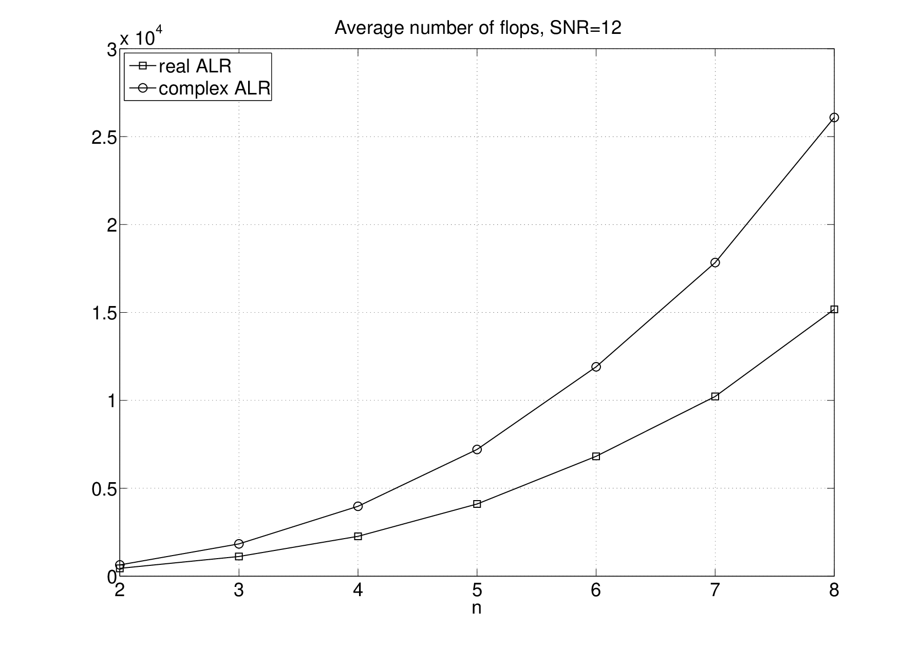
A generalization of the LLL algorithm to complex lattices has been studied in [16] and applied to MIMO decoding in [6]. It has been show experimentally in [6] that the complex versions of LLL-ZF and LLL-SIC decoding have essentially the same performance of their real counterparts but with substantially reduced complexity.
A complex version of the augmented lattice reduction can be implemented by LLL-reducing the $(N+1)\times(M+1)$-dimensional matrix

and allows to save about $40\%$ of computational costs (see Figure 6) without any change in performance.

References

- [1] L. Babai, “On Lovasz’ lattice reduction and the nearest lattice point problem”, Combinatorica, vol. 6, n.1, pp 1–13 (1986)
- [2] C. Chen, J.J. Dongarra, “Condition numbers of Gaussian random matrices”, SIAM Journal on Matrix Analysis and Applications, vol. 27, n.3 (2005), 603–620
- [3] H. Cohen, “A course in computational algebraic number theory”, Graduate Texts in Mathematics, Springer, 2000
- [4] M. O. Damen, H. El Gamal, G. Caire, “On maximum-likelihood detection and the search for the closest lattice point”, IEEE Trans. Inform. Theory. vol. 49, 2389–2402, 2003
- [5] H. Daudé, B. Vallée, “An upper bound on the average number of iterations of the LLL algorithm”, Theoretical Computer Science, vol. 123, n.1 (1994), 95–115
- [6] Y. H. Gan, C. Ling, W. H. Mow, “Complex Lattice Reduction Algorithm for Low-Complexity MIMO Detection”, IEEE Trans. Signal Process., vol 57 n.7 (2009)
- [7] G.H. Golub, C.F. Van Loan, “Matrix computations”, Johns Hopkins University Press, 1996
- [8] J. Jaldén, P. Elia, “DMT optimality of LR-aided linear decoders for a general class of channels, lattice designs, and system models”, submitted to IEEE Trans. Inform. Theory
- [9] J. Jaldén, D. Seethaler, G. Matz, “Worst- and average-case complexity of LLL lattice reduction in MIMO wireless systems”, IEEE International Conference on Acoustics, Speech and Signal Processing (ICASSP), (2008), 2685 – 2688
- [10] R. Kannan, “Minkowski’s convex body theorem and integer programming”, Math. Oper. Res. 12, 415–440 (1987)
- [11] K. Raj Kumar, G. Caire, A. L. Moustakas, “Asymptotic performance of linear receivers in MIMO fading channels”, submitted.
- [12] N. Kim, H. Park, “Improved lattice reduction aided detections for MIMO systems”, Vehicular Technology Conference 2006
- [13] C. Ling, “On the proximity factors of lattice reduction-aided decoding”, submitted.
- [14] A. K. Lenstra, J. H. W. Lenstra, L. Lovasz, “Factoring polynomials with rational coefficients”, Math. Ann., vol. 261, pp. 515-534, 1982
- [15] J. C. Lagarias, H. W. Lenstra Jr., C. P. Schnorr, “Korkin-Zolotarev bases and successive minima of a lattice and its reciprocal lattice”, Combinatorica, vol. 10 n.4 (1990), 333–348
- [16] H. Napias, “A generalization of the LLL-algorithm over Euclidean rings or orders”, Journal de Théorie des Nombres de Bordeaux 8 (1996), 387-396
- [17] M. Taherzadeh, A. Mobasher, A. K. Khandani, “LLL reduction achieves the receive diversity in MIMO decoding”, IEEE Trans. Inform. Theory, vol 53 n. 12, 2007, pp 4801–4805
- [18] C. Windpassinger, R. Fischer, “Low-complexity near-maximum likelihood detection and precoding for MIMO systems using lattice reduction”, Proc IEEE Information Theory Workshop, 2003, 345–348
- [19] H. Yao, G. W. Wornell, “Lattice-reduction-aided detectors for MIMO communication systems”, Proc. Global Telecommunications Conference 2002, vol 1, 424–428