Crossing Changes in Closed 3-braid Diagrams

There is a conjecture, due to Xiao-Song Lin, which states that the crossing shown in figure 2 is the only kind of nugatory crossing (This is problem 1.58 in [10]). In order to get a rigorous statement of this conjecture, we must first define exactly what we mean by a crossing change for a knot in $S^{3}$. Suppose $K$ is an oriented knot or link in $S^{3}$, and suppose we have a disk $D$ which intersects $K$ at exactly two points with opposite orientation. Such a disk is called a crossing disk for $K$. Suppose $D\times I$ is a bicollar of $D$ which intersects $K$ in a pair of arcs. There is a homeomorphism of $D\times I$ that fixes $D\times\{0\}$ and gives $D\times\{1\}$ a full rotation. Replacing $D\times I$ with its image under such a homeomorphism is called a crossing change. In [12] it is shown that this notion of a crossing change generalizes the notion of a crossing change in a specific diagram of a knot in the sense that a crossing change in a diagram determines a crossing change in $S^{3}$ and for any crossing change in $S^{3}$ one can find projections of the knot before and after the change that are identical except in a single crossing.

Using this definition of a crossing change, we can restate the conjecture as follows:

The union of these two disks produces a twice-punctured sphere which decomposes $K$ into a connected sum, although one of the summands may be trivial. This implies that there is a projection of the knot which looks like figure 2.

While this conjecture is still unproven, some partial results are known. Probably the most important of these states that the conjecture is true for the unknot. This follows from an argument of Scharlemann and Thompson, which uses the machinery of sutured manifold theory (see [12] for a proof). In [13], Torisu proved that 2-bridge knots satisfy the conjecture.

The conjecture is also known to hold for fibred knots, due to Kalfagianni [9].

The goal of this paper is to prove another special case of the conjecture. By examining the behavior of closed braids in Hecke algebras, we can prove the following:

The plan of the paper is as follows: First, we discuss the behavior of closed braids in a specific algebraic setting, the Iwahori-Hecke algebra. We describe an algorithm that inputs a closed braid and outputs a linear combination of the basis elements of the algebra. This algorithm gives us a way to better understand the form that a closed braid takes in the algebra. The full result requires the use of a powerful theorem of Birman and Menasco, known as the Markov Theorem without Stabilization, to generalize results about elements of the algebra back to closed braids.

Let $R$ be a domain. Fix units $A$ and $B$ in $R$ and fix an integer $n$. We define the Iwahori-Hecke algebra $H_{n}$ to be the associative $R$-algebra generated by $T_{1},\ldots,T_{n-1}$ and subject to the relations

• •

  $T_{i}T_{j}=T_{j}T_{i}$ if $|i-j|>1$

• •

  $T_{i}T_{i+1}T_{i}=T_{i+1}T_{i}T_{i+1}$

• •

  $T_{i}^{2}-BT_{i}-A=0$

There is a natural homomorphism from the braid group $B_{n}$ to $H_{n}$ given by $\sigma_{i}\mapsto T_{i}$, where $\{\sigma_{1},\ldots,\sigma_{n-1}\}$ are the standard generators of the braid group $B_{n}$. Thus $H_{n}$ is isomorphic to the group algebra $RB_{n}$ modulo the skein relation given in Figure 3 (which is implied by the third relation above).

The skein relation should be interpreted as follows: suppose $b_{+}$, $b_{-}$, and $b_{0}$ are braid diagrams which are identical except at a single crossing, where $b_{+}$ has a positive crossing, $b_{-}$ has a negative crossing, and $b_{0}$ has no crossing. Then the three diagrams are related in $H_{n}$ by the formula $b_{+}=Ab_{-}+Bb_{0}$.

The construction of $H_{n}$ given here follows the construction in [2]. The original construction was defined in [8].

$H_{n}$ is a useful setting for the study of braids, but since we are primarily interested in knots and links, one more step must be taken. Let $V_{n}$ be the quotient of $H_{n}$ by the extra relation $ab=ba$, where $a$ and $b$ are elements of $H_{n}$. Geometrically, this relation has the effect of replacing any braid diagram with its closure.

$V_{n}$ can now be described as an $R$-module of linear combinations of closed braid diagrams subject to the skein relations in figure 3.

Our first theorem gives some insight into the structure of $V_{n}$. Recall that a partition of a positive integer $n$ is a sequence of positive integers $(n_{1},\ldots,n_{m})$ such that $n_{1}\geq\ldots\geq n_{m}\geq 0$ and $n_{1}+\ldots+n_{m}=n$.

We can define an explicit basis for the $R$-module $V_{n}$. For a positive integer $k$, define $b_{(k)}$ to be the $k$-braid $\sigma_{k-1}\ldots\sigma_{2}\sigma_{1}$. Let $\lambda=(\lambda_{1},\ldots,\lambda_{m})$ be a partition of $n$. Define $v_{\lambda}$ to be the $n$-braid obtained by placing the braids $b_{(\lambda_{1})},\ldots,b_{(\lambda_{m})}$ side by side from left to right and regarding the whole as a single braid (see figure 4). The set $\{\hat{v_{\lambda}}\}$, where $\hat{v_{\lambda}}$ is the closure of $v_{\lambda}$ and $\lambda$ ranges over the partitions of $n$, is a basis for $V_{n}$.

The proof that $\{\hat{v_{\lambda}}\}$ is a basis will require an algorithm described by Bigelow in [2] and originally due to Hoste and Kidwell [7]. The purpose of this algorithm is to provide a systematic method for describing any closed braid in terms of this basis. The proof of Theorem 2 is provided in [2].

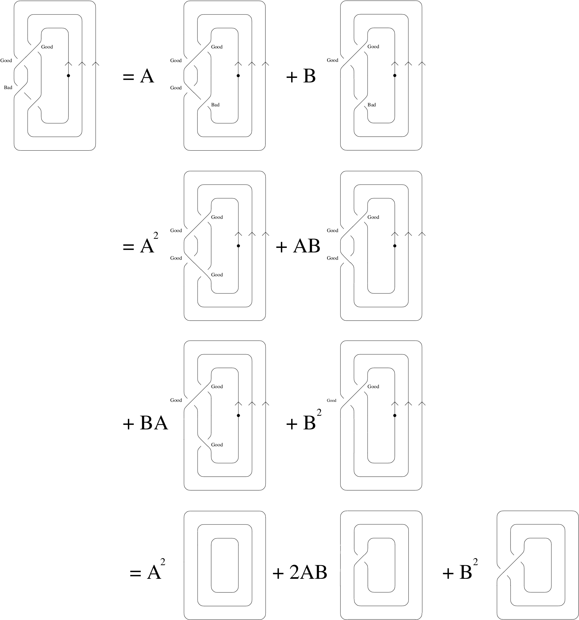
The algorithm itself is straightforward. Given a closed, oriented $n$-braid diagram, choose a basepoint anywhere on the braid that is not a crossing point. Isotope the braid by dragging a neighborhood of the basepoint toward the axis of the braid diagram, pulling it over all the other strands, so that the basepoint is at least as close to the axis as any other point. Consider every crossing in the diagram to be unlabeled. Starting at the basepoint, travel along the braid following its orientation. When an unlabeled crossing is encountered, we label it good if we are traveling along the overcrossing strand and bad if we are traveling along the undercrossing strand. See figure 5.

Whenever we encounter a bad crossing, we immediately use the skein relation to change our diagram into a linear combination of braid diagrams, one of which has replaced the bad crossing with a good crossing, and one of which has replaced it with no crossing. Using the same basepoint, we then run the algorithm on each of the resulting diagrams.

When we eventually travel back to the basepoint, we have obtained a diagram in which the component of the link containing the basepoint contains no bad crossings. In particular, this means that it contains only overcrossings with other components of the link. As such, we may isotope the entire component to the outer edge of the braid, moving it over all the other components, so that it is the farthest component of the link from the axis of the closed braid. We then apply the algorithm to any remaining components, choosing a new basepoint as necessary.

Once a crossing is labeled (and possibly changed) for the first time in this process, it will never again need to be changed. This is because a good crossing will always be labeled good in further iterations of the algorithm. The number of unlabeled crossings decreases with each iteration, and so the process will terminate in a linear combination of closed braid diagrams that contain no bad crossings. It is not difficult to see that the resulting diagrams must be braid isotopic to $\hat{v_{\lambda}}$ for some partition $\lambda$ of $n$.

An example of this algorithm is given below in figure 6.

This algorithm will be useful to us in the sections to follow, so it is to our benefit to make some remarks about it.

The MTWS is the result of an attempt to better understand the inner workings of Markov’s Theorem. While Markov’s theorem is is quite powerful and useful, especially when one is concerned with developing knot invariants using the machinery of braid theory, it does have a major drawback: given two braids which are Markov equivalent, Markov’s theorem does not supply an algorithm for changing one braid into the other using Markov moves. It does not even give any indication of how many moves may be required. For instance, it is possible that to change one 3-braid into another Markov equivalent 3-braid might require a sequence of a million consecutive stabilizations, a set of braid isotopies and conjugations, and a million consecutive destabilizations.

The MTWS does not directly provide an algorithm to transform one braid into another, but it does show that if such a transformation can be done, it can be done with a minimum of complexity. It does this by defining a new set of moves which are similar in flavor to Markov’s moves, but are required to to always be nonincreasing on braid index. Thus the sequences of intermediate braids between one braid and another are monotone decreasing on braid index. Together with a complexity function provided by the theorem, this creates an environment where we can study Markov equivalence between closed braids without worrying about the problem mentioned above (huge jumps in complexity).

In order to understand the terminology of the MTWS, a few definitions are in order.

A block-strand diagram is a diagram as in figure 9. When braids of the appropriate sizes are substituted into the blank boxes (called a braiding assignment), it becomes a closed braid diagram. Frequently, multiple parallel strands in a block-strand diagram are drawn as a single weighted strand, the number of intended strands being indicated next to the strand itself. Figures 9 and 10 include weighted strands to indicate that they can represent closed braids of any index. A template is a pair of block-strand diagrams $D$ and $E$, both with blocks $B_{1},\ldots,B_{k}$, together with an isotopy taking $D$ to $E$ in such a way that any fixed braiding assignment to the blocks yields closed braids $D^{\prime}$ and $E^{\prime}$ which represent the same knot type. Examples of templates are given below, which define the exchange and admissible flype moves listed in the statement of the MTWS. The destabilization move listed above is the same as the move given in Markov’s Theorem. All moves used in the MTWS preserve the knot type of the diagrams involved.

The MTWS gives us the tools necessary to prove the following key theorem.

Part of the reason this theorem is interesting is because it gives a new invariant of a subset of closed 3-braids, namely the output of the algorithm. Since one can apply trace functions to the algorithm’s output to get the HOMFLY polynomial, this invariant is potentially more sensitive than the HOMFLY and Jones polynomials. However, this invariant does not produce any new information about the knots with 10 or fewer crossings listed in [11] which have braid index 3.

References

- [1] S. Baader. Note on crossing changes. Q. J. Math., 57(2):139–142, 2006.
- [2] Stephen Bigelow. Braid groups and Iwahori-Hecke algebras. In Problems on mapping class groups and related topics, volume 74 of Proc. Sympos. Pure Math., pages 285–299. Amer. Math. Soc., Providence, RI, 2006.
- [3] Joan S. Birman. Braids, links, and mapping class groups. Princeton University Press, Princeton, N.J., 1974. Annals of Mathematics Studies, No. 82.
- [4] Joan S. Birman and William W. Menasco. Stabilization in the braid groups. I. MTWS. Geom. Topol., 10:413–540 (electronic), 2006.
- [5] Joan S. Birman and William W. Menasco. Stabilization in the braid groups. II. Transversal simplicity of knots. Geom. Topol., 10:1425–1452 (electronic), 2006.
- [6] Mikami Hirasawa and Yoshiaki Uchida. The Gordian complex of knots. J. Knot Theory Ramifications, 11(3):363–368, 2002. Knots 2000 Korea, Vol. 1 (Yongpyong).
- [7] Jim Hoste and Mark E. Kidwell. Dichromatic link invariants. Trans. Amer. Math. Soc., 321(1):197–229, 1990.
- [8] Nagayoshi Iwahori. On the structure of a Hecke ring of a Chevalley group over a finite field. J. Fac. Sci. Univ. Tokyo Sect. I, 10:215–236 (1964), 1964.
- [9] Efstratia Kalfagianni. Crossing changes of fibered knots, 2006. arXiv:math/0610440v3 [math.GT].
- [10] Rob Kirby. Problems in low dimensional topology. In Geometric Topology (Proc. Georgia International Topology Conference, University of Georgia, Athens, Georgia, 1993), Part 2, pages 35–358. Amer. Math. Soc., Providence, R.I., 1997.
- [11] Dale Rolfsen. Knots and links. Publish or Perish Inc., Berkeley, Calif., 1976. Mathematics Lecture Series, No. 7.
- [12] Martin Scharlemann. Crossing changes. Chaos Solitons Fractals, 9(4-5):693–704, 1998. Knot theory and its applications.
- [13] Ichiro Torisu. On nugatory crossings for knots. Topology Appl., 92(2):119–129, 1999.