Ordered spin structures of -MnO2 (rutile-type) systems with competing exchange interactions: numerical approach using equi-energy contour plot
Abstract
Using numerical calculations of equi-energy contour plot of the Fourier transform of the spin Hamiltonian, we study the magnetic phase diagram ( and ) of the rutile type -MnO2, where () is fixed and is the antiferromagnetic interaction along the diagonal direction, is the interaction along the axis, and is the interaction along the axis. The magnetic phase diagram consists of the multricritical point (the intersection and ), the helical order along the axis, the phase, the helical order along the axis, and the phase . The shift of the location of the magnetic Bragg peak in the reciprocal lattice plane is examined with the change of and in the phase diagram. The shift is discontinuous on the first-order phase transition, and is continuous on the second-order phase transition. The detail of our magnetic phase diagram is rather different from that reported by Yoshimori.
pacs
75.10.-b,75.30.KzI Introduction
It is well known that -MnO2 (with the rutile-type structure) is one of the systems with a helical spin order along the axis. Erickson[1] found from magnetic neutron scattering on -MnO2 that the spins are helically ordered with a period of 7 along the axis. The direction of spins in the plane turns from one plane to the next plane by an angle of (). In 1958, Yoshimori[2] theoretically demonstrated the origin and stability of the helical spin order in -MnO2, based on the experimental results from Erickson. The spin Hamiltonian of -MnO2 is described by a form of the Heisenberg-type, where the combination of nearest neighbor (n.n.) exchange interactions, next nearest neighbor (n.n.n.) exchange interactions, and so on are included. His success lies in the use of the Fourier transform of the spin Hamiltonian in the reciprocal lattice space. Then the Fourier transform depends only on exchange interactions and wavevectors Q. The location of the magnetic Bragg points in the reciprocal lattice space are uniquely determined from the condition that the Fourier transform takes a maximum.
In spite of the success in theory established by Yoshimori,[2] Erickson has not published his detailed data of the magnetic neutron scattering of -MnO2 as far as we know. Since 1958, there have been several papers on the magnetic structure of -MnO2 using magnetic neutron scattering[3, 4, 5] and magnetic x-ray scattering.[6, 7] In recent years, Sato et al, have reported that the magnetic Bragg peaks appear at the wave vector Q = (1, 0, 2 + ) in the units of (), (), and () in the reciprocal lattice space, where = 0.297 at 10 K, increases with increasing temperature, and reaches 0.2992 just below (= 92 K). The value of is rather different from 2/7 derived by Yoshimori.[2] This indicates that the helical spin structure along the axis is incommensurate with the - axis lattice constant.
Because of the crystal field (distorted octahedron formed by O2- ions) in the vicinity of Mn4+ ion, the ground orbital state of Mn4+ ion (, = 3 and = 3/2) is split into the () level (lower energy level, triple degenerate) and the () level (upper energy, double degenerate). As a result, the ground state is now orbital singlet, indicating that the orbital angular momentum is quenched. The electrons are responsible for the metallic conduction, while the localized electrons are responsible for the magnetism. In recent years, Sato et al.[8] have reported the transport properties of a single crystal -MnO2, such as electrical resistivity, thermopower, Hall effect, and magnetoresistance. Their data show an appreciable anomaly near . This implies that there is a strong correlation between conduction electrons and localized magnetic moment through the Hund’s rule. The DC magnetic susceptibility shows a significant deviation from a molecular-field theory based on a localized spin model, which was assumed by Yoshimori[2] on his helical spin order.
In the present paper, we study the magnetic phase diagram of -MnO2 type structure using the molecular field theory developed by Yoshimori,[2] where Mn4+ spins are localized. The exchange interactions along the diagonal axis of the system, along the axis and along the axis are taken into account. Note that is assumed to be fixed and be antiferromagnetic. According to Sato et al.,[8] the intra-atomic exchange interaction (Hund coupling), the transfer interaction between adjacent orbitals, and the occupancy of the orbitals are defined by , , and , respectively. Since and for -MnO2 (),[8] this means that the spin structure of -MnO2 below is not affected by the effect of and at al. In other words, the spin structure is well described by the localized spin model with , , and . We find that our magnetic phase diagram ( vs ) consists of four phases including the helical phase along the axis, the phase with (1/2, 0, 1/2), the helical phase along the axis, and the phase with (1, 0, 0). The detail of our phase diagram is rather different from that proposed by Yoshimori.[2] We use a numerical calculation approach in finding the distribution of the magnetic Bragg peaks in the fixed reciprocal lattice planes such as with one index fixed. To this end we calculate the equi-energy contour plot of the negative sign of the Fourier transform of the spin Hamiltonian, . The magnetic Bragg peaks are located inside the maximum equi-energy contour. The selection rule for the location of the magnetic Bragg peaks is the same as that derived by Yoshimori.[2] This numerical method has an advantage in visualizing the location of the magnetic Bragg peaks in the reciprocal lattice space. The nature of the phase transitions on the phase boundaries will be discussed.
II BACKGROUND: general theory for the ordered spin structure
We follow the theory presented by Nagamiya.[9] We consider a lattice of magnetic atoms such as -MnO2. The unit cell can be chosen so that it contains one magnetic atom. On each magnetic atom, we assume a classical spin. Between the spin at the position and at , there is an Heisenberg-type exchange interaction. The Heisenberg spin Hamiltonian is expressed by
| (1) |
where
and
The exchange interaction is not restricted to the nearest neighbors. We now use the Fourier transformations of the exchange interaction and spin;
| (2) | |||
| (3) |
with
where () is the total number of spins, and . The position vector is expressed by
where , , , and , , and are the fundamental lattice vectors. We also define the reciprocal lattice vector by
where b1, b2, and b3 are fundamental reciprocal lattice vectors and are given by
with
Noting that
we have
The periodic boundary condition for leads to
This means that the wavevector q is given by
where
For convenience we assume that
corresponding to the first Brillouin zone. There are wavevectors in the first Brillouin zone. The spin Hamiltonian is rewritten as
| (4) |
We look for the lowest minimum of Eq.(1) under the condition that
| (5) |
for any . Instead of this condition, we impose a milder condition
| (6) | |||||
where we use
Under this milder condition, the minimum of Eq.(1) is obtained simply by taking only that q for which has the maximum. Denoting this q by Q (q = -Q being equally allowed), we have the minimum value of Eq.(4) as
We also obtain
The condition (6) can be written as
for any . This indicates that
| (7) |
Here we assume that
where RQ and are real vectors.
| (8) | |||||
Then we have
Then the vector is perpendicular to the vector , and the magnitude is the same as the magnitude . From Eq.(8), we get
The minimum energy is obtained as
| (9) |
The spin vector is expressed by
where and are the unit vectors which are perpendicular to each other. For convenience, and are in the - plane. The axis is perpendicular to the - plane. Then using the unit vectors and , we get the final result
| (10) |
where is the angle between and axis.
The spin structure thus derived is the most fundamental spin structure and is realized as a result of the minimum energy state in the classical spin system. The ferromagnetic state () and antiferromagnetic state (Q = the zone boundary of the first Brillouin zone) are the special case of the spin structures. In general, Q is not related to the crystal structure, but is related to the details of the exchange interactions.
III Helical spin order for -
III.1 Calculation of for -MnO2
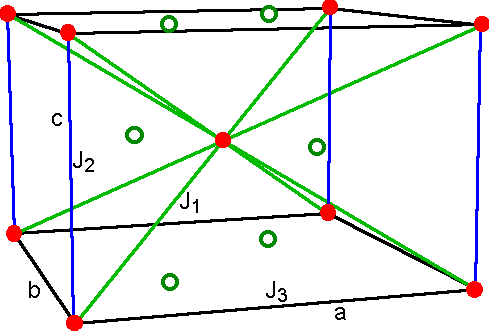
Figure 1 shows the structure (rutile) of -MnO2 where , , and .[8] The exchange interactions , , and are defined by Fig. 1. The definition of , , and are the same as that used by Yoshimori. The Néel temperature is equal to 92 K. Each Mn4+ ion and surrounding six O2- ions form a cation-occupied deformed octahedron (see Sec. X).
Here we calculate for MnO2, where the wavenumber q, the lattice vectors ( = 1, 2,…, 4) and c are given by
Then the expression of is given by
| (11) | |||||
Then can be rewritten as
where
with , , and being dimensionless numbers and and being reciprocal lattice constants.
III.2 Mathematica programs used in the present work
In order to determine the magnetic Bragg peaks in the reciprocal lattice plane, we use the following three Mathematica programs, ContourPlot for the equi-energy contour plot, FindMaximum for finding maximum, and ListVectorPlot3D for drawing the spin directions in the lattice points of the real space.
III.2.1 Contour plot program
This program is used to determine the overview on the positions of the magnetic Bragg peaks in the reciprocal lattice plane, where one of , , and are fixed. When the values of , , and are given, using the Mathematica program [ContourPlot], we can make a plot of the contours of (constant) in the plane, where the parameter is changed appropriately such that the maximum value of is obtained. This program is very useful to find the selection rule for the position of the magnetic Bragg peaks, as a function of , , and .
III.2.2 Finding maximum program
This program is used to determine the exact position of the magnetic Bragg peak in the reciprocal lattice plane, where one of , , and are fixed. For convenience, here we assume that is fixed such that = 0. Using the Mathematica program [FindMaximum], we find the maximum value of for given and , where (= -1) is fixed, and the regions of and are appropriately chosen. This program is very convenient when one wants to know how the position of the Bragg point changes as a function of and .
III.2.3 ListVectorPlot3D program
This program is used to draw the spin directions at each lattice sites in the real space. The spin structure depends on the values of Q.
IV Selection rule for the magnetic Bragg peaks from simple analysis
IV.1 Distribution of magnetic Bragg peaks in the (, , = fixed integer) reciprocal lattice plane
The magnetic Bragg peaks can be located at the wavevector q, where takes a maximum. When = fixed integer, is given by
suggesting that the location of the magnetic Bragg peaks in the (, , = fixed integer) reciprocal lattice plane depends only on and ,and is independent of the . The selection rule can be derived as follows.
(i) The distribution of the magnetic Bragg peaks is the same in the reciprocal lattice planes, (, , 1), (, , 3), (, , 5), (, , 7),…
(ii) The distribution of the magnetic Bragg peaks is the same in the reciprocal lattice planes , (, , 0), (, , 2), (, , 4), (, , 8),…
IV.2 Magnetic Bragg peaks along the direction with = fixed integer and
When = 0 and is a fixed integer, ( = fixed integer, = 0, ) is rewritten as
which indicates that the location of the magnetic Bragg peaks along the ( = fixed integer, = 0, ) direction depends only on and , and is independent of . The following selection rules can be derived.
(i) The location of the magnetic Bragg peaks along the direction is the same for (1, 0, ), (3, 0, ), (5, 0, ), (7, 0, ), .
(ii) The location of the magnetic Bragg peaks along the direction is the same for (0, 0, ), (2, 0, ), (4, 0, ), (8, 0, ), .
IV.3 Magnetic Bragg peaks along the direction with half inetgers
For half-integer (= 1/2, 3/2, 5/2, ), we have
leading to the appearance of the magnetic Bragg peaks appear at
for .
IV.4 Magnetic Bragg peaks along the direction
For any , can be expressed by
with . This indicates that the location of the magnetic Bragg peaks along the direction, is independent of . The derivative of with respect to is obtained as
Then we get the two solutions.
(i) Ferromagnetic or antiferromagnetic configurations
where
(ii) Helical spin configuration
under the condition of , where
The difference is calculated as
Then the helical spin order appears when
If the conditions and are satisfied, the magnetic Bragg peaks appear at the wavevectors denoted by
where is defined as
IV.5 Magnetic Bragg peaks along the direction
and its derivative are given by
and
respectively. Since in MnO2, we have only . Since , we have the following selection rule. The magnetic Bragg appears only at
along the -direction.
V Determination of and from experimental data on -
V.1 The ratio
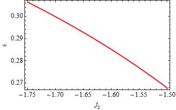
We now calculate the value of , at which takes a maximum, as a function of , where . The value of is uniquely determined as a function as shown in Fig. 2. When , we find (Yoshimori[2]).
Experimentally, the magnetic Bragg peak is observed at for -MnO2. Here we note that , where . The value of is slightly deviated from the value of 2 + 2/7, which is predicted by Yoshimori.[2] and its derivative are given by
and
respectively. has a maximum when
or
where
Since the magnetic Bragg peak appears at , we have
indicating that since .
V.2 Ratio
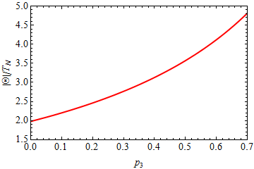
The ratio cannot be determined uniquely from the experimental results on the magnetic neutron scattering or x-ray magnetic scattering. The ratio can be calculated as
| (13) |
where , , is the Curie-Weiss temperature (the value is negative for -MnO2) and is the Néel temperature. The value of can be determined from the ratio since is already determined. We make a plot of as a function of in Fig. 3, where .
As far as we know, there have been several reports on the experimental values of and for -MnO2; K, K [Bizette and B. Tsai (1949)],[10] K, K [Ohama and Hamaguchi (1971)],[3] K, K [Sato et al.(2000)],[8] respectively. Using the values of , and the value of (= 1.68469) determined above, the value of can be calculated as = 0.537, 0.986, 1.091 using the data of Bizette and Tsai,[10] Sato et al.,[8] and Ohama and Hamaguchi,[3] respectively.
We note that the boundary of the helical phase is described by (the derivation will be shown later)
| (14) |
The helical order can exist only when . When for MnO2, should be lower than 0.5935. In other words, the ratio should be lower than 4.07853. Since K, this means that should be smaller than 375.2 K. The value of by Bizette and Tsai seems to be reasonable, while the values of obtained by Sato et al.[8] and Ohama and Hamaguchi[3] are much higher than 375.2 K. Note that Yoshimori[2] predicts that the boundary is described by . This expression is not correct according to our calculation.
VI Numerical calculation
VI.1 The contour plot of in the reciprocal lattice plane
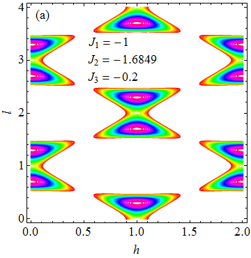
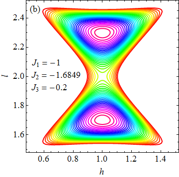

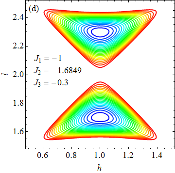
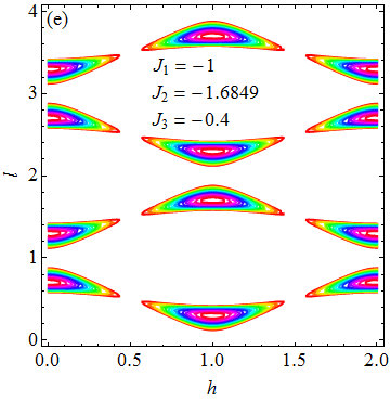
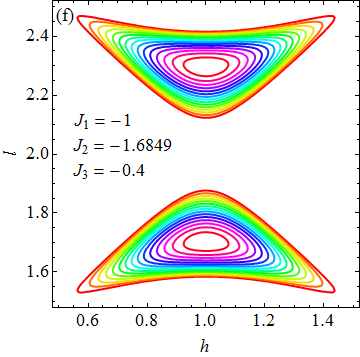
Using the numerical calculation of the contour plot using the Mathematica, we find the location of the magnetic Bragg peaks in the reciprocal lattice, where
takes a maximum, where , . Figures 4(a)-(f) show the contour plot of in the reciprocal lattice plane of , where () and is changed as a parameter (). As is predicted above, we find that the magnetic Bragg peaks appear at
where and is independent of (). Note that the essential results are independent of the choice of at least for .
VI.2 The contour plot of in the reciprocal lattice plane
Using the contour plot of the , we find the location of the magnetic Braggs in the reciprocal lattice, where
The location of the magnetic Bragg peaks is given by
in the reciprocal lattice plane of , where .
VI.3 The contour plot in the plane with
Using the contour plot of the Mathematica, we find the location of the magnetic Braggs in the reciprocal lattice, where
which does not depend on the index . Figures 5(a) show the location of magnetic Bragg peaks in the in-plane reciprocal lattice plane. We find that the magnetic Bragg peaks appear for even. This selection rule is true for with any integer .
VI.4 The contour plot in the plane with
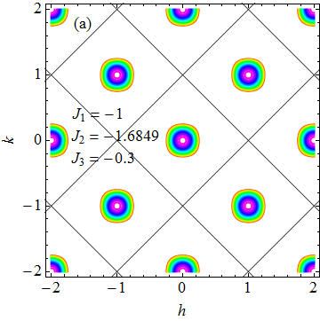
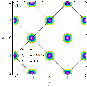
Using the contour plot of the Mathematica, we find the location of the magnetic Braggs in the reciprocal lattice, where
which does not depend on the index . Figure 5(b) show the location of the magnetic Bragg peaks in the in-plane reciprocal lattice plane, where is the integer. The magnetic Bragg peaks appear for odd for .
VII Phase diagram in the plane
The phase diagram for can be determined using the programs of the ContourPlot and FindMaximum. The phase diagram consists of the four phases; (i) the helical order along the axis, (ii) the helical order along the axis, (iii) the ordered phase with , , and , and (iv) the ordered phase with , , is shown in the phase diagram Fig. 6.
VII.1 Ordered phases
VII.1.1 Helical order along the axis
The spin vectors in the same plane are parallel, i.e., and . They screw along the axis. We find the maximum of
by taking the derivative of with respect to . The condition of the local maximum is given by
where . Then the maximum of is given by
| (15) |
for the helical order with (, , and ) where ,
VII.1.2 Helical order along the axis
The helical spin order where the spin vector in the same bc plane are parallel and they screw along the axis. We find the maximum of
by taking the derivative of with respect to . The condition of the local maximum is given by
where . The maximum value is
| (16) |
VII.1.3 The ordered phase with , , and
is given by
| (17) |
VII.1.4 The ordered phase with , , and
This phase corresponds to the MnF2-type antiferromagnetic structure (named by Yoshimori[2]). is evaluated as
| (18) |
VII.2 Boundaries between ordered phases
VII.2.1 The phase boundary between the spin order with the phase (, , and ) and the helical spin order along the axis
The difference of between the helical spin order along the axis and the phase is given by
So the helical ordered phase is energetically favorable when
with the condition of . When , this inequality can be rewritten as
| (19) |
or
VII.2.2 The phase boundary between the spin order with (, , ) and the spin order with (, , )
The difference of between the and the phase is given by
When
| (20) |
the phase is energetically favorable. When
| (21) |
the phase , , ) is energetically favorable.
VII.2.3 The phase boundary between the helical order along the axis and the phase (, and )
The difference of between the and the helical order along the axis is given by
Then the helical order is stable for . This inequality is satisfied for the condition of the helical order
VII.3 Multicritical point ( and ) and phase transition lines
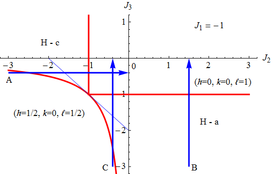
All four ordered phases merge only at the multicritical point at ( and ), where the line given by and the curve intersect with other (see the phase diagram of vs ). Note that . As will be shown later, the line () is of the first-order. The lines denoted by and are of the second-order.
(1) Using the program of finding maximum in for each point (, ) in the phase digram, we find the local maximum point in the - plane. The location of these points is plotted as a function of when is fixed and as a function of when is fixed.
(2) Using the program of finding maximum in for each point (, ) in the phase diagram, we find the local maximum point in the - plane. These points are plotted as a function of when is fixed and as a function of when is fixed.
VII.3.1 Scan A
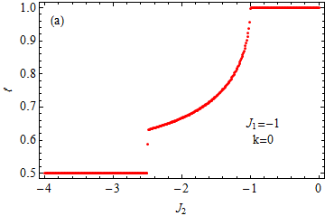
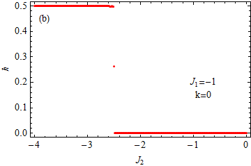
In the Scan A (see Fig. 6), we choose and . is changed as a parameter between and 0. We make a plot of vs in Fig. 7(a). The discontinuity in vs occurs at [the phase boundary (first order) between the phase with and the helical order along the axis], where the relation is satisfied (). We find that the relation of vs is well described by
| (22) |
for (the helical phase along the axis). For example, when , we have as shown in Fig. 7(a). We note that is equal to 1 at [the phase boundary(second order) between the helical phase along the axis and the phase with ] and remain unchanged () for . We also make a plot of vs in Fig. 7(b). The value of undergoes a sudden change from to 0 at (at the phase boundary between the phase with and the helical order along the axis) and remains constant () for . Note that there is no change of at .
VII.3.2 Scan B
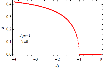
In the Scan B (see Fig. 6), we choose and . is changed as a parameter between -4.0 and 0. We make a plot of vs in Fig. 8. The value of decreases with increasing and reduces to zero at [the phase boundary (second-order) between the helical order along the axis and the phase with ]. We find that the relation of vs is well described by
| (23) |
The value of is independent of . For example, when , we have . The plot of vs (which is not shown here) indicates that remains constant () for , where .
VII.3.3 Scan C
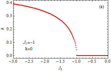
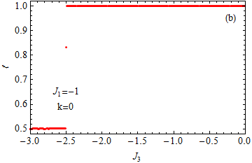
In the Scan C, we choose and . is changed as a parameter between -3.5 and 0. We make a plot of vs and vs in Figs. 9(a) and (b). As shown in Fig. 9(a), the value of decreases with increasing , showing an abrupt decrease at (which is denoted by ) [the phase boundary (first-order) between the phase with and the helical order along the axis]. The value of decreases with further increasing , following Eq.(23), and reduces to zero at [the phase boundary (second-order) between the helical order along the axis and the phase with ].
In Fig. 9(b), the value of increases with increasing . It shows an abrupt change from to at at the phase boundary (first-order) between the phase with and the helical state along the axis.
VIII Contour plot of for typical points in the phase diagram
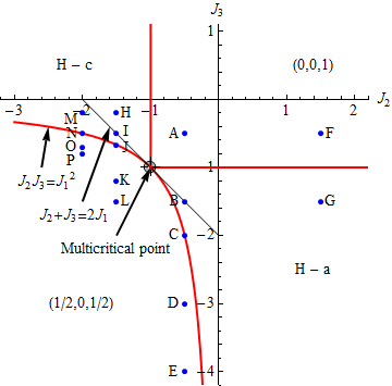
Here we show the contour plot of for the typical points in the (, ) phase diagram (see Fig. 10). The maximum points in the countour plot of ) correspond to the magnetic Bragg peaks in the plane.
VIII.1 The points A, B, C, D, and E with and


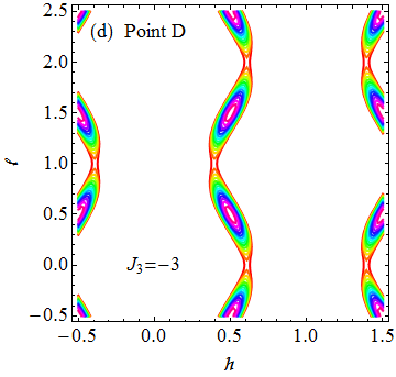
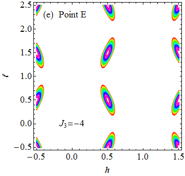
Typical contour plot of at the points A, B, C, D, and E in the (, ) phase diagram are shown in Fig. 11. The point A () is in the phase with ( = 0, = 0, = 1). The point B ( = -1.5) is in the helical phase with the axis. The point C () is the phase boundary between the phase with and the helical phase with the axis. The points D () and E () are in the phase with .
VIII.2 The points F and G with and .


Typical contour plot of at the points F and G in the (, ) phase diagram are shown in Fig. 12. The point F () is in the phase with . The point G () is in the helical phase with the axis.
VIII.3 The points H, I, J, K, and L with and
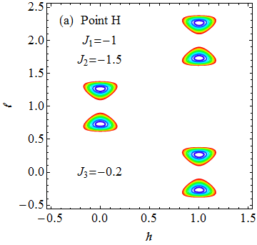


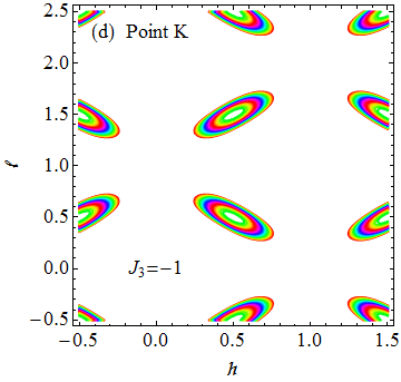
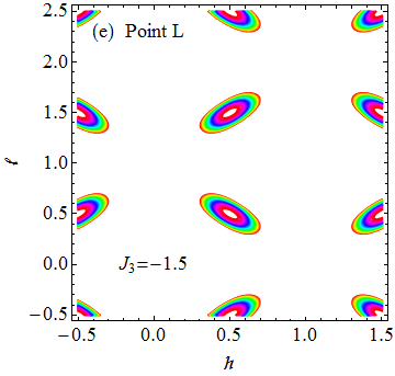
Typical contour plot of at the points H, I, J, K, and K in the (, ) phase diagram are shown in Fig. 13. The point H () is in the helical phase along the axis. The point I () is in the helical phase with the axis and is on the line (). The point J () is on the phase boundary between the helical phase with the axis and the phase with . The points K () and L () are in the phase with .
VIII.4 The points M, N, O, and P with and


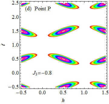
Typical contour plot of at the points M, N, O, and P in the (, ) phase diagram are shown in Fig. 14 The point M () is in the helical phase along the axis. The point N () is on the phase boundary () between the helical phase with the axis and the phase with . The points O () and P () are in the phase with .
IX 3D spin structures
What is the three dimensional (3D) spin structure which is characterized with the wavevector of the magnetic Bragg peaks? The vector of spin at the site of the real lattice space is given by
where , we assume that the phase factor is equal to zero, and Q is defined as
IX.1 Phase with
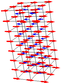
A typical spin structure for the phase with (0, 0, 1) is described in Fig. 15.
IX.2 Phase with
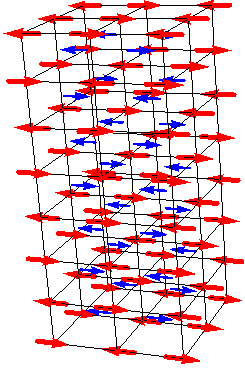
A typical spin structure for the phase with (1/2, 0, 1/2) is described in Fig. 16.
IX.3 Helical ordered phase along the axis;
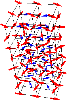
IX.4 Helical ordered phase along the axis (Yoshimori); commensurate structure
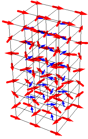
A typical spin structure with is commensurate with the lattice structure and described by Fig. 18. The magnetic unit cell along the axis is seven times larger than the unit cell of the crystal unit cell.
IX.5 Helical ordered phase along the axis:
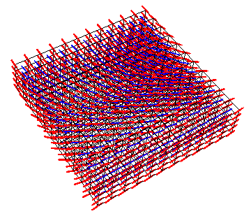
X Discussion: nature of exchange interactions in the rutile-type -
X.1 Overview
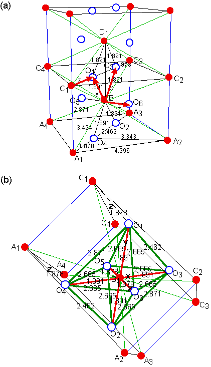
We show that the magnetic phase diagram with is uniquely determined by the combination of and , where the sign of is mainly negative and the sign of is changed between negative to positive. For -MnO2, we have and as , leading to and when . This point (, ) for -MnO2 is in the helical order along the axis, as shown in the magnetic phase diagram (Fig. 6).
In Fig. 20(a), we show the structure of -MnO2. Figure 20(b) shows the distorted octahedron where one Mn4+ ion (cation) at the point B1, is surrounded by six O2- ions (anion) at the points O1, O2, O3, O4, O5, and O6. The cation-cation separation (A1C1, B1D1) along a [001] axis is considerably smaller (). Because of the distorted octahedron formed by O2- ions in the vicinity of Mn4+ ion, the ground orbital state of Mn4+ ion (, and ) is split into the () level [lower energy level, triple degenerate; , , and states] and the () level [upper energy, double degenerate; , )]. The state is occupied by three electrons with spin up state . The state is empty. As a result, the ground state is orbital singlet, indicating that the orbital angular momentum is quenched. In -MnO2, the electrons are responsible for the metallic conduction, while the localized electrons are responsible for the magnetism. In Fig. 20(b), the orbital axis at the point B1 coincides with O5B1O6 (the axis). The axes coincide with O3B1O4 (the axis) and the O1B1O2 (the axis). The and axes are perpendicular to the axis. However, the axis is not perpendicular to the axis (, ).
X.2 Origin of the direct exchange interaction
We consider the exchange interaction between the points B1 and D1 (or between the points A1 and C1). The distance B1D1 (A1C1) is . In Fig. 20(b), one orbital () from the point B1 bisects the angle O1B1O3 and meets at the middle point of the edge O1O3. The other orbital from the point D1 (the center of neighboring octahedron) bisects the angle O1D1O3 and meets at the middle point of the edge O1O3. According to Goodenough,[11] the predominant interactions between neighboring cations whose cation-ccupied octahedra share an edge, are assumed to be direct cation-cation exchange interaction. Thus the interaction is antiferromagnetic (Heitler-London type) for -MnO2.
X.3 Origin of superexchange interaction
We consider the interaction between Mn4+ at the point B1 and the Mn4+ at the point C1 as shown in Figs. 20 (a) and (b), where the distance C1B1 is . According to Goodenough,[11] this interaction () is a superexchange one since the cation-occupied octahedra share a common corner (point O1). The angle C1O1B1 is equal to , this interaction is antiferromagnetic for -MnO2. According to Goodenough,[11] when the cation-occupied octahedral share a common corner, there can be no direct overlap of neighboring cation orbitals and therefore there is no cation-cation interactions.
What is the origin of ? The point C1 is the center of the neighboring octahedron. The direction of C1O1 is the axis of this octahedron. A orbital of O1 is expected to be directed toward C1 ( orbital) so as to overlap the orbital of the point C1, where the orbital (, , states) is called as orbital when the principal axis of the orbital coincides with the direction of the bond. A partial covalent bond between the orbital and the orbital can be formed. Then the charge transfer occurs from the orbital with the spin-up state to the state. Consequently, the spin of Mn4+ at the point C1 is still in the spin-up state, while the resulting spin of O2- at the point O1 is in the spin-down state. The remaining state at the point O1 is magnetically coupled with the state of the Mn4+ at the point B1. When this coupling (denoted as ) is antiferromagnetic, then the suprexchange interaction between Mn4+ at the point C1 and Mn4+ at the point B1 is ferromagnetic. On the other hand, when this coupling is ferromagnetic, then the superexchange interaction between Mn4+ at the point C1 and Mn4+ at the point B1 is antiferromagnetic. Here we note that the angle C1O1B1 is equal to for -MnO2, which is very different from . If , the orbital on the bond O1C1 coincides with the orbital on the bond O1B1 (the axis), where the orbital (, , states) is called as orbital when the principal axis of the orbital is perpendicular to the direction of the bond. The orbital is coupled with the state of the Mn4+ at the point B1, since the state is empty. According to the Goodenough-Kamamori-Anderson rule,[11, 12, 13, 14] the interaction is antiferromagnetic, since the orbital is not orthogonal to the orbital. If , the orbital is coupled with the orbital of the Mn4+ at the point B1 the interaction is ferromagnetic, since the orbital is orthogonal to the orbital.
The sign of is dependent on the value of . There may be a critical angle . is ferromagnetic for and is antiferromagnetic for . Experimentally, the superexchange interaction is antiferromagnetic for -MnO2, which means that is ferromagnetic. The critical angle is lower than .
The direct cation-cation exchange interaction () is expected to be stronger than the superexchange interactions . The competition between and can lead to a complicated compromise magnetic order; for -MnO2. Note that the discussion of Osmond[15] on the nature of may be inappropriate.
X.4 Origin of superexchange interaction
We consider the interaction between Mn4+ at the point A1 and the Mn4+ at the point A2, as shown in Figs. 20(a) and (b), where the distance A1A2 is . According to Goodenough,[11, 12] this interaction () is a superexchange one (cation-anion-cation) since the cation-occupied octahedra share a common corner (point O4). The angle A1O4A2 is equal to , the distance O4A2 is , and the distance O4A1 is . This interaction is experimentally antiferromagnetic for -MnO2; . This means that the critical angle is between and .
XI CONCLUSION
We have studied the phase diagram of ( vs ) with in the rutile type -MnO2 by using the equi-energy contour plot. The distribution of the magnetic Bragg peaks can be clearly visualized. The magnetic phase diagram consists of the multricritical point (the intersection and ), the helical order along the axis, the phase, the helical order along the axis, and the phase . The phase transition is of the first order between the phase and the helical order along the axis, and between the phase and the helical order along the axis. The phase transition is of the second order between the phase and the helical order along the axis, and between the phase and the helical order along the axis.
Acknowledgements.
We are grateful to Prof. H. Sato for useful discussions on the itinerant nature of electrons in -MnO2.References
- [1] R.A. Erickson, Phys. Rev. 90, 779 (1953).
- [2] A. Yoshimori, J. Phys. Soc. Jpn. 14, 807 (1959).
- [3] N. Ohama and Y. Hamaguchi, J. Phys. Soc. Jpn. 30, 1311 (1971).
- [4] M. Regulski, R.Przenioslo, I. Sosnowska, and J.-U. Hoffmann, Phys. Rev. B 68, 172401 (2003).
- [5] M. Regulski, R.Przenioslo, I. Sosnowska, and J.-U. Hoffmann, J. Phys. Soc. Jpn.73, 3444 (2004).
- [6] H. Sato, K. Wakiya, T. Enoki, T. Kiyama, Y. Wakabayashi, H. Nakano, and Y. Murakami, J. Phys. Soc. Jpn. 70, 37 (2001).
- [7] H. Sato, Y. Kawamura, T. Ogawa, Y. Murakami, H. Ohsumi, M. Mizumaki, and N. Ikeda, Physica B 329 – 333, 757 (2003).
- [8] H. Sato, T. Enoki, M. Isobe, and Y. Ueda, Phys. Rev. B 61, 3563 (2000).
- [9] T. Nagamiya, Solid State Physics, edited by F. Seiz, D. Turnbull, and H. Ehrenreich, 20, 305 (Academic Press, New York,1967).
- [10] H. Bizette and B. Tsai, Colloque sur la polarization de la matere cited by Lidiard (Paris, C.N.R.S., 1949) 164, Reports on Progr. in Phys. 17, 201 (1954).
- [11] J.B. Goodenough, Phys. Rev.117, 1142 (1960).
- [12] J.B. Goodenough, Magnetism and the Chemical Bond (John-Wiley & Sons, New York, 1963).
- [13] J. Kanamori, J. Phys. Chem. Solid 10, 87 (1959).
- [14] P.W. Anderson, Solid State Physics, edited by F. Seiz and D. Turnbull (Academic Press, New York and London, 1963) 14, 99.
- [15] W.P. Osmond, Proc. Phys. Soc. 87, 335 (1966).