A gauge mediation scenario with hidden sector renormalization in MSSM

The minimal supersymmetric standard model (MSSM) is an attractive framework of a theory beyond the standard model. It resolves some of the shortcomings of the standard model and at the same time makes falsifiable predictions for upcoming experiments. The presence of dark matter, for an instance, has been consolidated by numerous cosmological and astrophysical observations [1]. According to the best-fit $\Lambda$-cold dark matter (the ‘concordance’) model, the major part of the energy density of the present universe is dark energy and dark matter, neither of them is explained by the standard model. While dark energy is likely to be of gravitational origin, dark matter is readily accommodated in MSSM; as the lightest superparticle (LSP) is protected by R-parity, it is an ideal candidate of dark matter.

Among competing supersymmetry breaking scenarios of MSSM, the gauge-mediated supersymmetry breaking (GMSB) [2] is advantageous for natural suppression of flavor-changing neutral currents and CP violation. In GMSB the LSP is gravitino. Cosmological model building with successful structure formation favors cold dark matter, which, in the case of gravitino dark matter, yields gravitino mass lower bound $m_{3/2}\gtrsim 100$ keV. Gravitino LSP of this mass range is realized by GMSB models with sufficiently high messenger scale (see also Section 3). For this reason we will be concerned with the high messenger scale GMSB scenario in this paper. The interaction of gravitino with the standard model particles is Planck-suppressed. While this makes gravitino an ideal candidate of dark matter, it also makes its direct detection rather difficult. A more direct telltale of supersymmetry is from the next lightest superparticle (NLSP), which, in the case of GMSB, is either the lightest neutralino or the lightest charged slepton(s). In the high messenger scale GMSB, the NLSP is long-lived, behaving as quasi-stable particles, and the distinction of whether the NLSP is neutralino or slepton leads to entirely different physics. In the ‘minimal’ GMSB scenario based on the $N_{5}=1$ (the sum of the Dynkin indices) ${{\mathbf{5}}}+\bar{{\mathbf{5}}}$ messengers which are representations of the $SU(5)$ gauge group [3, 4], the NLSP is neutralino. The long-lived neutralino NLSP scenario is strongly constrained by the big-bang nucleosynthesis (BBN) [5], leading to severe constraints on both gravitino and neutralino masses. Assuming non-thermal production of gravitino dark matter combined with the BBN bound, the neutralino mass is constrained to be larger than TeV scale. In contrast, if the gravitino dark matter is of thermal origin the neutralino mass can be smaller. In any case, the long-lived neutralino behaves like stable particles in collider experiments and the physics is similar to that of neutralino LSP. If the NLSP is charged slepton(s), on the other hand, we expect entirely different signals. A natural candidate for a charged NLSP is the lightest scalar tau (stau). While the stau NLSP scenario is also constrained by BBN [5], the restrictions on the gravitino and stau masses are not so tight as the neutralino NLSP case. In collider experiments, charged particles like stau leave tracks in detectors, allowing direct observations of the NLSP. It would also be possible to make a precise measurement of its mass, and the absence of missing energy (such as due to neutrino) would facilitate detailed study of various processes involving stau [6, 7, 8, 9, 10]. In GMSB, stau NLSP is obtained in models with larger $N_{5}$ [3, 4] or messengers belonging to larger gauge groups [11]. The messenger index $N_{5}$, however, cannot be taken to be arbitrarily large as it is constrained by the condition that the successful gauge group unification must be preserved. In the case of simple multiple $SU(5)$ messengers, for example, the possible range of $N_{5}$ is roughly $N_{5}\lesssim 10$ for the messenger masses $\approx 10^{10}$ GeV. For too large $N_{5}$ the gauge couplings diverge before the unification.

These studies are based on the traditional assumption that the renormalization group (RG) flow of the visible world masses does not depend on details of the hidden sector dynamics, which, as is realized recently [12, 13], turned out not necessarily to be the case. Based on this observation, effects of hidden sector on the renormalization group equations (RGE) are studied in [14]. They use a toy model of the hidden sector with a self-interaction coupling in the constrained MSSM, and show that the soft mass spectrum at low energy is altered by hidden sector effects, suggesting that such spectra can be used to determine the hidden scale and the strength of the self-coupling. In the present paper we shall carry out a similar analysis on the GMSB scenario that gives rise to gravitino cold dark matter, by taking into account the contributions from the hidden sector and reexamining the RG analysis of the minimal GMSB [3, 4]. We find that the effect of the renormalized self-interaction coupling of the hidden sector field renders the soft scalar masses smaller than the conventional GMSB results, and consequently the low energy mass spectrum of the MSSM particles can be drastically altered. A phenomenologically interesting consequence of our analysis is that stau can be the NLSP even in the minimal GMSB scenario. Our model thus provides a simple stau NLSP model with gravitino cold dark matter.

The plan of the paper is as follows. In the next section we present the setup of our model, focusing on how the hidden sector dynamics contributes to the RG of the visible sector. In Section 3 we present our numerical results, and in Section 4 we discuss constraints of the parameter space from the collider and cosmological experiments. We conclude in Section 5 with comments, and explicit forms of the hidden sector contributions to the RGE are summarized in the Appendix.

In the GMSB scenario, the messengers couple directly to the hidden sector fields (which is responsible for the supersymmetry breaking), and indirectly to the MSSM matter fields through the standard model gauge interactions. Once the supersymmetry is broken in the hidden sector, the gauginos and the scalars in the MSSM become massive via one-loop and two-loop corrections, respectively. In the minimal GMSB based on the $N_{5}=1$ ${{\mathbf{5}}}+\bar{{\mathbf{5}}}$ messenger belonging to an $SU(5)$, the gaugino masses at the messenger scale $M$ are given by

$\displaystyle M_{a}(t=0)$

$\displaystyle=$

$\displaystyle{\alpha_{a}(M)\over 4\pi}\Lambda,$

(1)

where

$$\alpha_{a}={g_{a}^{2}\over 4\pi},$$

(2)

$t=\ln(\mu/M)$ and $\Lambda=F/M$ with $F$ the supersymmetry breaking scale. The index $a=1,2,3$ is for the MSSM gauge groups $U(1)$, $SU(2)$, $SU(3)$, and $g_{a}$ are the corresponding gauge couplings. The soft scalar masses at the messenger scale are given by

$\displaystyle m_{i}^{2}(t=0)$

$\displaystyle=$

$\displaystyle 2\Lambda^{2}\sum_{a=1}^{3}C_{2}^{a}(R_{i})\left(\alpha_{a}(M)\over 4\pi\right)^{2},$

(3)

where the index $i$ denotes the MSSM scalars ($\tilde{q},\tilde{u},\tilde{d},\tilde{l},\tilde{e},H_{u},H_{d}$) in this order, and $C_{2}^{a}(R_{i})$ are the quadratic Casimir for the matter fields in representation $R_{i}$ of the $a$-th MSSM gauge group. As indicated, these masses are generated at the messenger scale $M$. Physical masses at the electroweak scale are evaluated through RG evolution. Below we follow [13, 14] and derive the RGE, taking the hidden sector effects into account.

We model the hidden sector by a single chiral superfield $X$ with Lagrangian,

$\displaystyle{\cal L}_{\rm hid}=\int d^{4}\theta X^{\dagger}X+\left(\int d^{2}\theta{\cal W}+h.c.\right),$

(4)

where the superpotential is

$\displaystyle{\cal W}={\lambda\over 3}X^{3}.$

(5)

This does not itself break the supersymmetry but we assume that the $F$-term component of $X$ acquires a non-zero vacuum expectation value by some mechanism. We shall be interested in the effects of the hidden sector renormalization. The hidden sector field $X$ couples only to the messenger fields, and the messenger fields couple to the MSSM fields through the gauge interactions. Below the messenger scale $M$, the messenger fields are integrated out, yielding the following effective interactions between $X$ and the MSSM fields,

	$\displaystyle{\cal L}_{\rm int}$	$\displaystyle=$	$\displaystyle k_{i}\int d^{4}\theta{XX^{\dagger}\over M^{2}}\Phi_{i}\Phi_{i}^{\dagger}$		(6)
			$\displaystyle+\left(w_{a}\int d^{2}\theta{X\over M}W^{a\alpha}W^{a}_{\alpha}+h.c.\right),$

with real and complex coefficients $k_{i}$ and $w_{a}$. Here $\Phi_{i}$ are the MSSM matter superfields (their scalar components are $\phi_{i}=\tilde{q},\tilde{u},\tilde{d},\tilde{l},\tilde{e},H_{u},H_{d}$) and $W_{\alpha}^{a}$ are the MSSM field-strengths. As the $F$-term component of $X$ obtains a non-zero vacuum expectation value at the messenger scale $M$, the first and the second terms of (6) respectively give the scalar masses (3) and the gaugino masses (1).

Let us consider quantum corrections to (6). There are no 1 particle irreducible diagrams that renormalize operators linear in $X$, and hence the second line of (6) receives only the wave function renormalization coming from the hidden sector field. By the renormalization $X\rightarrow Z_{X}^{-1/2}X$, the second line of (6) becomes

$\displaystyle w_{a}\int d^{2}\theta Z_{X}^{-1/2}{X\over M}W^{a\alpha}W^{a}_{\alpha}+h.c.$

(7)

The integrand is a holomorphic function whereas the factor $Z_{X}^{-1/2}$ is real. Therefore, due to the non-renormalization theorem [15, 16], there is no quantum correction in the second line in (6). This means that $w_{a}$ does not receive any quantum correction at all scales. On the other hand, the integrand of the first term in (6) is not a holomorphic function and therefore the coefficients $k_{i}$ are renormalized by the visible sector gauge interactions and the hidden sector coupling $\lambda$ in (5). They then satisfy the RGE

	$\displaystyle\hskip-14.22636pt{d\over dt}k_{i}(t)=\gamma(t)k_{i}(t)$
	$\displaystyle\hskip-14.22636pt\quad\quad-{1\over 16\pi^{2}}\sum_{a=1}^{3}8C_{2}^{a}(R_{i})g_{a}^{6}(t)G_{a},~~G_{a}\equiv w_{a}w_{a}^{\dagger}.$		(8)

The second term is the leading visible sector contribution. In the first term $\gamma(t)$ is the anomalous dimension at $t=\ln(\mu/M)$ arising from the hidden sector interactions (5). The anomalous dimension in the lowest order in $\lambda$ is

$\displaystyle\gamma(t)={\lambda(t)\lambda^{\dagger}(t)\over 2\pi^{2}},$

(9)

where $\lambda(t)$ is the running hidden sector Yukawa coupling which renormalizes according to

$\displaystyle{d\lambda(t)\over dt}={3\over 8\pi^{2}}\lambda^{3}(t).$

(10)

The RGE (8) are solved as

	$\displaystyle\hskip-14.22636ptk_{i}(t)=\exp\left(-\int_{t}^{0}dt^{\prime}\gamma(t^{\prime})\right)k_{i}(0)$		(11)
	$\displaystyle\hskip-14.22636pt+{1\over 16\pi^{2}}\sum_{a=1}^{3}8C_{2}^{a}(R_{i})\int_{t}^{0}dsg_{a}^{6}(s)\exp\left(-\int_{t}^{s}dt^{\prime}\gamma(t^{\prime})\right)G_{a}.$

Using this expression, the scalar masses of the visible sector including the RG effects are described by

$\displaystyle\displaystyle m_{i}^{2}(t)=k_{i}(t)\Lambda^{2},$

(12)

with

$\displaystyle k_{i}(0)=2\sum_{a=1}^{3}\left(\alpha_{a}(M)\over 4\pi\right)^{2}C_{2}^{a}(R_{i}).$

(13)

Here the gauge couplings run according to the standard 1-loop formula,

	$\displaystyle\hskip-8.53581pt{1\over\alpha_{a}(\mu)}$
	$\displaystyle\hskip-8.53581pt=\left\{\begin{array}[]{l}\displaystyle{1\over\alpha_{a}(M_{Z})}-{1\over 2\pi}b_{a}\ln{M_{S}\over M_{Z}}\displaystyle-{1\over 2\pi}b_{a}^{S}\ln{\mu\over M_{S}},\\ \hskip 116.6563pt(\mu>M_{S})\\ \displaystyle{1\over\alpha_{a}(M_{Z})}-{1\over 2\pi}b_{a}\ln{\mu\over M_{Z}},\quad(\mu\leq M_{S})\end{array}\right.$

where $(b_{1}^{S},b_{2}^{S},b_{3}^{S})=(-3,1,33/5)$ for the MSSM and $(b_{1},b_{2},b_{3})=(-7,-19/6,41/10)$ for the standard model gauge couplings. $M_{Z}$ and $M_{\rm S}$ are the $Z$-boson mass and a typical soft mass scale, respectively.

We shall be interested in the low energy mass spectra, in particular determination of the NLSP. The hidden sector renormalization affects the mass RG flows between the messenger scale $\mu=M$ and the hidden scale $\mu=M_{\rm hid}$. Eq. (8) implies that the RGE for the MSSM soft scalar masses are modified as,

$\displaystyle{dm_{i}^{2}\over dt}\rightarrow{dm_{i}^{2}\over dt}+{\lambda\lambda^{\dagger}\over 2\pi^{2}}m_{i}^{2},$

(18)

while those for the other masses and couplings are unaltered (see, for example, [17]). Below the hidden scale, the hidden sector fields are integrated out and all the masses and the couplings evolve according to the standard MSSM RGE. The low energy mass spectrum is obtained by integrating the RGE, from the messenger scale to the hidden scale with the hidden sector effects (18) included, and then down to the electroweak scale in the standard way. In this section we present numerical study of the MSSM RGE including the hidden sector effects at one-loop order. The non-standard parts of the RGE are listed in Appendix A.

In our computations we made following approximations. For simplicity only the $(3,3)$ family component of the three Yukawa matrices, and only the $(3,3)$ family component of the trilinear A-term matrices, are set to be non-zero. The latter are set to vanish at the messenger scale. Throughout our analysis we use following values: $\tan\beta=10$, the soft mass scale $M_{S}=500$ GeV, and $\Lambda=F/M=10^{5}$ GeV. The hidden sector scale is defined as $M_{\rm hid}=\sqrt{F}=\sqrt{\Lambda\times M}$. For instance, for $M=10^{12}$ GeV, the hidden scale is $M_{\rm hid}=10^{8.5}$ GeV.

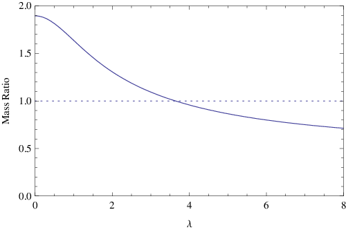
Fig. 1 shows the mass RG flows of the first and the third generation sleptons with and without the hidden sector effects, and Fig. 2 shows similar results for the squarks. The messenger scale is taken to be $M=10^{12}$ GeV. In both Fig. 1 and Fig. 2, we see that the hidden sector renormalization (down to the hidden scale $M_{\rm hid}$) gives rise to smaller soft scalar masses, compared to the flows without it. This effect is readily understood by looking at the RGE (25)-(31), in which the effects of the hidden sector renormalization are the positive terms $4\lambda^{2}m_{i}^{2}$ on the right hand sides¹¹ 1 In GMSB a hidden sector field need be an MSSM gauge singlet and a possible model of hidden sector superpotential is Yukawa type, as (5). Then the hidden sector contributions to RGE are always positive. . It is also obvious from the RGE that larger $\lambda$ gives smaller soft scalar masses at low energy. In contrast, the RGE and hence the low energy mass spectrum of the gauginos are not affected by the hidden sector renormalization. This implies that the lightest scalar superparticle, namely the lightest stau, can be lighter than the lightest gaugino, i.e. bino, for sufficiently large $\lambda$. In Fig. 3, we plot the stau/neutralino mass ratio $m_{\tilde{\tau}}/m_{\tilde{\chi}^{0}}$ at the electroweak scale as a function of $\lambda$ with $M=10^{12}$ GeV. $\lambda=0$ corresponds to no hidden sector RG effects, reproducing the known result of neutralino NLSP in the minimal GMSB scenario. As $\lambda$ is increased²² 2 The perturbative means is valid for $\lambda^{2}/(4\pi)\lesssim 1$. Our choice of the parameter in the following discussions is roughly within this range. , the mass $m_{\tilde{\tau}}$ of the lightest stau $\tilde{\tau}$ becomes smaller, while the neutralino mass $m_{\tilde{\chi}^{0}}$ remains the same; the stau becomes lighter than the neutralino when $\lambda\gtrsim 3.7$. For example, $M=10^{12}$ GeV and $\lambda=3.8$ yields $m_{\tilde{\tau}}=132$ GeV and the neutralino (bino) mass $m_{\tilde{\chi}^{0}}=135$ GeV at the electroweak scale. This stau mass is compatible with the LEP bound for long-lived massive charged particles $\gtrsim$ 102.0 GeV [18].

The ratio of the stau and the bino masses $m_{\tilde{\tau}}/m_{\tilde{\chi}^{0}}$ is depicted in Fig. 4, against the messenger scale $M$ for various values of $\lambda$. The vertical dashed line indicates the minimal messenger scale determined by the condition that gravitino is cold dark matter, $m_{3/2}\gtrsim 0.1$ MeV. Here the gravitino mass is given by [19, 20]

$\displaystyle m_{3/2}\sim{F\over\sqrt{3}M_{P}}={M\over\sqrt{3}M_{P}}\Lambda,$

(19)

where $M_{P}=2.4\times 10^{18}$ GeV is the reduced Planck mass. The gravitino mass is also affected by the hidden sector renormalization [14]. For example, when the source of the supersymmetry breaking is a term linear in $X$, the vacuum expectation value of the $F$-term component of $X$ is proportional to the wave function renormalization factor $Z_{X}^{-1/2}=\exp(-\frac{1}{2}\int_{t}^{0}dt\gamma(t))$. This takes effect from the messenger scale down to the hidden scale, resulting in suppression of the gravitino mass by the factor $Z_{X}^{-1/2}\approx 0.5$ for $\lambda=2\sim 4$. Taking this suppression into account, the minimal messenger scale consistent with the cold dark matter condition $m_{3/2}\gtrsim 0.1$ MeV is $M_{*}\approx 9.0\times 10^{9}$ GeV. By choosing an appropriate messenger scale $M$ within $M_{*}\lesssim M\lesssim 10^{12}$ GeV, stau can be the NLSP with $\lambda$ as small as $3.0$.

In the previous section we have seen that the hidden sector renormalization can change the low energy mass spectrum. Here we describe phenomenological implications when the NLSP is the lightest stau.

We note that cosmological constraints on the mass parameters in the stau NLSP scenario are less stringent than in the neutralino NLSP case [5]. In BBN, stau produces a bound state with ⁴He that tends to overproduce primordial ⁶Li through catalytic reaction ${}^{4}{\rm He}\ \tilde{\tau}^{-}+{\rm D}\rightarrow{}^{6}{\rm Li}+\tilde{\tau}^{-}$ [21, 22] (see also [23, 24, 5]), giving upper bound for the stau lifetime³³ 3 This constraint may be relaxed by considering substantial leftÐright mixing of the stau mass eigenstates [25].

	$\displaystyle\tau_{\tilde{\tau}}$	$\displaystyle=$	$\displaystyle\Gamma^{-1}(\tilde{\tau}\rightarrow\tau\tilde{G})\simeq\frac{48\pi m_{3/2}^{2}M_{P}^{2}}{m_{\tilde{\tau}}^{5}}\left(1-\frac{m_{3/2}^{2}}{m_{\tilde{\tau}}^{2}}\right)^{-4}$		(20)
		$\displaystyle\simeq$	$\displaystyle 5.7\times 10^{4}\left(\frac{m_{3/2}}{1\;{\rm GeV}}\right)^{2}\left(\frac{100\;{\rm GeV}}{m_{\tilde{\tau}}}\right)^{5}$
		$\displaystyle\lesssim$	$\displaystyle 5\times 10^{3}\ {\rm seconds}.$

Fig. 5 shows the stau lifetime $\tau_{\tilde{\tau}}$ plotted against the stau mass $m_{\tilde{\tau}}$ for different values of gravitino mass $m_{3/2}$. The upper bound of the stau lifetime $\tau_{\tilde{\tau}}\lesssim 5\times 10^{3}$ constrains the gravitino mass from above. For our typical range of stau mass $m_{\tilde{\tau}}\approx 130$ GeV, the gravitino mass is $m_{3/2}\lesssim 0.6$ GeV. Together with the condition that gravitino behaves as cold dark matter, a successful cosmological scenario with stau NLSP and gravitino cold dark matter requires the gravitino mass to be within $0.1$ MeV $\lesssim m_{3/2}\lesssim 0.6$ GeV. The model prediction (19) is safely within this range.

The origin of relic gravitino is either thermal or non-thermal productions. The thermal production is due to scattering in the thermal plasma in the radiation dominated era after inflation. The relic abundance from this contribution is computed as [26, 27, 28]

$$\Omega_{\tilde{G}}^{\rm TP}h^{2}\simeq 0.3\left(\frac{T_{R}}{10^{10}{\rm GeV}}\right)\left(\frac{100{\rm GeV}}{m_{3/2}}\right)\left(\frac{M_{3}}{1{\rm TeV}}\right)^{2},$$

(21)

where $T_{R}$ is the reheating temperature and $h$ is the Hubble constant in the unit of 100 km Mpc^-1s^-1. The non-thermal production of gravitino is due to decay of the NLSP ⁴⁴ 4 The productions of gravitino from decay of moduli, inflation, and Polonyi fields have also been discussed [29, 30, 31, 32, 33, 34, 35, 36, 37]. [38, 39]. The abundance of non-thermally produced gravitino is estimated as [40, 41, 42, 43]

$$\Omega_{\tilde{G}}^{\rm NTP}h^{2}=\frac{m_{3/2}}{m_{\tilde{\tau}}}\Omega_{\tilde{\tau}}^{\rm th}h^{2}\simeq 0.02\left(\frac{m_{3/2}}{100{\rm GeV}}\right)\left(\frac{m_{\tilde{\tau}}}{1{\rm TeV}}\right),$$

(22)

where $\Omega_{\tilde{\tau}}^{\rm th}$ is the thermal abundance of stau. The total gravitino abundance is thus

$$\Omega_{\tilde{G}}h^{2}=\Omega_{\tilde{G}}^{\rm TP}h^{2}+\Omega_{\tilde{G}}^{\rm NTP}h^{2},$$

(23)

which is constrained by the observed dark matter density [1]

$$\Omega_{\tilde{G}}h^{2}\leq\Omega_{CDM}h^{2}\simeq 0.1131\pm 0.0034.$$

(24)

For stau mass $m_{\tilde{\tau}}\approx$ 130 GeV, the BBN bound for the gravitino mass $m_{3/2}\lesssim 0.6$ GeV restricts the non-thermally produced gravitino abundance (22) to be extremely small, $\Omega_{\tilde{G}}^{\rm NTP}h^{2}\lesssim 10^{-5}$, indicating that most of the gravitino dark matter is produced thermally. The BBN bound for the gravitino mass and the dark matter abundance (24) gives an upper bound of the reheating temperature. Using (21), we find $T_{R}\lesssim 10^{7}$ GeV. The model prediction (19) with $M=10^{12}$ GeV and $\Lambda=10^{5}$ GeV yields $m_{3/2}\approx 11$ MeV; if the right amount of gravitino dark matter of this mass is to be produced thermally ($\Omega_{CDM}=\Omega_{\tilde{G}}^{\rm TP}$), one needs $T_{R}\approx 10^{6}$ GeV. This is lower than the reheating temperature required for successful leptogenesis; the observed baryon asymmetry needs to be generated by some other mechanism, such as [44].

Stau NLSP is also of interest for collider phenomenology. Eq. (17) implies that the lifetime of stau $\tau_{\tilde{\tau}}$ may be long, depending on the gravitino and stau masses; for instance, $\tau_{\tilde{\tau}}\approx 100$ sec for $m_{\tilde{\tau}}=130$ GeV and $m_{3/2}=0.1$ GeV. For a particle with such a long lifetime, the decay length well exceeds the size of detectors and the decay takes place outside detectors. There have been intriguing proposals for trapping such long-lived charged NLSPs outside detectors [6, 7, 8, 9, 10]. It has been pointed out that detailed studies of stau decay may provide precise measurements of the gravitino mass and the supersymmetry breaking scale. This would also be a crucial test of supergravity since the stau decay $\tilde{\tau}\rightarrow\tau\tilde{G}$ involves supergravity effects.

In this paper we studied the effects of hidden sector renormalization in the minimal GMSB model, using a toy model of the hidden sector field $X$ with self-coupling $\lambda$. We saw that the soft scalar and gravitino masses are affected by the hidden sector RG; they become smaller than the conventional GMSB RG results. Since the gaugino masses are unaltered, the resulting low energy mass spectrum of the superparticles can be quite different from the conventional GMSB. In particular, we find that stau, instead of neutralino, can be the NLSP in the minimal GMSB model. Based on this observation we also discussed phenomenological implications of stau NLSP and gravitino cold dark matter arising from the model. With our typical choice of parameter values: the messenger scale $M=10^{12}$ GeV, $\tan\beta=10$, $\Lambda=F/M=10^{5}$ GeV and the hidden sector coupling $\lambda=3.8$, the model yields stau NLSP with mass $m_{\tilde{\tau}}\approx 130$ GeV. The gravitino mass arising from these parameter values is shown to be consistent with the BBN constraints. It was also shown that gravitino cold dark matter with observationally consistent abundance is attributed to thermal production in this scenario.

We comment that the hidden sector dependence of the mass spectra, as discussed in this paper, does not necessarily mar the predictability of the GMSB scenario. Rather, the hidden sector only influences the soft scalar and the gravitino masses, and the beauty of the GMSB scenario is kept intact. In fact, as emphasized in [12, 13, 14], the effects of the hidden sector RG can be viewed as a new window to look into the hidden sector using the low energy mass spectrum that is expected to be revealed in experiments such as Large Hadron Collider. While the model discussed here represents a simple toy example of many possible hidden sector models, we believe essential features of our results to be generic. For example, only the soft scalar and the gravitino masses, and not the other masses neither the couplings, are subject to the hidden sector RG effects. This is a consequence of the powerful non-renormalization theorem and we do not expect this feature to be dependent on details of the hidden sector. Needless to say, however, there might be various other model-dependent issues that deserve further study.

References

- [1] E. Komatsu et al. (WMAP), Astrophys. J. Suppl. 180, 330 (2009), eprint 0803.0547.
- [2] M. Dine, W. Fischler, and M. Srednicki, Nucl. Phys. B189, 575 (1981); S. Dimopoulos and S. Raby, Nucl. Phys. B192, 353 (1981); L. Alvarez-Gaume, M. Claudson, and M. B. Wise, Nucl. Phys. B207, 96 (1982); M. Dine and W. Fischler, Nucl. Phys. B204, 346 (1982); C. R. Nappi and B. A. Ovrut, Phys. Lett. B113, 175 (1982); M. Dine and A. E. Nelson, Phys. Rev. D48, 1277 (1993), eprint hep-ph/9303230; M. Dine, A. E. Nelson, and Y. Shirman, Phys. Rev. D51, 1362 (1995), eprint hep-ph/9408384; M. Dine, A. E. Nelson, Y. Nir, and Y. Shirman, Phys. Rev. D53, 2658 (1996), eprint hep-ph/9507378.
- [3] S. Dimopoulos, M. Dine, S. Raby, and S. D. Thomas, Phys. Rev. Lett. 76, 3494 (1996), eprint hep-ph/9601367.
- [4] S. Dimopoulos, S. D. Thomas, and J. D. Wells, Nucl. Phys. B488, 39 (1997), eprint hep-ph/9609434.
- [5] M. Kawasaki, K. Kohri, T. Moroi, and A. Yotsuyanagi, Phys. Rev. D78, 065011 (2008), eprint 0804.3745.
- [6] W. Buchmuller, K. Hamaguchi, M. Ratz, and T. Yanagida, Phys. Lett. B588, 90 (2004), eprint hep-ph/0402179.
- [7] J. L. Feng, A. Rajaraman, and F. Takayama, Int. J. Mod. Phys. D13, 2355 (2004), eprint hep-th/0405248.
- [8] K. Hamaguchi, Y. Kuno, T. Nakaya, and M. M. Nojiri, Phys. Rev. D70, 115007 (2004), eprint hep-ph/0409248.
- [9] J. L. Feng and B. T. Smith, Phys. Rev. D71, 015004 (2005), eprint hep-ph/0409278.
- [10] K. Hamaguchi, M. M. Nojiri, and A. de Roeck, JHEP 03, 046 (2007), eprint hep-ph/0612060.
- [11] R. N. Mohapatra, N. Okada, and H.-B. Yu, Phys. Rev. D78, 075011 (2008), eprint 0807.4524.
- [12] M. Dine et al., Phys. Rev. D70, 045023 (2004), eprint hep-ph/0405159.
- [13] A. G. Cohen, T. S. Roy, and M. Schmaltz, JHEP 02, 027 (2007), eprint hep-ph/0612100.
- [14] B. A. Campbell, J. Ellis, and D. W. Maybury (2008), eprint 0810.4877.
- [15] N. Seiberg, Phys. Lett. B318, 469 (1993), eprint hep-ph/9309335.
- [16] K. A. Intriligator, R. G. Leigh, and N. Seiberg, Phys. Rev. D50, 1092 (1994), eprint hep-th/9403198.
- [17] D. J. Castano, E. J. Piard, and P. Ramond, Phys. Rev. D49, 4882 (1994), eprint hep-ph/9308335.
- [18] G. Abbiendi et al. (OPAL), Phys. Lett. B572, 8 (2003), eprint hep-ex/0305031.
- [19] S. Deser and B. Zumino, Phys. Rev. Lett. 38, 1433 (1977).
- [20] E. Cremmer et al., Phys. Lett. B79, 231 (1978).
- [21] M. Pospelov, Phys. Rev. Lett. 98, 231301 (2007), eprint hep-ph/0605215.
- [22] R. H. Cyburt, J. R. Ellis, B. D. Fields, K. A. Olive, and V. C. Spanos, JCAP 0611, 014 (2006), eprint astro-ph/0608562.
- [23] K. Kohri and F. Takayama, Phys. Rev. D76, 063507 (2007), eprint hep-ph/0605243.
- [24] M. Kaplinghat and A. Rajaraman, Phys. Rev. D74, 103004 (2006), eprint astro-ph/0606209.
- [25] M. Ratz, K. Schmidt-Hoberg, and M. W. Winkler, JCAP 0810, 026 (2008), eprint 0808.0829.
- [26] M. Bolz, A. Brandenburg, and W. Buchmuller, Nucl. Phys. B606, 518 (2001), eprint hep-ph/0012052.
- [27] J. Pradler and F. D. Steffen, Phys. Rev. D75, 023509 (2007), eprint hep-ph/0608344.
- [28] F. D. Steffen, JCAP 0609, 001 (2006), eprint hep-ph/0605306.
- [29] M. Hashimoto, K. I. Izawa, M. Yamaguchi, and T. Yanagida, Prog. Theor. Phys. 100, 395 (1998), eprint hep-ph/9804411.
- [30] R. Kallosh, L. Kofman, A. D. Linde, and A. Van Proeyen, Phys. Rev. D61, 103503 (2000), eprint hep-th/9907124.
- [31] G. N. Felder, L. Kofman, and A. D. Linde, Phys. Rev. D60, 103505 (1999), eprint hep-ph/9903350.
- [32] A. L. Maroto and A. Mazumdar, Phys. Rev. Lett. 84, 1655 (2000), eprint hep-ph/9904206.
- [33] G. F. Giudice, I. Tkachev, and A. Riotto, JHEP 08, 009 (1999), eprint hep-ph/9907510.
- [34] M. Dine, W. Fischler, and D. Nemeschansky, Phys. Lett. B136, 169 (1984).
- [35] G. D. Coughlan, R. Holman, P. Ramond, and G. G. Ross, Phys. Lett. B140, 44 (1984).
- [36] I. Joichi and M. Yamaguchi, Phys. Lett. B342, 111 (1995), eprint hep-ph/9409266.
- [37] J. J. Heckman, A. Tavanfar, and C. Vafa (2008), eprint 0812.3155.
- [38] J. L. Feng, A. Rajaraman, and F. Takayama, Phys. Rev. Lett. 91, 011302 (2003a), eprint hep-ph/0302215.
- [39] J. L. Feng, A. Rajaraman, and F. Takayama, Phys. Rev. D68, 063504 (2003b), eprint hep-ph/0306024.
- [40] S. Borgani, A. Masiero, and M. Yamaguchi, Phys. Lett. B386, 189 (1996), eprint hep-ph/9605222.
- [41] T. Asaka, K. Hamaguchi, and K. Suzuki, Phys. Lett. B490, 136 (2000), eprint hep-ph/0005136.
- [42] F. D. Steffen, AIP Conf. Proc. 903, 595 (2007a), eprint hep-ph/0611027.
- [43] F. D. Steffen (2007b), eprint 0711.1240.
- [44] I. Affleck and M. Dine, Nucl. Phys. B249, 361 (1985).