Exact Coupling Coefficient Distribution in the Doorway Mechanism
Abstract
In many–body and other systems, the physics situation often allows one to interpret certain, distinct states by means of a simple picture. In this interpretation, the distinct states are not eigenstates of the full Hamiltonian. Hence, there is an interaction which makes the distinct states act as doorways into background states which are modeled statistically. The crucial quantities are the overlaps between the eigenstates of the full Hamiltonian and the doorway states, that is, the coupling coefficients occuring in the expansion of true eigenstates in the simple model basis. Recently, the distribution of the maximum coupling coefficients was introduced as a new, highly sensitive statistical observable. In the particularly important regime of weak interactions, this distribution is very well approximated by the fidelity distribution, defined as the distribution of the overlap between the doorway states with interaction and without interaction. Using a random matrix model, we calculate the latter distribution exactly for regular and chaotic background states in the cases of preserved and fully broken time–reversal invariance. We also perform numerical simulations and find excellent agreement with our analytical results.
1 Introduction
In open quantum systems, strength function phenomena [1] give structural information about the system itself and about the excitation mechanism. Here, we address statistical features of the doorway mechanism which can be defined as follows: there are one or several somehow “distinct” and “simple” excitations whose amplitudes are spread over many “complicated” states. In a many–body system, collective excitations are often distinct, because all or large groups of particles move in a coherent fashion. As compared to the complexity of the other, non–collective excitations, these states can be interpreted in the framework of a ted in the framework of a simple, typically semiclassical, picture. The distinct states act as “doorways” to the background of the complicated states [1, 2]. Mostly, the statistical features of the latter are chaotic. The strength function has Breit–Wigner shape, largely independent of the statistics of the background states. The width characterizing the Breit–Wigner strength function is referred to as spreading width [1].
The doorway mechanism is found in a rich variety of systems, comprising atoms and molecules [3], as well as atomic clusters, quantum dots and, more generally, mesoscopic systems [4, 5, 6]. Nuclear physics provides particularly beautiful and well–studied examples, such as Isobaric Analog States and multipole Giant Resonances [1, 7, 8, 9, 10].
What is a suitable theoretical interpretation of the Breit–Wigner shape? — Although the simple picture for the distinct excitations captures the main physics, it is important to realize that these states are not eigenstates of the real quantum Hamiltonian. Similarly, the statistical models for the background states do not describe eigenstates either. Thus, if we use the simple picture for the distinct states and the statistical model for the background states as a basis of the Hilbert space, there must be a non–vanishing interacting between these two classes of states. Rediagonaliziation then yields proper eigenstates of the model Hamiltonian. Averaging over the background states, one obtains the local density of states around the energy of the distinct state or states in the simple picture. The local density of states is once more of Lorentzian or Breit–Wigner shape with a spreading width that is — depending on the particular situation — closely related to or identical with the above mentioned spreading width in the strength function. It can be viewed as a measure for the quality of the simple picture describing the distinct states: the smaller the spreading width, the closer is this picture to the physics reality.
The strength of the interacting between the two classes of states uniquely determines the spreading width and, equivalently, the size of the overlap between the distinct state in the simple picture and the true eigenstates of the model Hamiltonian. These overlaps are of course the coupling coefficients when expanding the true eigenstates in the above mentioned basis. Recently, a new statistical observable was introduced: the distribution of the maximum coupling coefficients [11]. The first two moments of this distribution were already studied in Ref. [12], but with assumptions not valid in our context. In Ref [11], however, the full distribution is addressed. Importantly, its shape sensitively depends on the interaction strength. Moreover, it is an especially well–tailored measure to investigate weak interactions.
Here, we present exact results for the distribution of the coupling coefficients to a distinct state in the framework of a random matrix model. In the particularly interesting regime of weak interactions, this distribution coincides with the distribution of the maximum coupling coefficients.
2 Posing the Problem
In Sec. 2.1, we present the random matrix model for the doorway mechanism. We introduce and define the distribution of the maximum coupling coefficient in Sec. 2.2.
2.1 Doorway Mechanism in a Random Matrix Model
The model to be discussed here stems from nuclear physics [1] and is also often used in other fields [13]. For the convenience of the reader and to define our notation, we compile its salient features. As we are aiming at a random matrix model, it is convenient to choose from the beginning a proper basis of the full Hilbert space such that we can represent the Hilbert space operators by matrices. Introducing a cutoff, their dimension is finite. Eventually this cutoff effect is removed by taking the matrix dimension to infinity. We nevertheless use the Dirac notation for the wave functions, even though they are finite–dimensional vectors.
The total Hamiltonian consists of three parts, the Hamiltonian for the distinct states which become the doorway states, the Hamiltonian describing the background states, where will eventually be taken to infinity, and the interaction coupling the two classes of states. Hence, we have
| (1) | |||||
For the matrix elements of the interaction, we make the assumptions and for any , , , . Often, there is only one relevant doorway state or the spacing between the doorway states is much larger than their spreading widths. We focus on these cases and consider only one doorway state by setting , and .
The eigenequations for the uncoupled Hamiltonians are
| (2) |
Due to the interaction the doorway state is not an eigenstate of the Hamiltonian . We denote the eigenstates of the full Hamiltonian by . The eigenequation to be solved is
| (3) |
Resembling the situation in most systems, we put the doorway state in the center of the background spectrum. It interacts with the surrounding states. Without loss of generality, we may set .
The exact eigenstate of which evolves from the doorway state in the presence of the interaction is referred to as . We expand the –th eigenstate of in the basis spanned by and as
| (4) |
where the coupling coefficient is the overlap between the doorway state in the non–exact picture for this distinct state and the –th exact eigenstate of the full Hamiltonian. We are interested in the statistical features of these coupling coefficients.
We have to solve our model for . The action of the full Hamiltonian on the eigenstate yields on the one hand
| (5) |
On the other hand we have
| (6) |
Equating these two expressions, we find
| (7) |
such that
| (8) |
Using the normalization of , we eventually arrive at
| (9) |
which is the desired expression for in terms of the matrix elements of .
Formula (9) holds for . This expression is still exact. However, since the eigenvalues of the full Hamiltonian depend on the coupling coefficents , it is a complicated implicit expression. We proceed further by expanding the exact eigenvalues perturbatively in ,
| (10) |
where the eigenstate of the full Hamiltonian to eigenvalue has evolved from the eigenstate of the unperturbed Hamiltonian by adiabatically switching on the perturbation.
We now obtain a crucial simplification by setting , i. e. we keep only the leading order term in the perturbative expansion of Eq. (10). To this approximation of for the sum in Eq. (9) is completely dominated by the term , which actually diverges such that to first order for all . The only overlap integral which remains finite is the overlap of the doorway state with itself . Here we set and no divergence occurs. Using the approximation we have therefore essentially singled out as the only non–vanishing – and thus inevitably maximum – overlap integral of the perturbed eigenstates with the doorway state.
2.2 Distribution of the Maximum Coupling Coefficient
The new statistical observable introduced in Ref. [11] is the distribution of the maximum
| (11) |
of the overlaps between the eigenstates of the full Hamiltonian and the distinct state, that is the doorway state . In order to obtain it, we have to average in a suitable way over the interaction matrix elements and over the Hamiltonian modeling the background states. For the time being it suffices to denote this average by square brackets. Later on we give a precise definition. Hence, the distribution in question is given by
| (12) |
On the other hand, the distribution of overlap between the evolved doorway state and the unperturbed doorway state reads
| (13) |
Setting amounts essentially to the approximation
| (14) |
This approximation is certainly good for small interactions or, more precisely, as long as the mean coupling strength is an order of magnitude smaller than the mean level density of the background states. Our numerical simulations will strongly corroborate this statement. Hence, we focus on , which can be treated analytically.
The statistics of the interaction matrix elements can only have minor impact on the resulting distribution. Hence, if not stated otherwise assume that the interaction matrix elements are Gaussian distributed random variables. We have to distinguish two cases. The total Hamiltonian can be time–reversal non–invariant or time–reversal invariant, where we disregard spin degrees of freedom. In the first case, labeled by the Dyson index , the interaction matrix elements are complex variables, in the second case, labeled , they are real. Introducing the –component vector , the corresponding distribution is
| (15) |
In addition to the behavior under time–reversal invariance, the statistical properties of the Hamiltonian , however, must strongly affect the distribution . Hence, we do not specify it yet. As is well known from Random Matrix Theory, the parameter governing the physics is
| (16) |
where is the mean level spacing of the background states in the center of the band [1, 13]. The distribution is chosen such that is independent of .
Technically, it is more convenient to work out the probability density of the random variable
| (17) |
The relation between the two distributions reads
| (18) |
Thus, once is known, follows immediately.
We now use our statistical assumption that the interaction matrix elements are Gaussian distributed. We write the distribution in the form
| (19) |
where is the product of the differentials of all independent variables in . The square brackets with index denote an average over the background states, that is, over the Hamiltonian . For the calculation of the averages, it is helpful to write the distribution as the Fourier transform
| (20) |
with the characteristic function
| (21) |
After rescaling we obtain the alternative expression
| (22) | |||||
where the vector has real entries for and complex ones for , respectively. The infinitesimal volume element is a product of the differentials of all independent entries of the vector . As a generating function is normalized to .
In the sequel, we calculate the expressions (22) for generic choices of the Hamiltonian governing the dynamics of the background states.
3 Regular Background
The doorway state is embedded into a regular background, if the eigenvalues of do not repel each other. The distribution of the background Hamiltonian then factorizes according to
| (23) |
In order to keep the discussion most general we use for the interaction matrix elements a general factorizing distribution
| (24) |
instead of the Gaussian distribution introduced before Eq. (15). We keep the reasonable, physically motivated assumption of statistical independence of the interaction matrix elements but relax the global orthogonal () or unitary () invariance of the interaction matrix elements, implicit in the measure Eq. (15). For complex coupling matrix elements we assume in addition that the distribution is invariant . We asign to complex coupling matrix elements with this invariance the Dyson index and to real coupling matrix elements the Dyson index .
A straightforward calculation reveals that the characteristic function (21) factorizes as well and becomes an –th power of a single integral,
| (25) | |||||
| (26) |
As we are interested in the local scale set by the mean level spacing of the background states, the distribution should not be sensitive to the particular choice of the distribution , as long as it does not contain scales competing with the mean level spacing . The simplest choice is
| (27) |
where and is the length of the background spectrum. The following calculation is similar to the one described in the Appendix B of Ref. [14]. We perform the integral over the background distribution in Eq. (26)
| (28) | |||||
In the last equation we used an integral identity of the Fresnel type
| (29) |
We find for the characteristic function
| (30) | |||||
| (31) |
We observe that the distribution of the interaction matrix elements enters only via the expectation value as defined in Eq. (30) and not via the second moment . As pointed out after Eq. (16) is chosen such that the mean coupling strength, as defined through , is independent of . This means that in general is different for real and for complex coupling. We write , where now depends on Dyson’s index and on the distribution . For instance for the Gaussian distribution we find
| (32) |
Using the definition of in Eq. (16) we finally find
| (33) |
The reader can easily convince herself/himself that other reasonable choices for such as a Gaussian distribution yield the same functional form as in Eq. (33). The Fourier transform (20) results in
| (34) |
Using the relation (18), we eventually arrive at
| (35) |
As anticipated, the interaction strenght enters the distribution only via the dimensionless ratio . The distribution enters via the the factor defined in Eq. (30). It is interesting to see that does not only depend on the distribution but also on the symmetry factor . This means that for a regular background and for constant interaction strength the distribution distinguishes between real interaction and complex interaction. As we will see in the following this does not happen for a chaotic background. Therefore here opens – at least theoretically – the possiblity to distinguish between a regular and a chaotic background dynamics through the doorway state.
Assume we can experimentally manipulate the interaction between the Doorway state and the background such the interaction matrix elements change from real to complex, for instance by switching on a magnetic field. For fixed mean interaction strength and for a chaotic background dynamics the distribution will be invariant, whereas for a regular background it will change.

In Fig. 1 is plotted for three different values of the mean coupling strength. We see that due to the numerical similarity of and the plots for real and for complex couplings are almost the same. The fact that for a Gaussian distribution seems to be rather accidental. However for being a semicircle (SC) distribution we find and and for a uniform (U) distribution we find and . In other words, for physically reasonable distribution functions we have , which encumbers the experimental possibility sketched above.
4 Chaotic Background
The dynamics of the background states is usually chaotic. The Hamilton matrix modeling the background states has then to be chosen from a Gaussian random matrix ensemble. Again, we have to distinguish time–reversal invariant and non–invariant systems, that is, the cases labeled by the Dyson parameters and , respectively. The Hamiltonian is from the Gaussian orthogonal ensemble (GOE) for and from the Gaussian unitary ensemble (GUE) for with variance of the diagonal elements
| (36) |
As already said, is an –component vector which has real or complex entries for and , respectively.
In Sec. 4.1 we reformulate the problem in terms of matrix invariants. This enables us to introduce a handy supermatrix model in Sec. 4.2, which we then solve in Sec. 4.3.
4.1 Reformulation in a Rotation–Invariant Form
At first sight, the best way of tackling the problem seems to start from Eq. (19) and to introduce . The integration is then simply an integration over a sphere in a real or complex space. This leads to
| (37) |
where the matrix
| (38) |
has rank one. Furthermore,
| (39) |
is the volume of the above mentioned sphere. Unfortunately, the remaining ensemble average is only feasible for the GUE, we carry it out in A. For the GOE, the calculation is hampered by the modulus of the determinant.
To adress the GOE case and to have a method that is capable of handling both cases, GOE and GUE, in a unifying way, it turns out necessary to cast the ensemble average into an invariant form. To this end, we start from Eq. (22), perform the integration over the vector and obtain
| (40) |
Now we make the observation, that the –matrix average can be expressed as an –matrix average as follows
| (41) |
where is a matrix and the ensemble average is over an –matrix GOE (GUE) ensemble. The derivation of Eq. (41), which is crucial for the calculation, is sketched in App. B. On the right hand side, the inconvenient modulus of the determinant has disappeared. The combinatorial factor is given by
| (42) |
We express the determinant on the right hand side of Eq. (41) as a Gaussian integral over a real () or complex () vector .
| (43) |
and plug subsequently Eqs. (40), (41) and (43) into Eq. (20) and write the integral over the vector in radial coordinates. We find
| (44) | |||||
where we introduced the function
| (45) |
with the matrix .
After combining the various constants we arrive at
| (46) | |||||
where we introduced formally the fractional derivative
| (47) |
We can evaluate the fractional distribution
| (48) | |||||
for arbitrary . For we obtain
Here we see that the GOE case is more complicated than the GUE case.
For the GUE the fractional derivative disappears and we find without further problems
| (52) |
For the GOE we obtain an integral expression
| (53) |
The remaining task is in both cases (GOE and GUE) the calculation of .
4.2 Mapping onto a Supermatrix Model
Using
| (54) | |||||
the ensemble average defined in Eq. (45) can be expressed via standard techniques as a supersymmetric matrix integral
| (55) | |||||
Here and are (GUE) respectively (GOE) supermatrices of the form
The matrix entries in latin letters denote real commuting integration variables. The matrix entries in greek letters denote complex anticommuting integration variables. The infinitesimal volume elements and are products of the differentials of all independent integration variables. The integration domain of the real commuting variables is the real axis. The matrix is a (GUE) or a (GOE) diagonal supermatrix with entries (GUE) and (GOE). Due to the broken rotation invariance of the original matrix model (1) the resulting supersymmetric representation (55) is a two–matrix model.
We wish to evaluate the –integral by a saddle–point approximation and to calculate the integral exactly afterwards. It is well known [15] that the integral yields for large in the saddle–point approximation
| (64) | |||||
where is the mean level spacing in the center of the band. However this approximation is only valid, if itself is of order of the mean level spacing. Since the integration domain of is the whole real axis, this is not automatically guaranteed. A necessary condition is that the variance of the Gaussian in the second line of Eq. (55) is itself of order of the mean level spacing, i. e. the integral in Eq. (55) is essentially localised to a small window of width around zero. Consequently we must require
| (65) |
And therefore should scale as for large . The dimensionless coupling strength is given by . Since it is of order one, we obtain for in the GUE case
| (66) | |||||
Fortunately this is exactly the scaling behaviour we need to apply the saddle–point approximation. In the GOE case Eq. (66) holds in any Intervall , where is an infrared cutoff in the integral, which is small compared to one but large compared to the mean level spacing. i.e. in the limit in the whole integration domain of the –integral in Eq. (53). In conclusion we can apply the approximation (64) both in the GUE as well as in the GOE case.
4.3 Remaining Matrix Integration and Final Result
Plugging Eq. (64) into Eq. (55) we obtain after a simple shift
| (67) |
where we also employed that . Now the derivative with respect to the source term can be performed
| (68) | |||||
where we used the identity
| (69) |
for a complex number with negative imaginary part. The remaining average can be calculated by employing techniques of standard analysis. We use
| (70) |
which holds for . We obtain
| (71) |
Finally we obtain
| (72) | |||||
This result simplifies considerable when we take into account the scaling behavior (66) of . In the large limit we can write
| (73) |
This can now be plugged into Eq. (46) to obtain expressions for on the scale of the mean level spacing. For the GUE we find straightforwardly
| (74) |
For the GOE we are left with an integral expression for
| (75) |
The integral can be evaluated further and be expressed in terms of standard special functions. Finally we arrive at
| (76) | |||||
where is the modified Bessel function of the second kind of order .

4.4 Comparison
In Fig. 3 the distribution function of the overlap integral of the evolved doorway state with the unperturbed doorway state is plotted for four different coupling strengths , , and and for all types of couplings and background complexities considered. These are: 1) complex coupling to a regular background (dashed blue line), 2) real coupling to a regular background (full blue line), 3) complex coupling to a GUE background (full red line) and 4) real coupling to a GOE background (full green line). As a general trend mixing with the background is strongest for a complex coupling to a GUE background and weakest for real coupling to Poissonian background. However the difference of the distributions for different background complexities is rather small. This suggests a certain degree of universality of the curves. One might choose other ensembles for the background Hamiltonian, as for instance semi–Poisson[16] or transition ensembles. However we expect that for these ensembles which lie between the two extreme cases, GUE and Poissonian, their corresponding distributions will also lie in the channel between the full red line (GUE) and the full blue line (Poissonian with real coupling). For the most interesting case of small this channel is small.
On the other hand the distributions are highly sensitive with respect to a change in the coupling strength .

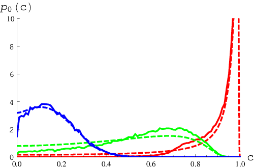
In Fig. 4 we compare the curves for obtained from the analytical results (in this case from Eq. (76)) with Monte Carlo simulations in the case of a real coupling to a GOE background. The figure shows for three values of the coupling strength , and . We see fairly good agreement for all three values, even for the strong coupling value . This shows that the approximation implied in Eq. (10) and thereafter, is justified far beyond the perturbative regime.
5 Discussion
The distribution of the maximum coupling coefficients in the doorway mechanism has been introduced as a new statistical observable. These coupling coefficients, that is, the overlaps between the eigenstates of the full Hamiltonian and the doorway state are not always at the disposal. However, in situations where they are accessible, this distribution provides a highly sensitive measure for the interaction strength. Of particular interest is the regime of weak interactions. In this regime, the distribution of the maximum coupling coefficients is very well approximated by the distribution of the overlap between the evolved doorway state and the unperturbed doorway state. While calculating the former seems unfeasible at present, we calculated the latter exactly for regular and chaotic background states in the cases of preserved and fully broken time–reversal invariance. We performed our calculations in the framework of Random Matrix Theory which is well–known to provide reliable models for regular and chaotic systems. We also carried out numerical simulations which fully confirm our analytical results.
Our exact calculations are of general interest for matrix models. We managed to reformulate a problem with breaking of rotation invariance in the space of random matrices in terms of a rotation invariant problem involving random matrices. This made it possible to map the matrix model in ordinary space onto a matrix model in superspace, which we solved by a saddle point approximation in the limit of infinite level number. Remarkably, the supermatrix model is in the class of two–matrix models which show up in a large variety of situations.
Appendix A GUE Background with Finite Level Number
We define the average
| (77) |
where the diagonal matrix is defined as . Her is related to the parameter of the main text as . The integration is over the set of all Hermitean matrices, i. e. over the GUE ensemble. The normalisation is chosen such that . The task is to calculate the average
| (78) |
A Laplace expansion of the determinant yields
| (79) |
where is the permutation group. Obviously only terms contribute.
| (80) |
It is useful to expand the remaining sum in cycles involving the index . For indices and we define the cycles as
| (81) |
Since the indices do not appear in the remainder of the product, we can integrate over the remainder separately. This yields
| (82) |
The average over the cycles is simple as well. Only terms involving the index yield a factor different from . We ontain
| (83) |
The averages are independent of the indices . The sum over the indices yields the combinatorial factor . Altogether we obtain
| (84) | |||||
Evaluating this equation for allows us to replace the sum. After some further simple manipulations we finally obtain
| (85) |
which is almost our final result. The remaining task is to evaluate the independent constant . This is facilitated by the observation that
| (86) |
where is the standard GUE kernel as defined in Eq. (6.2.10) of Metha’s book (third edition). The
| (87) |
are oscillator wave functions and is the –th Hermite polynomial. The constant can also be evaluated
| (88) |
Of course is but the inverse level spacing at the center of the semicircle. Therefore . We obtain our final result
| (89) |
where
| (90) |
The even–odd difference disappears in the large limit. In the following we set . Using Eq. (37) we find for
| (91) | |||||
This exact result can be compared with Eq. (52) in order to find a differential equation for
| (92) | |||||
This differential equation can easily be solved. However the solution
| (93) | |||||
is highly complicated. It discourages any attempt to calculate the matrix integral Eq. (55) for finite in the GOE case. To make contact with the results obtained in the main text, we introduce the function
| (94) |
With a change of variables in the integral we can write
| (95) |
which coincides with Eq. (72) in the large limit and for .
Appendix B Derivation of Eq. (41)
We define the function
| (96) |
where is a GOE or GUE random matrix and the brackets denote the corresponding GOE or GUE average. is an analytic function in the cut complex plane . In this Appendix we prove the identity
| (97) |
where is a GOE or GUE random matrix. The constant is given in Eq. (42). We write the rhs of Eq. (97) in angle eigenvalue coordinates , where is a diagonal matrix of the eigenvalues of . Since the average is over an invariant function the integral over the diagonalizing group is trivial. The average on the rhs. can now be written as
| (98) | |||||
The power of the Vandermode determinant arises as Jacobian from the coordinate transformation. The constant arising from the group integration can be found in Mehta’s book [17]. Now the integral over the –distribution can be performed.
| (99) | |||||
We see that the resulting integral can be written as a GOE (GUE) average over matrices. This is indicated by using instead of as integration variables. We go back to Cartesean coordinates and find
| (100) | |||||
This is the desired identity with . Eq. (41) is obtained for .
References
References
- [1] Bohr A and Mottelson B 1969 Nuclear Structure Vol. 1 9th ed (New York: W. A. Benjamin)
- [2] Sokolov V V and Zelevinsky V 1997 Phys. Rev. C 56 311
- [3] Herzberg G and Brügel W 1973 The spectra and structures of free simple radicals 1st ed (Darmstadt: D. Steinkopff)
- [4] Guhr T and Weidenmüller H A 1990 Chem. Phys. 146 21
- [5] Kawata I, Kono H, Fujimura Y and Bandrauk A D 2000 Phys. Rev. A 62 031401(R)
- [6] Hussein M S, Kharchenko V, Canto L F and Donangelo R 2000 Ann. Phys. 284 178
- [7] Harney H L, Richter A and Weidenmüller H A 1986 Rev. Mod. Phys. 58 607
- [8] Zelevinsky V 1996 Ann. Rev. Nucl. Part. Sci. 45 237
- [9] Åberg S, Heine A, Mitchell G and Richter A 2004 Phys. Lett. B 598 42
- [10] Shevchenko A, Carter J, Fearick R W, Förtsch S V, Fujita H, Fujita Y, Kalmykov Y, Lacroix D, Lawrie J J, von Neumann-Cosel P, Neveling R, Ponomarev V Y, Richter A, Sideras-Haddad E, Smit F D and Wambach J 2004 Phys. Rev. Lett. 93 122501
- [11] Åberg S, Guhr T, Miski-Oglu M and Richter A 2008 Phys. Rev. Lett. 100 204101
- [12] Vergini J J M 2004 J. Phys. A 37 6507
- [13] Guhr T, Müller-Gröling A and Weidenmüller H A 1998 Phys. Rep 299 189
- [14] Mello P A 1995 Mesoscopic Quantum Physics (Amsterdam: Elsevier)
- [15] Verbaarschot J J M and Zirnbauer M 1985 J. Phys. A 17 1093
- [16] Bogomolny E et al. 2006 Phys. Rev. Lett. 97 254102
- [17] Mehta M L 2004 Random Matrices 3rd ed (Amsterdam: Elsevier)