跳到论文正文
W Papers独立论文阅读器 arXiv:1001.1389 论文正文 计算阅读时间 · 0%
引用这篇论文根据当前论文元数据生成,正式投稿前建议核对。


License: arXiv.org perpetual non-exclusive license
arXiv:1001.1389v1 [cs.IT] 09 Jan 2010

Optimal Cooperative Relaying Schemes for Improving Wireless Physical Layer Security

Jiangyuan Li, Athina P. Petropulu, and Steven Weber Affiliation:  Affiliation: Department of Electrical and Computer Engineering
Drexel University, Philadelphia, PA 19104
Abstract
11 1 This work has been supported by NSF under Grant CNS-0905425. Parts of this work were reported in [1], [2].

We consider a cooperative wireless network in the presence of one of more eavesdroppers, and exploit node cooperation for achieving physical (PHY) layer based security. Two different cooperation schemes are considered. In the first scheme, cooperating nodes retransmit a weighted version of the source signal in a decode-and-forward (DF) fashion. In the second scheme, while the source is transmitting, cooperating nodes transmit weighted noise to confound the eavesdropper (cooperative jamming (CJ)). We investigate two objectives, i.e., maximization of achievable secrecy rate subject to a total power constraint, and minimization of total power transmit power under a secrecy rate constraint. For the first design objective with a single eavesdropper we obtain expressions for optimal weights under the DF protocol in closed form, and give an algorithm that converges to the optimal solution for the CJ scheme; while for multiple eavesdroppers we give an algorithm for the solution using the DF protocol that is guaranteed to converge to the optimal solution for two eavesdroppers. For the second design objective, existing works introduced additional constraints in order to reduce the degree of difficulty, thus resulting in suboptimal solutions. In this work, either a closed form solution is obtained, or algorithms to search for the solution are proposed. Numerical results are presented to illustrate the proposed schemes and demonstrate the advantages of cooperation as compared to direct transmission.

Index Terms: 
Secrecy rate, node cooperation, physical layer based security, semi-definite programming.

I Introduction

Privacy and security issues play an important role in wireless networks. Although security is typically addressed via cryptographic approaches, there have been several attempts at addressing security at the physical layer, following the pioneering work of [8]. Recently wireless physical (PHY) layer based security from a information-theoretic point of view has received considerable attention, e.g., [3]-[7]. The wiretap channel, first introduced and studied by Wyner [8], is the most basic physical layer model that captures the problem of communication security. Wyner showed that when an eavesdropper’s channel is a degraded version of the main channel, the source and destination can achieve a positive perfect information rate (secrecy rate). The maximal secrecy rate from the source to the destination is defined as the secrecy capacity and for the degraded wiretap channel is given as the difference between the rate at the legitimate receiver and the rate at the eavesdropper. The Gaussian wiretap channel, in which the outputs at the legitimate receiver and at the eavesdropper are corrupted by additive white Gaussian noise (AWGN), was studied in [9]. Along the same lines, the Gaussian MIMO wiretap channel was investigated and the secrecy capacity of the MIMO wiretap channel was established in terms of an optimization problem over all possible input covariance matrices [10], [13]. There have also been some recent works focusing on secrecy rates based on partial CSI or channel statistics [3, 4, 15]. In [15], the authors derived the ergodic secrecy capacity of Gaussian MIMO wiretap channel and showed that a circularly symmetric Gaussian input is optimal.

The secrecy rate is affected by channel conditions between the source and the destination and also channel conditions between the source and the eavesdroppers. A low cost approach to increase the achievable secrecy rate by exploiting/mitigating channel effects is node cooperation via relays [16]-[21]. A two-stage cooperative approach was recently proposed in [22, 23], and their extended version [24]. In [24], the source first transmits locally to a set of trusted relays, and subsequently, the relays retransmit a weighted version of the signal that they heard (amplify-and-forward (AF)), or a weighted version of the decoded signal (decode-and-forward (DF)). Alternatively, the relays can transmit weighted noise to confound the eavesdropper while the source is transmitting (cooperative jamming (CJ)). In all cases, the objective is to select the weights so as to maximize the secrecy rate under total power constraints, or to minimize the total power under a secrecy rate constraint. The results in [22]-[24] contain sub-optimal weights for both a single eavesdropper and multiple eavesdroppers, due to the difficulty of solving the associated optimization problems. In particular, several criteria for sub-optimal weight design were proposed such as completely nulling out the message signal at all eavesdroppers for DF and AF, and completely nulling out the jamming signal at the destination for CJ. These sub-optimal weights may yield a reduction in the achievable secrecy rate or minimization of total power.

In this paper, we consider the same scenario and problem as in [22]-[24], but focus on obtaining the optimal solution for the DF and CJ schemes. Obtaining the solution for the AF scheme is a more difficult problem and will be addressed in future work. Exploiting certain properties of the objective functions and the constraints, enables us to either obtain closed form solutions, or, if a closed form solution is not possible, propose algorithms to search for the solution.

The remainder of this paper is organized as follows. The mathematical model is introduced in §II. In §III we derive the optimal relay weights that maximize the achievable secrecy rate subject to a total power constraint in the presence of a single eavesdropper for the DF and CJ protocols, and multiple eavesdroppers for DF protocol. In §IV we study the optimal weights that minimize the total power under a secrecy rate constraint for the DF and CJ protocols. Numerical results in §V are presented to illustrate the proposed solutions. Finally, §VI provides some concluding remarks.

I-A Discussion of related work

Our work falls under the general scenario where the source-destination communication is aided by a relay or a helper. Relevant results include the work of [16], where multiple users communicate with a common receiver in the presence of an eavesdropper, and the transmit power allocation policy is determined that maximizes the secrecy sum-rate. In [17], a source, destination, eavesdropper and relay model is considered, in which the relay transmits a noise signal in order to jam the eavesdropper. The rate-equivocation region is derived to show gains and applicable scenarios for cooperation, with the equivocation denoting the uncertainty of the eavesdropper about the source message.

A generalization of [16] and [17] was proposed in [18], in which the helper transmits signals from another source encoder. In [19], inner and outer bounds on the rate-equivocation region were derived for the four-node model for both discrete memoryless and Gaussian channels. In [21], the secrecy rate of orthogonal relay and eavesdropper channels was studied.

Our work in this paper is different from the aforementioned works in the sense that we address the more general case of multiple relays and multiple eavesdroppers. Also, existing works primarily focus on rate-achieving relaying strategies. In our work, we consider pre-defined cooperative schemes without claiming that those schemes are optimal, and determine relay weight and power allocation design that optimize the achievable secrecy rate subject to a power constraint, or minimize the transmit power subject to a secrecy rate constraint.

I-B Notation

Upper case and lower case bold symbols denote matrices and vectors, respectively. Superscripts ∗\ast, TT and †\dagger denote respectively conjugate, transposition and conjugate transposition. Tr⁡(𝐀)\mathrm{Tr}({\mathbf{A}}) denotes the trace of matrix 𝐀\mathbf{A}. 𝐀⪰0{\mathbf{A}}\succeq 0 means that 𝐀{\mathbf{A}} is a Hermitian positive semi-definite matrix. rank⁡(𝐀)\mathrm{rank}({\bf A}) denotes the rank of matrix 𝐀{\bf A}. ‖𝐚‖\|{\bf a}\| denotes Euclidean norm of vector 𝐚{\bf a}. 𝐈n{\bf I}_{n} denotes the identity matrix of order nn (the subscript is dropped when the dimension is obvious). f′​(x)f^{\prime}(x) and f′′​(x)f^{\prime\prime}(x) denote first- and second- order derivatives of f⁡(x)f(x), respectively.

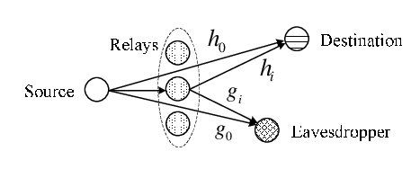
Refer to caption
Fig. 1: System model: source SS wishes to communicate to destination DD in the presence of JJ eavesdroppers, E1,…,EJE_{1},\ldots,E_{J}. The NN relays, R1,…,RNR_{1},\ldots,R_{N} implement decode and forward (DF) or cooperative jamming (CJ), based protocols. In each case the objective is to select the relay weights (𝐰{\bf w}) and the source power (PsP_{s}) to maximize the achievable secrecy rate subject to a total power constraint (P0P_{0}), or to minimize the total power constraint under a secrecy rate constraint.

II System Model and Problem Statement

We consider a wireless network model depicted in Fig. 1, consisting of one source node SS, a set of NN relay nodes (Ri,i=1,…,N)(R_{i},~i=1,\ldots,N), a destination node DD, and a set of JJ passive eavesdroppers (Ej,j=1,…,J)(E_{j},~j=1,\ldots,J). The symbols used in the paper are listed in Table I.

TABLE I: Mathematical notation
NN number of relays
JJ number of eavesdroppers
P0P_{0} total power (source power plus the relays’ power)
PsP_{s} transmit power at the source
σ2\sigma^{2} noise variance
h0h_{0} baseband complex channel gain between the source and the destination
hih_{i} baseband complex channel gain between the iith relay and the destination
aia_{i} baseband complex channel gain between the source and the iith relay
g0​jg_{0j} baseband complex channel gain between the source and the jjth eavesdropper
gi​jg_{ij} baseband complex channel gain between the iith relay and the jjth eavesdropper
𝐰{\bf w} weight vector at the relays, [w1,⋯,wN]T[w_{1},\cdots,w_{N}]^{T}
𝐡{\bf h} [h1,⋯,hN]T[h_{1},\cdots,h_{N}]^{T}
𝐠j\mathbf{g}_{j} [g1​j,⋯,gN​j]T[g_{1j},\cdots,g_{Nj}]^{T}
𝐑h{\bf R}_{h} 𝐡𝐡†{\bf h}{\bf h}^{\dagger}
𝐑gj{\bf R}_{g}^{j} 𝐠j​𝐠j†\mathbf{g}_{j}\mathbf{g}_{j}^{\dagger}
Notes: The index jj is dropped when J=1J=1.

The source message is uniformly distributed over the message set 𝒲={1,2,…,2n​R}\mathcal{W}=\{1,2,...,2^{nR}\}, which is transmitted in nn channel uses. Here, RR denotes the source rate (unit: bits per channel use) and the message has entropy n​RnR bits. A stochastic encoder at the source maps each message to a codeword from an alphabet of length-nn. For the purpose of evaluating the achievable secrecy rate, we assume that the codewords used at the source are Gaussian. We consider a time division multiple access system, in which there are nn time units in each transmission slot. In a time unit, the average power of an encoded source symbol is normalized to unity. The noise at any node is assumed to be zero-mean white complex Gaussian with variance σ2\sigma^{2}. Each node is equipped with a single omni-directional antenna and operates in a half-duplex mode.

All channels are assumed to be flat fading. We assume that global channel state information (CSI) is available, including the eavesdroppers’ channels. This corresponds to the cases where the eavesdroppers are active in the network and their transmissions can be monitored [25]. We should note that there have been some recent works focusing on secrecy rates based on partial CSI or channel statistics (e.g., chapter 5 in [7], and [4]). Adapting the proposed work to cooperative schemes that uses partial CSI or channel statistics will be considered in future work.

Similarly as in [20], [24], we assume that the source encoding scheme, the decoding methods at destination and eavesdroppers, and the cooperative protocol, are all public information.

Let us fix the relay weight vector 𝐰{\bf w} and the source transmission power PsP_{s}. Then the following expressions give the rates with the destination and the eavesdroppers as a function of 𝐰{\bf w}, PsP_{s}, the noise σ2\sigma^{2}, and the various channel gains. For the DF-based protocol, the rate at the destination and the jjth eavesdropper are, respectively

Rd\displaystyle R_{d} =12​log⁡(1+Ps​|h0|2+𝐰†​𝐑h​𝐰σ2),\displaystyle=\frac{1}{2}\log\left(1+\frac{P_{s}|h_{0}|^{2}+{\bf w}^{\dagger}{\bf R}_{h}{\bf w}}{\sigma^{2}}\right), (1)
Rej\displaystyle R_{e}^{j} =12​log⁡(1+Ps​|g0​j|2+𝐰†​𝐑gj​𝐰σ2)\displaystyle=\frac{1}{2}\log\left(1+\frac{P_{s}|g_{0j}|^{2}+{\bf w}^{\dagger}{\bf R}_{g}^{j}{\bf w}}{\sigma^{2}}\right) (2)

where the scalar factor 1/21/2 is due to the fact that two time units are required in two stages. Here we have assumed an additional constraint, i.e., Ps≥P0minP_{s}\geq P_{0}^{\min} where P0minP_{0}^{\min} is the minimum source power requirement for cooperative nodes to correctly decode the source message with high probability. We assume P0minP_{0}^{\min} is known a priori. For the CJ-based protocol, the rate at the destination and the jjth eavesdropper are, respectively

Rd\displaystyle R_{d} =log⁡(1+Ps​|h0|2𝐰†​𝐑h​𝐰+σ2),\displaystyle=\log\left(1+\frac{P_{s}|h_{0}|^{2}}{{\bf w}^{\dagger}{\bf R}_{h}{\bf w}+\sigma^{2}}\right), (3)
Rej\displaystyle R_{e}^{j} =log⁡(1+Ps​|g0​j|2𝐰†​𝐑gj​𝐰+σ2).\displaystyle=\log\left(1+\frac{P_{s}|g_{0j}|^{2}}{{\bf w}^{\dagger}{\bf R}_{g}^{j}{\bf w}+\sigma^{2}}\right). (4)

For both the DF and CJ protocols, the achievable secrecy rate in the presence of JJ eavesdroppers is given by [26]

Rs=max⁡{0,Rd−max1≤j≤J⁡Rej}.R_{s}=\max\{0,R_{d}-\max_{1\leq j\leq J}R_{e}^{j}\}. (5)

In particular, when J=1J=1, i.e., a single eavesdropper, the secrecy rate in (5) becomes [13, 14]

Rs=max⁡{0,Rd−Re}.R_{s}=\max\{0,R_{d}-R_{e}\}. (6)

We consider the practical case in which the system can be designed so that the secrecy rate is positive. In that case, the achievable secrecy rate can be rewritten as

Rs=Rd−max1≤j≤J⁡Rej.R_{s}=R_{d}-\max_{1\leq j\leq J}R_{e}^{j}. (7)

Achievability of the above rates can be shown based on existing results for MIMO wire-tap channels, such as [11], [14], [12], for one eavesdropper, and [26] for multiple eavesdroppers.

The CJ scheme can be viewed as a 1×21\times 2 SIMO system, so that MIMO results are directly applicable. As discussed in [24], for the DF scheme, MIMO results are applicable if we assume that the received signal at destination/eavesdropper at time ii depends only on the relays’ transmitted encoded signals at time ii (though a relay’s transmitted signal at time ii depends on its received signal before time ii). This is usually referred to as the “memoryless relay channel” [17], [19]. For convenience, as in [24] we focus on case in which the relays use the same codewords as the source to re-encode the signal before transmission; in that case the rates of source-destination and source-eavesdropper links admit simple closed-form expressions [24].

The problems addressed in this paper are described as follows.

Problem 1 (maximize secrecy rate under power constraint using DF)

Given total power (source plus relays) P0P_{0}, select source power PsP_{s} and cooperative nodes’ weights 𝐰{\bf w} to maximize the secrecy rate

maxPs,𝐰Rss.t.Ps+∥𝐰∥2=P0,Ps≥P0min.\max_{P_{s},{\bf w}}\ R_{s}\quad\mathrm{s.t.}\ P_{s}+\|{\bf w}\|^{2}=P_{0},P_{s}\geq P_{0}^{\min}. (8)

where RsR_{s} is given by (1), (2) and (7).

The solution of Problem 1 for one eavesdropper is provided in Section III-A1, and for multiple eavesdroppers in Section III-B.

Problem 2 (maximize secrecy rate under power constraint using CJ)

Given total power (source plus relays) P0P_{0}, select source power PsP_{s} and cooperative nodes’ weights 𝐰{\bf w} to maximize the secrecy rate

maxPs,𝐰⁡Rss.t.Ps+‖𝐰‖2=P0.\max_{P_{s},{\bf w}}\ R_{s}\quad\mathrm{s.t.}\ P_{s}+\|{\bf w}\|^{2}=P_{0}. (9)

where RsR_{s} is given by (3), (4) and (7).

The solution of Problem 2 for one eavesdropper is provided in Section III-A2.

Problem 3 (minimize transmit power under secrecy rate constraint using DF)

Given the secrecy rate constraint Rs0R_{s}^{0}, select the source power PsP_{s} and cooperative nodes’ weights, 𝐰{\bf w}, to minimize the total power (source plus relays)

minPs,𝐰[P0=Ps+∥𝐰∥2]s.t.Rs=Rs0,Ps≥P0min\displaystyle\min_{P_{s},{\bf w}}\ \left[P_{0}=P_{s}+\|{\bf w}\|^{2}\right]\quad\mathrm{s.t.}\ R_{s}=R_{s}^{0},P_{s}\geq P_{0}^{\min} (10)

where RsR_{s} is given by (1), (2) and (7).

The solution of Problem 3 is provided in Section IV-A.

Problem 4 (minimize transmit power under secrecy rate constraint using CJ)

Given the secrecy rate constraint Rs0R_{s}^{0}, select the source power PsP_{s} and cooperative nodes’ weights, 𝐰{\bf w}, to minimize the total power (source plus relays)

minPs,𝐰[P0=Ps+∥𝐰∥2]s.t.Rs=Rs0\displaystyle\min_{P_{s},{\bf w}}\ \left[P_{0}=P_{s}+\|{\bf w}\|^{2}\right]\quad\mathrm{s.t.}\ R_{s}=R_{s}^{0} (11)

where RsR_{s} is given by (3), (4) and (7).

The solution of Problem 4 is provided in Section IV-B.

Before proceeding, we provide Lemma 1 and 2, which will be the basis of the results to follow. Please see Appendix A and B for details.

Lemma 1

Let 𝐫{\bf r} and 𝐬{\bf s} be (known) linearly uncorrelated vectors. Let θ\theta be the argument of 𝐫†​𝐬{\bf r}^{\dagger}{\bf s}. Denote i=−1\mathrm{i}=\sqrt{-1}. The matrix 𝐫𝐫†−𝐬𝐬†{\bf r}{\bf r}^{\dagger}-{\bf s}{\bf s}^{\dagger} has only two nonzero eigenvalues, i.e., η1>0\eta_{1}>0 and η2<0\eta_{2}<0, given by

η1=‖𝐫‖2−|c2|​|𝐫†​𝐬|,η2=‖𝐫‖2−|c4|​|𝐫†​𝐬|.\eta_{1}=\|{\bf r}\|^{2}-|c_{2}||{\bf r}^{\dagger}{\bf s}|,\ \eta_{2}=\|{\bf r}\|^{2}-|c_{4}||{\bf r}^{\dagger}{\bf s}|. (12)

The corresponding eigenvectors are

𝐞1=c1​(𝐫+|c2|​ei⁡(π−θ)​𝐬),𝐞2=c3​(𝐫+|c4|​ei⁡(π−θ)​𝐬){\bf e}_{1}=c_{1}({\bf r}+|c_{2}|e^{\mathrm{i}(\pi-\theta)}{\bf s}),\ {\bf e}_{2}=c_{3}({\bf r}+|c_{4}|e^{\mathrm{i}(\pi-\theta)}{\bf s}) (13)

where c1=1/‖𝐫‖2+|c2|2​‖𝐬‖2−2​|c2|​|𝐫†​𝐬|c_{1}=1/{\sqrt{\|{\bf r}\|^{2}+|c_{2}|^{2}\|{\bf s}\|^{2}-2|c_{2}||{\bf r}^{\dagger}{\bf s}|}}\,, c3=1/‖𝐫‖2+|c4|2​‖𝐬‖2−2​|c4|​|𝐫†​𝐬|c_{3}=1/{\sqrt{\|{\bf r}\|^{2}+|c_{4}|^{2}\|{\bf s}\|^{2}-2|c_{4}||{\bf r}^{\dagger}{\bf s}|}}\,, 2​|c2|​|𝐫†​𝐬|=‖𝐫‖2+‖𝐬‖2−(‖𝐫‖2+‖𝐬‖2)2−4​|𝐫†​𝐬|22|c_{2}||{\bf r}^{\dagger}{\bf s}|=\|{\bf r}\|^{2}+\|{\bf s}\|^{2}-\sqrt{(\|{\bf r}\|^{2}+\|{\bf s}\|^{2})^{2}-4|{\bf r}^{\dagger}{\bf s}|^{2}}\,, and 2​|c4|​|𝐫†​𝐬|=‖𝐫‖2+‖𝐬‖2+(‖𝐫‖2+‖𝐬‖2)2−4​|𝐫†​𝐬|22|c_{4}||{\bf r}^{\dagger}{\bf s}|=\|{\bf r}\|^{2}+\|{\bf s}\|^{2}+\sqrt{(\|{\bf r}\|^{2}+\|{\bf s}\|^{2})^{2}-4|{\bf r}^{\dagger}{\bf s}|^{2}}\,.

Lemma 2

Let 𝐝1\mathbf{d}_{1} and 𝐝2\mathbf{d}_{2} be (known) unit-norm vectors. Let ϕ∈(−π,π]\phi\in(-\pi,\pi] be the argument of 𝐝2†​𝐝1\mathbf{d}_{2}^{\dagger}\mathbf{d}_{1}, r=|𝐝1†​𝐝2|r=|\mathbf{d}_{1}^{\dagger}\mathbf{d}_{2}|, and consider 0≤q≤10\leq q\leq 1. The solution of

max𝐳⁡𝐳†​𝐝2​𝐝2†​𝐳s.t.𝐳†​𝐝1​𝐝1†​𝐳=q,‖𝐳‖=1\displaystyle\max_{{\bf z}}\ {\bf z}^{\dagger}\mathbf{d}_{2}\mathbf{d}_{2}^{\dagger}{\bf z}\quad\quad\mathrm{s.t.}\ \ {\bf z}^{\dagger}\mathbf{d}_{1}\mathbf{d}_{1}^{\dagger}{\bf z}=q,\ \|{\bf z}\|=1 (14)

is given by 𝐳∘=c1​𝐝1+c2​𝐝2{\bf z}^{\circ}=c_{1}\mathbf{d}_{1}+c_{2}\mathbf{d}_{2}, where c2=(1−q)/(1−r2)c_{2}=\sqrt{(1-q)/(1-r^{2})} and c1=(r​c2−q)​ei⁡(π−ϕ)c_{1}=(rc_{2}-\sqrt{q})e^{\mathrm{i}(\pi-\phi)}. The maximum is 𝐳∘†​𝐝2​𝐝2†​𝐳∘=1−(r​1−q−(1−r2)​q)2{{\bf z}^{\circ}}^{\dagger}\mathbf{d}_{2}\mathbf{d}_{2}^{\dagger}{\bf z}^{\circ}=1-(r\sqrt{1-q}-\sqrt{(1-r^{2})q})^{2}.

III Secrecy Rate Maximization under Power Constraint

In this section, we address Problems 1 and 2.

III-A One Eavesdropper (J=1J=1)

In this subsection we address Problem 1 for the case of a single eavesdropper. Since J=1J=1 we drop the superscript jj from RejR_{e}^{j}.

III-A1 DF-based protocol

Problem 1 can be recast as

maxPs,𝐰⁡12​log⁡(σ2+Ps​|h0|2+𝐰†​𝐑h​𝐰σ2+Ps​|g0|2+𝐰†​𝐑g​𝐰)\displaystyle\max_{P_{s},{\bf w}}\ \frac{1}{2}\log\left(\frac{\sigma^{2}+P_{s}|h_{0}|^{2}+{\bf w}^{\dagger}{\bf R}_{h}{\bf w}}{\sigma^{2}+P_{s}|g_{0}|^{2}+{\bf w}^{\dagger}{\bf R}_{g}{\bf w}}\right) (15)
s.t.Ps≥P0min,𝐰†​𝐰=P0−Ps.\displaystyle\mathrm{s.t.}\quad P_{s}\geq P_{0}^{\min},{\bf w}^{\dagger}{\bf w}=P_{0}-P_{s}.

Denote 𝐮1=𝐠/‖𝐠‖{\bf u}_{1}=\mathbf{g}/\|\mathbf{g}\|, 𝐮2=𝐡/‖𝐡‖{\bf u}_{2}={\bf h}/\|{\bf h}\| and ζ=|𝐮1†​𝐮2|\zeta=|{\bf u}_{1}^{\dagger}{\bf u}_{2}|. Let θ∈(−π,π]\theta\in(-\pi,\pi] be the argument of 𝐮2†​𝐮1{\bf u}_{2}^{\dagger}{\bf u}_{1}. The solution of Problem 1 is given in the following theorem. The proof is given in Appendix C.

Theorem 1

The solution of (15) is given by

Ps∘={P0minif​J​(P0min)>J⁡(P0);P0else;P_{s}^{\circ}=\left\{\begin{array}[]{cl}P_{0}^{\min}&\mathrm{if\ }J(P_{0}^{\min})>J(P_{0});\\ P_{0}&\mathrm{else;}\end{array}\right. (16)
𝐰∘={c1​𝐮1+c2​𝐮2if​J​(P0min)>J⁡(P0);0else{\bf w}^{\circ}=\left\{\begin{array}[]{cl}c_{1}{\bf u}_{1}+c_{2}{\bf u}_{2}&\mathrm{if\ }J(P_{0}^{\min})>J(P_{0});\\ 0&\mathrm{else}\end{array}\right. (17)

where the function J⁡(Ps)J(P_{s}) is defined by

J⁡(Ps)=σ2+Ps​|h0|2+(P0−Ps)​‖𝐡‖2​L​(z⁡(Ps))σ2+Ps​|g0|2+(P0−Ps)​‖𝐠‖2​z​(Ps)J(P_{s})=\frac{\sigma^{2}+P_{s}|h_{0}|^{2}+(P_{0}-P_{s})\|{\bf h}\|^{2}L(z(P_{s}))}{\sigma^{2}+P_{s}|g_{0}|^{2}+(P_{0}-P_{s})\|\mathbf{g}\|^{2}z(P_{s})} (18)

and

L⁡(z)≜1−(ζ​1−z−(1−ζ2)​z)2\displaystyle L(z)\triangleq 1-(\zeta\sqrt{1-z}-\sqrt{(1-\zeta^{2})z})^{2} (19)
z⁡(Ps)=(B−B2−4​C)/(2​b​C)−a/b\displaystyle z(P_{s})=({B-\sqrt{B^{2}-4C}})/({2bC})-{a}/{b} (20)
a=σ2+Ps​|g0|2,\displaystyle a=\sigma^{2}+P_{s}|g_{0}|^{2},
b=(P0−Ps)​‖𝐠‖2,\displaystyle b=(P_{0}-P_{s})\|\mathbf{g}\|^{2},
c=σ2+Ps​|h0|2+(P0−Ps)​‖𝐡‖2​(1−ζ2),\displaystyle c=\sigma^{2}+P_{s}|h_{0}|^{2}+(P_{0}-P_{s})\|{\bf h}\|^{2}(1-\zeta^{2}),
d=(P0−Ps)​‖𝐡‖2​(1−2​ζ2),\displaystyle d=(P_{0}-P_{s})\|{\bf h}\|^{2}(1-2\zeta^{2}),
f=2​(P0−Ps)​‖𝐡‖2​ζ​1−ζ2,\displaystyle f=2(P_{0}-P_{s})\|{\bf h}\|^{2}\zeta\sqrt{1-\zeta^{2}},
B=(2​a+b)/(a2+a​b),\displaystyle B=({2a+b})/({a^{2}+ab}),
C=f2​(2​a+b)2+4​(a​d+b​c)24​f2​(a2+a​b)2+4​(a​d+b​c)2​(a2+a​b)\displaystyle C=\frac{f^{2}(2a+b)^{2}+4(ad+bc)^{2}}{4f^{2}(a^{2}+ab)^{2}+4(ad+bc)^{2}(a^{2}+ab)}
c2=P0−Ps∘​(1−z⁡(Ps∘))/(1−ζ2)\displaystyle c_{2}=\sqrt{P_{0}-P_{s}^{\circ}}\,\sqrt{(1-z(P_{s}^{\circ}))/(1-\zeta^{2})}
c1=P0−Ps∘​(ζ​c2−z⁡(Ps∘))​ei⁡(π−θ).\displaystyle c_{1}=\sqrt{P_{0}-P_{s}^{\circ}}\,(\zeta c_{2}-\sqrt{z(P_{s}^{\circ})})e^{\mathrm{i}(\pi-\theta)}.

Remarks: In particular, Theorem 1 states that, depending on the relative values of J⁡(P0min)J(P_{0}^{\min}) and J⁡(P0)J(P_{0}), the optimal solution is either i) the source uses minimum power and the relay weights are a linear combination of the normalized relay and eavesdropper channel vectors, or ii) the source uses all the power and the relays are unused.

III-A2 CJ-based protocol

Problem 2 is recast as

maxPs,𝐰⁡log⁡(1+Ps​|h0|2𝐰†​𝐑h​𝐰+σ2)−log⁡(1+Ps​|g0|2𝐰†​𝐑g​𝐰+σ2)\displaystyle\max_{P_{s},{\bf w}}\ \log\left(1+\frac{P_{s}|h_{0}|^{2}}{{\bf w}^{\dagger}{\bf R}_{h}{\bf w}+\sigma^{2}}\right)-\log\left(1+\frac{P_{s}|g_{0}|^{2}}{{\bf w}^{\dagger}{\bf R}_{g}{\bf w}+\sigma^{2}}\right) (21)
s.t.𝐰†​𝐰=P0−Ps,Ps∈[0,P0].\displaystyle\mathrm{s.t.}\ \ {\bf w}^{\dagger}{\bf w}=P_{0}-P_{s},P_{s}\in[0,P_{0}].

By denoting 𝐰=P0−Ps​𝐱{\bf w}=\sqrt{P_{0}-P_{s}}\,{\bf x}, 𝐯1=𝐡/‖𝐡‖{\bf v}_{1}={\bf h}/\|{\bf h}\|, 𝐯2=𝐠/‖𝐠‖{\bf v}_{2}=\mathbf{g}/\|\mathbf{g}\|, the problem of (21) can be rewritten as

maxPs,𝐱⁡log⁡(1+Ps​|h0|2(P0−Ps)​‖𝐡‖2​𝐱†​𝐯1​𝐯1†​𝐱+σ2)−log⁡(1+Ps​|g0|2(P0−Ps)​‖𝐠‖2​𝐱†​𝐯2​𝐯2†​𝐱+σ2)\displaystyle\max_{P_{s},{\bf x}}\ \log\left(1+\frac{P_{s}|h_{0}|^{2}}{(P_{0}-P_{s})\|{\bf h}\|^{2}{\bf x}^{\dagger}{\bf v}_{1}{\bf v}_{1}^{\dagger}{\bf x}+\sigma^{2}}\right)-\log\left(1+\frac{P_{s}|g_{0}|^{2}}{(P_{0}-P_{s})\|\mathbf{g}\|^{2}{\bf x}^{\dagger}{\bf v}_{2}{\bf v}_{2}^{\dagger}{\bf x}+\sigma^{2}}\right) (22)
s.t.𝐱†​𝐱=1,Ps∈[0,P0].\displaystyle\mathrm{s.t.}\ \ {\bf x}^{\dagger}{\bf x}=1,P_{s}\in[0,P_{0}].

Let 𝐱{\bf x} be a feasible point. Denote 𝐱†​𝐯1​𝐯1†​𝐱=z{\bf x}^{\dagger}{\bf v}_{1}{\bf v}_{1}^{\dagger}{\bf x}=z, z∈[0,1]z\in[0,1]. For fixed zz, a larger 𝐱†​𝐯2​𝐯2†​𝐱{\bf x}^{\dagger}{\bf v}_{2}{\bf v}_{2}^{\dagger}{\bf x} results in a larger objective value. With this and from Lemma 2, we know that the optimal 𝐱†​𝐯2​𝐯2†​𝐱{\bf x}^{\dagger}{\bf v}_{2}{\bf v}_{2}^{\dagger}{\bf x} equals G⁡(z)G(z) where G⁡(z)≜1−(η​1−z−(1−η2)​z)2G(z)\triangleq 1-(\eta\sqrt{1-z}-\sqrt{(1-\eta^{2})z})^{2}, η=|𝐯1†​𝐯2|\eta=|{\bf v}_{1}^{\dagger}{\bf v}_{2}|. With these, we can rewrite the optimization of (22) as

maxPs,z⁡log⁡(1+Ps(P0−Ps)​α1​z+α2)−log⁡(1+Ps(P0−Ps)​α3​G​(z)+α4)\displaystyle\max_{P_{s},z}\ \log\left(1+\frac{P_{s}}{(P_{0}-P_{s})\alpha_{1}z+\alpha_{2}}\right)-\log\left(1+\frac{P_{s}}{(P_{0}-P_{s})\alpha_{3}G(z)+\alpha_{4}}\right) (23)
s.t.z∈[0,1],Ps∈[0,P0]\displaystyle\mathrm{s.t.}\quad z\in[0,1],P_{s}\in[0,P_{0}]

where α1=‖𝐡‖2/|h0|2\alpha_{1}=\|{\bf h}\|^{2}/|h_{0}|^{2}, α2=σ2/|h0|2\alpha_{2}=\sigma^{2}/|h_{0}|^{2}, α3=‖𝐠‖2/|g0|2\alpha_{3}=\|\mathbf{g}\|^{2}/|g_{0}|^{2} and α4=σ2/|g0|2\alpha_{4}=\sigma^{2}/|g_{0}|^{2}.

The problem of (23) makes sense when the maximum is greater than zero, i.e., when positive secrecy rate is achieved. The conditions under which positive secrecy rate is achieved are given in the following lemma. The proof is given in Appendix D.

Lemma 3

The condition under which positive secrecy rate is achieved is:

  • •

    α2<α4\alpha_{2}<\alpha_{4} (i.e., |h0|2>|g0|2|h_{0}|^{2}>|g_{0}|^{2});

  • •

    α2>α4,P0>(α2−α4)/(α3​G​(z0)−α1​z0)\alpha_{2}>\alpha_{4},P_{0}>(\alpha_{2}-\alpha_{4})/(\alpha_{3}G(z_{0})-\alpha_{1}z_{0}) where z0z_{0} is the unique root of α3​G′​(z)=α1\alpha_{3}G^{\prime}(z)=\alpha_{1} given by z0=1/(1+u02)z_{0}=1/(1+u_{0}^{2}), u0=[α1/α3−(2​η2−1)+(α1/α3)2+1−2​(α1/α3)​(2​η2−1)]/(2​η​1−η2)u_{0}=[\alpha_{1}/\alpha_{3}-(2\eta^{2}-1)+\sqrt{(\alpha_{1}/\alpha_{3})^{2}+1-2(\alpha_{1}/\alpha_{3})(2\eta^{2}-1)}\,]/(2\eta\sqrt{1-\eta^{2}}).

Remarks: The second condition means that if the source-destination channel is weaker than source-eavesdropper channel, direct transmission can not achieve positive secrecy rate, at that time, relays should be used and the total power (source plus relay) should be greater than a threshold.

In the following analysis, we assume the conditions in Lemma 3 hold. Denote the objective in (23) as M1​(z)M_{1}(z). It is easy to show that M1′​(z)>0M_{1}^{\prime}(z)>0. Thus, z=0z=0 is not the optimal point. Before proceeding, we give a suboptimal solution which turns out to be the suboptimal solution proposed in [24] which is a special case corresponding to z=0z=0 (please see Appendix E for details).

Lemma 4

When z=0z=0 is fixed, a suboptimal solution is given:

  • •

    if α2>α4\alpha_{2}>\alpha_{4}, P0<(α2−α4)/(α3​(1−η2))P_{0}<(\alpha_{2}-\alpha_{4})/(\alpha_{3}(1-\eta^{2})), then Ps,sub=0P_{s,\mathrm{sub}}=0;

  • •

    if {α2<α4\alpha_{2}<\alpha_{4} or α2>α4\alpha_{2}>\alpha_{4}, P0>(α2−α4)/(α3​(1−η2))P_{0}>(\alpha_{2}-\alpha_{4})/(\alpha_{3}(1-\eta^{2}))} and (P0+α4)​α4>(P0+α2)​(P0​α3​(1−η2)+α4)(P_{0}+\alpha_{4})\alpha_{4}>(P_{0}+\alpha_{2})(P_{0}\alpha_{3}(1-\eta^{2})+\alpha_{4}), then Ps,sub=P0P_{s,\mathrm{sub}}=P_{0};

  • •

    if {α2<α4\alpha_{2}<\alpha_{4} or α2>α4\alpha_{2}>\alpha_{4}, P0>(α2−α4)/(α3​(1−η2))P_{0}>(\alpha_{2}-\alpha_{4})/(\alpha_{3}(1-\eta^{2}))} and (P0+α4)​α4<(P0+α2)​(P0​α3​(1−η2)+α4)(P_{0}+\alpha_{4})\alpha_{4}<(P_{0}+\alpha_{2})(P_{0}\alpha_{3}(1-\eta^{2})+\alpha_{4}), then Ps,sub=(−c3​d2+c32​d22−c3​d2​(1−d2)​(α2−c3))/(d2​(1−d2))P_{s,\mathrm{sub}}=(-c_{3}d_{2}+\sqrt{c_{3}^{2}d_{2}^{2}-c_{3}d_{2}(1-d_{2})(\alpha_{2}-c_{3})})/(d_{2}(1-d_{2})), where d2=α3​(1−η2),c3=α4+P0​α3​(1−η2)d_{2}=\alpha_{3}(1-\eta^{2}),c_{3}=\alpha_{4}+P_{0}\alpha_{3}(1-\eta^{2}).

Now we proceed. The methodology to solve the problem of (23) is: 1) fix zz, find the optimal PsP_{s}; 2) fix PsP_{s}, find the optimal zz. Based on this, we propose an algorithm to search for the optimal PsP_{s} and zz as follows.

Algorithm 1

Take a feasible point z(1)z^{(1)} as initial point. Subsequently, find the optimal Ps(1)P_{s}^{(1)} and then the optimal z(2)z^{(2)}. Then find the optimal Ps(2)P_{s}^{(2)}, and so on. The procedure converges to the optimal Ps∘P_{s}^{\circ} and z∘z^{\circ}.

The algorithm 1 is not complete without providing the methods to find the optimal zz for fixed PsP_{s} and the optimal PsP_{s} for fixed zz. Next, we provide such methods. First, we consider the problem: find the optimal PsP_{s} for fixed zz. This corresponds to an optimization problem of a single variable PsP_{s}, and the maximum is achieved at either 00, P0P_{0}, or the points with zero derivative. Setting the derivative of the objective to zero leads to the following quadratic equation

A1​Ps2+B1​Ps+C1=0A_{1}P_{s}^{2}+B_{1}P_{s}+C_{1}=0 (24)

where A1=a1​d1​(1−d1)−b1​c1​(1−b1)A_{1}=a_{1}d_{1}(1-d_{1})-b_{1}c_{1}(1-b_{1}), B1=2​a1​c1​(d1−b1)B_{1}=2a_{1}c_{1}(d_{1}-b_{1}), C1=a1​c1​(a1−c1)C_{1}=a_{1}c_{1}(a_{1}-c_{1}), a1=P0​α1​z+α2a_{1}=P_{0}\alpha_{1}z+\alpha_{2}, b1=α1​zb_{1}=\alpha_{1}z, c1=P0​α3​G​(z)+α4c_{1}=P_{0}\alpha_{3}G(z)+\alpha_{4} and d1=α3​G​(z)d_{1}=\alpha_{3}G(z). We can obtain PsP_{s} explicitly as a function of zz. Second, we consider the problem: when PsP_{s} is fixed, find the optimal zz. This corresponds to an optimization problem of a single variable zz, and the maximum is achieved at one of the following points: 00, 11 and the points with zero derivative. The problem to solve can now be rewritten as

maxz⁡Rs​(z)=log⁡α1​z+b3α1​z+a3−log⁡α3​G​(z)+d3α3​G​(z)+c3\displaystyle\max_{z}\ R_{s}(z)=\log\frac{\alpha_{1}z+b_{3}}{\alpha_{1}z+a_{3}}-\log\frac{\alpha_{3}G(z)+d_{3}}{\alpha_{3}G(z)+c_{3}} (25)
s.t.z∈[0,1]\displaystyle\mathrm{s.t.}\quad z\in[0,1]

where a3=α2/(P0−Ps)a_{3}=\alpha_{2}/(P_{0}-P_{s}), b3=(α2+Ps)/(P0−Ps)b_{3}=(\alpha_{2}+P_{s})/(P_{0}-P_{s}), c3=α4/(P0−Ps)c_{3}=\alpha_{4}/(P_{0}-P_{s}) and d3=(α4+Ps)/(P0−Ps)d_{3}=(\alpha_{4}+P_{s})/(P_{0}-P_{s}). The derivative of Rs​(z)R_{s}(z) given by

Rs′​(z)≜∂Rs∂z=PsP0−Ps​(α3​G′​(z)(α3​G​(z)+c3)​(α3​G​(z)+d3)−α1(α1​z+a3)​(α1​z+b3)).\displaystyle R_{s}^{\prime}(z)\triangleq\frac{\partial R_{s}}{\partial z}=\frac{P_{s}}{P_{0}-P_{s}}\left(\frac{\alpha_{3}G^{\prime}(z)}{(\alpha_{3}G(z)+c_{3})(\alpha_{3}G(z)+d_{3})}-\frac{\alpha_{1}}{(\alpha_{1}z+a_{3})(\alpha_{1}z+b_{3})}\right). (26)

It is easy to verify that Rs′​(0)>0R_{s}^{\prime}(0)>0, Rs′​(1)<0R_{s}^{\prime}(1)<0. Thus, the optimal zz must be the points with zero derivative. Note that Rs​(z)>0R_{s}(z)>0 holds only when α1​z+a3<α3​G​(z)+c3\alpha_{1}z+a_{3}<\alpha_{3}G(z)+c_{3}, which determines an interval (z¯,z¯)⊂[0,1](\underline{z},\bar{z})\subset[0,1]. Here z¯\underline{z} and z¯\bar{z} can be expressed in closed form from the fact: if G⁡(z)=β1​z+β2G(z)=\beta_{1}z+\beta_{2} has real roots over [0,1][0,1], then its roots can be expressed as z=1/(1+u02)z=1/(1+u_{0}^{2}) where u0=(η​1−η2±η2​(1−η2)+(β2−1+η2)​(η2−β1−β2))/(β2−1+η2)u_{0}=(\eta\sqrt{1-\eta^{2}}\pm\sqrt{\eta^{2}(1-\eta^{2})+(\beta_{2}-1+\eta^{2})(\eta^{2}-\beta_{1}-\beta_{2})})/(\beta_{2}-1+\eta^{2}). With these, we can restrict our attention to the root of (26) over (z¯,z¯)(\underline{z},\bar{z}).

To proceed, we need the following result. The proof is given in Appendix F.

Property 1

For Rs​(z)R_{s}(z) defined in (25), ∂2Rs∂z2|z′<0\frac{\partial^{2}R_{s}}{\partial z^{2}}\big|_{z^{\prime}}<0 for the stationary point z′∈(z¯,z¯)z^{\prime}\in(\underline{z},\bar{z}) (i.e., the point with ∂Rs∂z|z′=0\frac{\partial R_{s}}{\partial z}\big|_{z^{\prime}}=0).

According to Property 1, we know that the equation (26) has a unique root z′z^{\prime} such that when z<z′z<z^{\prime}, ∂Rs∂z>0\frac{\partial R_{s}}{\partial z}>0 and when z>z′z>z^{\prime}, ∂Rs∂z<0\frac{\partial R_{s}}{\partial z}<0. This property ensures that the Newton method would be very effective in searching for z′z^{\prime} and would enjoy quadratic convergence.

III-B Multiple Eavesdroppers

We now turn to the case of multiple eavesdroppers (J>1J>1). We restrict our attention to the DF protocol. The CJ protocol case with multiple eavesdroppers is a more difficult problem and will be addressed in future work.

Problem 1 now becomes

maxPs,𝐰⁡minj∈I⁡12​log​σ2+Ps​|h0|2+𝐰†​𝐑h​𝐰σ2+Ps​|g0​j|2+𝐰†​𝐑gj​𝐰\displaystyle\max_{P_{s},{\bf w}}\ \min_{j\in I}\ \frac{1}{2}\log\frac{\sigma^{2}+P_{s}|h_{0}|^{2}+{\bf w}^{\dagger}{\bf R}_{h}{\bf w}}{\sigma^{2}+P_{s}|g_{0j}|^{2}+{\bf w}^{\dagger}{\bf R}_{g}^{j}{\bf w}} (27)
s.t.Ps∈[P0min,P0],𝐰†​𝐰=P0−Ps\displaystyle\mathrm{s.t.}\ \ P_{s}\in[P_{0}^{\min},P_{0}],\ {\bf w}^{\dagger}{\bf w}=P_{0}-P_{s}

where I={1,⋯,J}I=\{1,\cdots,J\}, P0minP_{0}^{\min} is defined as in the case of a single eavesdropper. By letting 𝐰=P0−Ps​𝐱{\bf w}=\sqrt{P_{0}-P_{s}}\,{\bf x}, we can rewrite the above problem as

maxPs,𝐱⁡minj∈I⁡12​log​σ2+Ps​|h0|2+(P0−Ps)​𝐱†​𝐑h​𝐱σ2+Ps​|g0​j|2+(P0−Ps)​𝐱†​𝐑gj​𝐱\displaystyle\max_{P_{s},{\bf x}}\ \min_{j\in I}\ \frac{1}{2}\log\frac{\sigma^{2}+P_{s}|h_{0}|^{2}+(P_{0}-P_{s}){\bf x}^{\dagger}{\bf R}_{h}{\bf x}}{\sigma^{2}+P_{s}|g_{0j}|^{2}+(P_{0}-P_{s}){\bf x}^{\dagger}{\bf R}_{g}^{j}{\bf x}} (28)
s.t.Ps∈[P0min,P0],𝐱†​𝐱=1.\displaystyle\mathrm{s.t.}\ \ P_{s}\in[P_{0}^{\min},P_{0}],\ {\bf x}^{\dagger}{\bf x}=1.

Before proceeding, we give a suboptimal solution which turns out to be the suboptimal solution in [24]. In [24], if N≥J+1N\geq J+1, a suboptimal solution is obtained when an additional constraint is added: 𝐰†​𝐆=0{\bf w}^{\dagger}\mathbf{G}=0 where 𝐆=[𝐠1,𝐠2,⋯,𝐠J]\mathbf{G}=[\mathbf{g}_{1},\mathbf{g}_{2},\cdots,\mathbf{g}_{J}]. This additional constraint means nulling the energy to the eavesdroppers, and this requires N>JN>J so that we have enough degrees of freedom to ensure this is possible. The proof is given in Appendix G.

Lemma 5

When the constraint 𝐰†​𝐆=0{\bf w}^{\dagger}\mathbf{G}=0 is added, a suboptimal solution is obtained as

Ps,sub={P0if​f2​(P0)>f2​(P0min);P0minelseP_{s,\mathrm{sub}}=\left\{\begin{array}[]{cl}P_{0}&\mathrm{if\ }f_{2}(P_{0})>f_{2}(P_{0}^{\min});\\ P_{0}^{\min}&\mathrm{else}\end{array}\right. (29)

where the function f2​(Ps)f_{2}(P_{s}) is defined by

f2​(Ps)=σ2+Ps​|h0|2+(P0−Ps)​‖𝐄†​𝐡‖2σ2+Ps​maxj∈I​{|g0​j|2}f_{2}(P_{s})=\frac{\sigma^{2}+P_{s}|h_{0}|^{2}+(P_{0}-P_{s})\|{\bf E}^{\dagger}{\bf h}\|^{2}}{\sigma^{2}+P_{s}\max_{j\in I}\{|g_{0j}|^{2}\}} (30)

and 𝐄{\bf E} is the null space of 𝐆†\mathbf{G}^{\dagger} with 𝐄†​𝐄=𝐈{\bf E}^{\dagger}{\bf E}={\bf I}.

Now we proceed. The methodology to solve the problem of (28) is: 1) fix 𝐱{\bf x}, find the optimal PsP_{s}; 2) fix PsP_{s}, find the optimal 𝐱{\bf x}. Based on this, we propose an algorithm to search for the optimal PsP_{s} and 𝐱{\bf x} as follows.

Algorithm 2

Take a feasible Ps(1)P_{s}^{(1)} as an initial point. Subsequently, find the optimal 𝐱(1){\bf x}^{(1)} and then the optimal Ps(2)P_{s}^{(2)}. Then find the optimal 𝐱(2){\bf x}^{(2)}, and so on.

Remarks: We will see later that: for J=2J=2, the procedure always converges to the optimal PsP_{s} and 𝐱{\bf x}, while for J>2J>2 the procedure does not necessarily converge to the optimal solution. We will discuss this in the sequel.

The algorithm 2 is not complete without providing the methods to find the optimal 𝐱{\bf x} for fixed PsP_{s} and find the optimal PsP_{s} for fixed 𝐱{\bf x}. Next, we provide such methods.

First, we consider the problem: find the optimal PsP_{s} for fixed 𝐱{\bf x}. We need to solve

maxPs⁡σ2+Ps​|h0|2+(P0−Ps)​𝐱†​𝐑h​𝐱σ2+maxj∈I⁡{Ps​|g0​j|2+(P0−Ps)​𝐱†​𝐑gj​𝐱}\displaystyle\max_{P_{s}}\ \frac{\sigma^{2}+P_{s}|h_{0}|^{2}+(P_{0}-P_{s}){\bf x}^{\dagger}{\bf R}_{h}{\bf x}}{\sigma^{2}+\max_{j\in I}\{P_{s}|g_{0j}|^{2}+(P_{0}-P_{s}){\bf x}^{\dagger}{\bf R}_{g}^{j}{\bf x}\}} (31)
s.t.Ps∈[P0min,P0].\displaystyle\mathrm{s.t.}\quad P_{s}\in[P_{0}^{\min},P_{0}].

Note that maxj∈I⁡{Ps​|g0​j|2+(P0−Ps)​𝐱†​𝐑gj​𝐱}\max_{j\in I}\{P_{s}|g_{0j}|^{2}+(P_{0}-P_{s}){\bf x}^{\dagger}{\bf R}_{g}^{j}{\bf x}\} denotes a polygonal line Γ\Gamma whose vertices are located at the points Ps,kP_{s,k}, k=0,1,⋯,Mk=0,1,\cdots,M, Ps,0=P0minP_{s,0}=P_{0}^{\min}, Ps,M=P0P_{s,M}=P_{0}. An example is plotted in Fig. 2. Note that the objective in (31) is a linear fractional function and hence quasi-linear [27] in each line segment Ps,k​Ps,k+1P_{s,k}P_{s,k+1}, k=0,1,⋯,M−1k=0,1,\cdots,M-1. Thus, the optimal PsP_{s} is one of the vertices of the polygonal, i.e., Ps,kP_{s,k}, k=0,1,⋯,M−1k=0,1,\cdots,M-1. It is easy to find Ps,kP_{s,k}.

Refer to caption
Fig. 2: Polygonal line for the problem (31).

Second, we consider the problem: find the optimal 𝐱{\bf x} for fixed PsP_{s}. We need to solve

max𝐱⁡minj∈I​σ2+Ps​|h0|2+(P0−Ps)​𝐱†​𝐑h​𝐱σ2+Ps​|g0​j|2+(P0−Ps)​𝐱†​𝐑gj​𝐱\displaystyle\max_{{\bf x}}\ \min_{j\in I}\ \frac{\sigma^{2}+P_{s}|h_{0}|^{2}+(P_{0}-P_{s}){\bf x}^{\dagger}{\bf R}_{h}{\bf x}}{\sigma^{2}+P_{s}|g_{0j}|^{2}+(P_{0}-P_{s}){\bf x}^{\dagger}{\bf R}_{g}^{j}{\bf x}} (32)
s.t.𝐱†​𝐱=1.\displaystyle\mathrm{s.t.}\ {\bf x}^{\dagger}{\bf x}=1.

We can show that the problem of (32) is equivalent to

max𝐯⁡‖𝐯‖2s.t.𝐯†​𝐀j​𝐯≤1,j∈I\displaystyle\max_{{\bf v}}\ \|{\bf v}\|^{2}\quad\quad\mathrm{s.t.}\ \ {\bf v}^{\dagger}{\bf A}_{j}{\bf v}\leq 1,j\in I (33)

where

𝐀j\displaystyle{\bf A}_{j} =𝐑~h−1/2𝐑~gj𝐑~h−1/2,j∈I\displaystyle=\widetilde{{\bf R}}_{h}^{-1/2}\widetilde{{\bf R}}_{g}^{j}\widetilde{{\bf R}}_{h}^{-1/2},j\in I (34)
𝐑~h\displaystyle\widetilde{{\bf R}}_{h} =(σ2+Ps​|h0|2)​𝐈+(P0−Ps)​𝐑h,\displaystyle=(\sigma^{2}+P_{s}|h_{0}|^{2}){\bf I}+(P_{0}-P_{s}){\bf R}_{h}, (35)
𝐑~gj\displaystyle\widetilde{{\bf R}}_{g}^{j} =(σ2+Ps​|g0​j|2)​𝐈+(P0−Ps)​𝐑gj,j∈I.\displaystyle=(\sigma^{2}+P_{s}|g_{0j}|^{2}){\bf I}+(P_{0}-P_{s}){\bf R}_{g}^{j},j\in I. (36)

Let the solution of (33) be 𝐯∘{\bf v}^{\circ}. Then, the solution of (32) is given by 𝐱∘=𝐑~h−1/2𝐯∘/∥𝐑~h−1/2𝐯∘∥{\bf x}^{\circ}=\widetilde{{\bf R}}_{h}^{-1/2}{\bf v}^{\circ}/\|\widetilde{{\bf R}}_{h}^{-1/2}{\bf v}^{\circ}\|. The proof is given in Appendix H.

The problem of (33) belongs to the quadratic constrained quadratic programs (QCQP) which is in general difficult [30], [31]. Denote 𝐙=𝐯𝐯†{\bf Z}={\bf v}{\bf v}^{\dagger} which enables us to rewrite it as

max𝐙⁡Tr⁡(𝐙)s.t.𝐙⪰0,rank⁡(𝐙)=1,Tr⁡(𝐀j​𝐙)≤1,j∈I.\displaystyle\max_{{\bf Z}}\,\mathrm{Tr}({\bf Z})\quad\mathrm{s.t.}\ \ {\bf Z}\succeq 0,\mathrm{rank}({\bf Z})=1,\mathrm{Tr}({\bf A}_{j}{\bf Z})\leq 1,j\in I. (37)

Dropping the constraint rank⁡(𝐙)=1\mathrm{rank}({\bf Z})=1, the semi-definite relaxation (SDR) of the problem of (37) is given by

max𝐙⁡Tr⁡(𝐙)s.t.𝐙⪰0,Tr⁡(𝐀j​𝐙)≤1,j∈I.\displaystyle\max_{{\bf Z}}\,\mathrm{Tr}({\bf Z})\quad\mathrm{s.t.}\ \ {\bf Z}\succeq 0,\mathrm{Tr}({\bf A}_{j}{\bf Z})\leq 1,j\in I. (38)

This is a semi-definite program (SDP) and can be effectively solved by CVX [32].

If the problems of (33) and (38) achieve the same objective value, we say the SDR of (38) is tight (its solution 𝐙∘{\bf Z}^{\circ} does not necessarily have rank one). Obviously, if the solution 𝐙∘{\bf Z}^{\circ} of (38) has rank one, the SDR (38) is tight and the optimal solution 𝐯∘{\bf v}^{\circ} of the problem of (33) can be obtained by simply eigen-decomposing 𝐙∘=𝐯∘​𝐯∘†{\bf Z}^{\circ}={\bf v}^{\circ}{{\bf v}^{\circ}}^{\dagger}. If 𝐙∘{\bf Z}^{\circ} does not have rank one, the problem for the solution of (33) is in general difficult [30], [31]. But for the special case J=2J=2, the problem can be solved in polynomial time [30, §2.2], [31, Lemma 2.2.3]. We state it as the following theorem.

Theorem 2

When J=2J=2, the SDR (38) is always tight and the optimal solution for the problem of (33) can be constructed in polynomial time.

For J>2J>2, if 𝐙∘{\bf Z}^{\circ} does not have rank one, we use Gaussian randomization procedure (GRP) to obtain an approximate solution based on the SDR solution [28, 29]. In detail, we calculate the eigen-decomposition of 𝐙∘=𝐔𝐃𝐔†{\bf Z}^{\circ}={\bf U}{\bf D}{\bf U}^{\dagger} and generate 𝐯l=μl​𝐔𝐃1/2​𝝃l{\bf v}_{l}=\mu_{l}{\bf U}{\bf D}^{1/2}{\boldsymbol{\xi}}_{l} for l=1,⋯,Ll=1,\cdots,L, where 𝝃l{\boldsymbol{\xi}}_{l} is a vector of zero-mean, unit-variance complex circularly symmetric uncorrelated Gaussian random variables, μl\mu_{l} is chosen such that maxj∈I⁡𝐯l†​𝐀j​𝐯l=1\max_{j\in I}{\bf v}_{l}^{\dagger}{\bf A}_{j}{\bf v}_{l}=1 (i.e., the constraint of (33) holds). Suppose

l⋆=arg⁡maxl⁡‖𝐯l‖2.l^{\star}=\arg\,\max_{l}\ \|{\bf v}_{l}\|^{2}. (39)

Then select 𝐯(l⋆){\bf v}^{(l^{\star})} as an approximation solution.

IV Transmit Power Minimization under Secrecy Rate Constraint

In this section, we address Problems 3 and 4.

IV-A DF-based protocol

Problem 3 is to solve

minPs,𝐰⁡P0=Ps+‖𝐰‖2\displaystyle\min_{P_{s},{\bf w}}\ P_{0}=P_{s}+\|{\bf w}\|^{2} (40)
s.t.σ2+Ps​|h0|2+𝐰†​𝐑h​𝐰σ2+Ps​|g0|2+𝐰†​𝐑g​𝐰=4Rs0,Ps≥P0min.\displaystyle\mathrm{s.t.}\ \ \frac{\sigma^{2}+P_{s}|h_{0}|^{2}+{\bf w}^{\dagger}{\bf R}_{h}{\bf w}}{\sigma^{2}+P_{s}|g_{0}|^{2}+{\bf w}^{\dagger}{\bf R}_{g}{\bf w}}=4^{R_{s}^{0}},\,P_{s}\geq P_{0}^{\min}.

We provide a closed form solution to this problem which reveals that the optimal weight vector 𝐰∘{\bf w}^{\circ} is a linear combination of 𝐡{\bf h} and 𝐠\mathbf{g}. We give the main result of the problem as a theorem. The proof is given in Appendix I.

Theorem 3

When 4Rs0​|g0|2−|h0|2≠04^{R_{s}^{0}}|g_{0}|^{2}-|h_{0}|^{2}\neq 0,

(Ps∘,𝐰∘)={(ζ,𝟎)if​ζ≥P0min,λ2≥−1(P0min,OPENζ−P0min)|λ2|​𝐮2)if​ζ≥P0min,λ2<−1(P0min,P0min−ζλ1​𝐮1)if​ζ<P0min\displaystyle(P_{s}^{\circ},{\bf w}^{\circ})=\left\{\begin{array}[]{cl}(\zeta,\mathbf{0})&\mathrm{if\ }\zeta\geq P_{0}^{\min},\lambda_{2}\geq-1\\ (P_{0}^{\min},\sqrt{\frac{\zeta-P_{0}^{\min})}{|\lambda_{2}|}}\,{\bf u}_{2})&\mathrm{if\ }\zeta\geq P_{0}^{\min},\lambda_{2}<-1\\ (P_{0}^{\min},\sqrt{\frac{P_{0}^{\min}-\zeta}{\lambda_{1}}}\,{\bf u}_{1})&\mathrm{if\ }\zeta<P_{0}^{\min}\end{array}\right.

where ζ=(4Rs0−1)​σ2/(|h0|2−4Rs0​|g0|2)\zeta=(4^{R_{s}^{0}}-1)\sigma^{2}/(|h_{0}|^{2}-4^{R_{s}^{0}}|g_{0}|^{2}); λ1>0\lambda_{1}>0, λ2<0\lambda_{2}<0 are the only two nonzero eigenvalues of 𝐑~=(𝐑h−4Rs0​𝐑g)/(4Rs0​|g0|2−|h0|2)\widetilde{{\bf R}}=({\bf R}_{h}-4^{R_{s}^{0}}{\bf R}_{g})/(4^{R_{s}^{0}}|g_{0}|^{2}-|h_{0}|^{2}) with associated eigenvectors 𝐮1{\bf u}_{1} and 𝐮2{\bf u}_{2} (see Lemma 1).

When 4Rs0​|g0|2−|h0|2=04^{R_{s}^{0}}|g_{0}|^{2}-|h_{0}|^{2}=0, the solution is

Ps∘\displaystyle P_{s}^{\circ} =P0min\displaystyle=P_{0}^{\min} (44)
𝐰∘\displaystyle{\bf w}^{\circ} =(4Rs0−1)​σ2/ξ1​𝐯1\displaystyle=\sqrt{(4^{R_{s}^{0}}-1)\sigma^{2}/\xi_{1}}\,{\bf v}_{1} (45)

where ξ1>0\xi_{1}>0, ξ2<0\xi_{2}<0 are the only two nonzero eigenvalues of (𝐑h−4Rs0​𝐑g)({\bf R}_{h}-4^{R_{s}^{0}}{\bf R}_{g}) with associated eigenvectors 𝐯1{\bf v}_{1} and 𝐯2{\bf v}_{2} (see Lemma 1).

Before ending of this subsection, we should point out that the results in [22]-[24] address only the case 4Rs0​|g0|2−|h0|2>04^{R_{s}^{0}}|g_{0}|^{2}-|h_{0}|^{2}>0, thus our analysis here is more complete. Further, our analysis reveals that (𝐑h−4Rs0​𝐑g)({\bf R}_{h}-4^{R_{s}^{0}}{\bf R}_{g}) has only two nonzero eigenvalues (one positive, and one negative) and, unlike [22]-[24], provides simple expression for them.

IV-B CJ-based protocol

Problem 4 is to solve

minPs,𝐰⁡P0=Ps+‖𝐰‖2\displaystyle\min_{P_{s},{\bf w}}\ P_{0}=P_{s}+\|{\bf w}\|^{2} (46)
s.t.|h0|2𝐰†​𝐑h​𝐰+σ2−2Rs0​|g0|2𝐰†​𝐑g​𝐰+σ2=2Rs0−1Ps,Ps>0.\displaystyle\mathrm{s.t.}\ \ \frac{|h_{0}|^{2}}{{\bf w}^{\dagger}{\bf R}_{h}{\bf w}+\sigma^{2}}-\frac{2^{R_{s}^{0}}|g_{0}|^{2}}{{\bf w}^{\dagger}{\bf R}_{g}{\bf w}+\sigma^{2}}=\frac{2^{R_{s}^{0}}-1}{P_{s}},\,P_{s}>0.

By denoting ‖𝐰‖2=γ\|{\bf w}\|^{2}=\gamma, 𝐱=𝐰/‖𝐰‖{\bf x}={\bf w}/\|{\bf w}\|, 𝐯1=𝐡/‖𝐡‖{\bf v}_{1}={\bf h}/\|{\bf h}\|, 𝐯2=𝐠/‖𝐠‖{\bf v}_{2}=\mathbf{g}/\|\mathbf{g}\|, the problem of (46) can be rewritten as

minPs,𝐱⁡P0=Ps+γ\displaystyle\min_{P_{s},{\bf x}}\ P_{0}=P_{s}+\gamma (47)
s.t.|h0|2γ​‖𝐡‖2​𝐱†​𝐯1​𝐯1†​𝐱+σ2−2Rs0​|g0|2γ​‖𝐠‖2​𝐱†​𝐯2​𝐯2†​𝐱+σ2=2Rs0−1Ps,Ps>0.\displaystyle\mathrm{s.t.}\ \ \frac{|h_{0}|^{2}}{\gamma\|{\bf h}\|^{2}{\bf x}^{\dagger}{\bf v}_{1}{\bf v}_{1}^{\dagger}{\bf x}+\sigma^{2}}-\frac{2^{R_{s}^{0}}|g_{0}|^{2}}{\gamma\|\mathbf{g}\|^{2}{\bf x}^{\dagger}{\bf v}_{2}{\bf v}_{2}^{\dagger}{\bf x}+\sigma^{2}}=\frac{2^{R_{s}^{0}}-1}{P_{s}},\,P_{s}>0.

Let 𝐱{\bf x} be a feasible point, and 𝐱†​𝐯1​𝐯1†​𝐱=z{\bf x}^{\dagger}{\bf v}_{1}{\bf v}_{1}^{\dagger}{\bf x}=z, z∈[0,1]z\in[0,1]. For fixed zz and γ\gamma, a larger 𝐱†​𝐯2​𝐯2†​𝐱{\bf x}^{\dagger}{\bf v}_{2}{\bf v}_{2}^{\dagger}{\bf x} results in a smaller PsP_{s}. With this and from Lemma 2, we know that the optimal 𝐱†​𝐯2​𝐯2†​𝐱{\bf x}^{\dagger}{\bf v}_{2}{\bf v}_{2}^{\dagger}{\bf x} equals F⁡(z)F(z) where F⁡(z)≜1−(ρ​1−z−(1−ρ2)​z)2F(z)\triangleq 1-(\rho\sqrt{1-z}-\sqrt{(1-\rho^{2})z})^{2}, ρ=|𝐯1†​𝐯2|\rho=|{\bf v}_{1}^{\dagger}{\bf v}_{2}|. With this in mind, we can rewrite (46) as

minPs,γ,z⁡P0=Ps+γ\displaystyle\min_{P_{s},\,\gamma,\,z}\ P_{0}=P_{s}+\gamma (48)
s.t.1γ​α1​z+α2−1γ​α3​F​(z)+α4=1Ps,\displaystyle\mathrm{s.t.}\quad\frac{1}{\gamma\alpha_{1}z+\alpha_{2}}-\frac{1}{\gamma\alpha_{3}F(z)+\alpha_{4}}=\frac{1}{P_{s}},
z∈[0,1],Ps>0,γ≥0\displaystyle\quad\quad z\in[0,1],\,P_{s}>0,\,\gamma\geq 0

where α1=‖𝐡‖2​(2Rs0−1)/|h0|2\alpha_{1}=\|{\bf h}\|^{2}(2^{R_{s}^{0}}-1)/|h_{0}|^{2}, α2=σ2​(2Rs0−1)/|h0|2\alpha_{2}=\sigma^{2}(2^{R_{s}^{0}}-1)/|h_{0}|^{2}, α3=‖𝐠‖2​(2Rs0−1)/(2Rs0​|g0|2)\alpha_{3}=\|\mathbf{g}\|^{2}(2^{R_{s}^{0}}-1)/(2^{R_{s}^{0}}|g_{0}|^{2}) and α4=σ2​(2Rs0−1)/(2Rs0​|g0|2)\alpha_{4}=\sigma^{2}(2^{R_{s}^{0}}-1)/(2^{R_{s}^{0}}|g_{0}|^{2}). Further, we can rewrite the problem of (48) as

minγ,z⁡P0=(γ​α1​z+α2)​[γ​α3​F​(z)+α4]γ⁡(α3​F​(z)−α1​z)+α4−α2+γ\displaystyle\min_{\gamma,\,z}\ P_{0}=\frac{(\gamma\alpha_{1}z+\alpha_{2})[\gamma\alpha_{3}F(z)+\alpha_{4}]}{\gamma(\alpha_{3}F(z)-\alpha_{1}z)+\alpha_{4}-\alpha_{2}}+\gamma (49)
s.t.γ⁡(α3​F​(z)−α1​z)+α4−α2>0,\displaystyle\mathrm{s.t.}\quad\gamma(\alpha_{3}F(z)-\alpha_{1}z)+\alpha_{4}-\alpha_{2}>0,
z∈[0,1],γ≥0.\displaystyle\quad\quad z\in[0,1],\gamma\geq 0.

Before proceeding, we give a suboptimal solution which is turns out to be the same as the the suboptimal solution of [24]. Please see Appendix J for details.

Lemma 6

When z=0z=0 is fixed, a suboptimal solution is pbtained as

P0,sub=Ps,sub+γsubP_{0,\mathrm{sub}}=P_{s,\mathrm{sub}}+\gamma_{\mathrm{sub}} (50)

where

γsub={0if​α4α2>1+α3​(1−ρ2)α2​α3​(1−ρ2)+α2−α4α3​(1−ρ2)else.\displaystyle\gamma_{\mathrm{sub}}=\left\{\begin{array}[]{cl}0&\mathrm{if\ }\frac{\alpha_{4}}{\alpha_{2}}>1+\sqrt{\alpha_{3}(1-\rho^{2})}\\ \frac{\alpha_{2}\sqrt{\alpha_{3}(1-\rho^{2})}+\alpha_{2}-\alpha_{4}}{\alpha_{3}(1-\rho^{2})}&\mathrm{else}.\end{array}\right.
Ps,sub=11/α2−1/[γsub​α3​(1−ρ2)+α4].\displaystyle P_{s,\mathrm{sub}}=\frac{1}{1/\alpha_{2}-1/[\gamma_{\mathrm{sub}}\alpha_{3}(1-\rho^{2})+\alpha_{4}]}. (53)

Now we proceed. The methodology to solve the problem of (49) is: 1) fix zz, find the optimal γ\gamma; 2) fix γ\gamma, find the optimal zz. Based on this, we propose an algorithm to search for the optimal γ\gamma and zz as follows.

Algorithm 3

Take a feasible point z(1)z^{(1)} as initial point. Subsequently, find the optimal γ(1)\gamma^{(1)} and then the optimal z(2)z^{(2)}. Then find the optimal γ(2)\gamma^{(2)}, and so on. The procedure converges to the optimal γ∘\gamma^{\circ} and z∘z^{\circ}.

The algorithm 3 is not complete without providing the methods to find the optimal zz for fixed γ\gamma and find the optimal γ\gamma for fixed zz. Next, we provide such methods.

First, we consider the problem: find the optimal γ\gamma for fixed zz. This corresponds to an optimization problem of a single variable γ\gamma, and the maximum is achieved at one of the following points: 00 and the points with zero derivative. With this, we obtain

γ=max⁡{f1​(z)−(α4−α2)α3​F​(z)−α1​z,0}\gamma=\max\left\{\frac{\sqrt{f_{1}(z)}-(\alpha_{4}-\alpha_{2})}{\alpha_{3}F(z)-\alpha_{1}z},0\right\} (54)

where f1​(z)=(α2​α3​F​(z)−α1​α4​z)2/[α3​F​(z)−α1​z+α1​α3​z​F​(z)]f_{1}(z)=(\alpha_{2}\alpha_{3}F(z)-\alpha_{1}\alpha_{4}z)^{2}/[\alpha_{3}F(z)-\alpha_{1}z+\alpha_{1}\alpha_{3}zF(z)]. We can obtain γ\gamma explicitly as a function of zz (in this sense, we in fact reduce the original problem to a single variable optimization P0=P0​(z),z∈[0,1]P_{0}=P_{0}(z),z\in[0,1] explicitly).

Second, we consider the problem: when γ\gamma is fixed, find the optimal zz. Let us denote the left side of the first constraint in (48) by fγ​(z)f_{\gamma}(z), namely

fγ​(z)=1γ​α1​z+α2−1γ​α3​F​(z)+α4.f_{\gamma}(z)=\frac{1}{\gamma\alpha_{1}z+\alpha_{2}}-\frac{1}{\gamma\alpha_{3}F(z)+\alpha_{4}}. (55)

We know that the optimal zz must maximize fγ​(z)f_{\gamma}(z) which results in the minimal PsP_{s} (see (48)). The derivative of fγ​(z)f_{\gamma}(z) given by

fγ′​(z)≜∂fγ∂z=−γ​α1(γ​α1​z+α2)2+γ​α3​F′​(z)(γ​α3​F​(z)+α4)2.f^{\prime}_{\gamma}(z)\triangleq\frac{\partial f_{\gamma}}{\partial z}=\frac{-\gamma\alpha_{1}}{(\gamma\alpha_{1}z+\alpha_{2})^{2}}+\frac{\gamma\alpha_{3}F^{\prime}(z)}{(\gamma\alpha_{3}F(z)+\alpha_{4})^{2}}. (56)

It is easy to verify that fγ′​(0)>0f_{\gamma}^{\prime}(0)>0, fγ′​(1)<0f_{\gamma}^{\prime}(1)<0. Thus, z=0z=0 is not the optimal point, and the optimal zz must be the points with zero derivative. Note that Ps>0P_{s}>0 (i.e., fγ​(z)>0f_{\gamma}(z)>0) holds only when γ​α1​z+α2<γ​α3​F​(z)+α4\gamma\alpha_{1}z+\alpha_{2}<\gamma\alpha_{3}F(z)+\alpha_{4} which determines an interval (z¯,z¯)⊂[0,1](\underline{z},\bar{z})\subset[0,1]. Here z¯\underline{z} and z¯\bar{z} can be expressed in closed form from the fact: if F⁡(z)=β1​z+β2F(z)=\beta_{1}z+\beta_{2} has real roots over [0,1][0,1], then its roots can be expressed as z=1/(1+u02)z=1/(1+u_{0}^{2}) where u0=(ρ​1−ρ2±ρ2​(1−ρ2)+(β2−1+ρ2)​(ρ2−β1−β2))/(β2−1+ρ2)u_{0}=(\rho\sqrt{1-\rho^{2}}\pm\sqrt{\rho^{2}(1-\rho^{2})+(\beta_{2}-1+\rho^{2})(\rho^{2}-\beta_{1}-\beta_{2})})/(\beta_{2}-1+\rho^{2}). With these, we can restrict our attention to the root of (56) over (z¯,z¯)(\underline{z},\bar{z}).

To proceed, we need the following result. The proof is given in Appendix K.

Property 2

For fγ​(z)f_{\gamma}(z) defined in (55), ∂2fγ∂z2|z′<0\frac{\partial^{2}f_{\gamma}}{\partial z^{2}}\big|_{z^{\prime}}<0 for the stationary point z′∈(z¯,z¯)z^{\prime}\in(\underline{z},\bar{z}) (i.e., the point with ∂fγ∂z|z′=0\frac{\partial f_{\gamma}}{\partial z}\big|_{z^{\prime}}=0).

According to Property 2, we know that the equation (56) has a unique root z′z^{\prime} such that when z<z′z<z^{\prime}, fγ′​(z)>0f_{\gamma}^{\prime}(z)>0 and when z>z′z>z^{\prime}, fγ′​(z)<0f_{\gamma}^{\prime}(z)<0. This property ensures that the Newton method would be very effective in searching for z′z^{\prime} and would enjoy quadratic convergence.

V Numerical Simulations

In this section we provide some numerical simulations to illustrate the proposed solutions. We use the same system configuration as that in [24], where source, relays, destination and eavesdroppers are placed along a line. Channels between any two nodes are modeled as a line-of-sight (LOS) channel ρ0d−c/2ei​θ\rho_{0}d^{-c/2}e^{\mathrm{i}\theta}, where dd is the distance between two nodes, ρ0\rho_{0} is a constant, cc is the path loss exponent, and θ\theta is the phase uniformly distributed within [0,2​π)[0,2\pi). In our simulations we set c=3.5c=3.5 and ρ0=1\rho_{0}=1. We assume the distances between relays are much smaller than the distances between relays and source/desination, such that the path loss between different relays and source/destination can be taken as approximately the same. Similarly, the path loss between different eavesdroppers and source/destination/relay are approximately the same as well. The results are obtained using Monte-Carlo simulations consisting of 500500 independent trials.

First, we vary the position of the destination so that the source-destination distance changes from 10​m10\,\mathrm{m} to 100​m100\,\mathrm{m}, as shown in the upper row of Fig. 3. The source-relay distances are fixed at 5​m5\,\mathrm{m}, the number of relays is N=10N=10, the source-eavesdropper distances are fixed at 50​m50\,\mathrm{m}, the power constraint is fixed at 30​dBm30\,\mathrm{dBm}, the secrecy rate constraint is fixed at 1​bits/s/Hz1\,\mathrm{bits/s/Hz}. The secrecy rate for a single eavesdropper and multiple eavesdroppers is depicted in Figs. 4 and 5, respectively. From these two figures, one can see that when the destination moves past the eavesdropper direct transmission cannot sustain positive secrecy rate. On the other hand, both DF and CJ maintain positive secrecy rate even when the destination is further away from the source than the eavesdropper. The fact that there is a cooperation advantage even when the destination is at the same location as the eavesdropper is because of the phases differences of the corresponding channels. Although the propagation environment would be the same for both destination and eavesdropper in that case, the phases will be different due to different receiver phase offsets. The DF scheme yields the higher secrecy rate, while the optimal and suboptimal CJ schemes produce the same average rate.

Similar observations can be drawn from Fig. 5 for the case of multiple eavesdropper as far as the advantage of cooperation over direct transmission is concerned.

In Fig. 6, the secrecy rate for a fixed configuration and variable number of eavesdroppers is shown. It can be seen from Fig. 6 that, when the number of eavesdroppers increases, the suboptimal solution for DF in Lemma 5 becomes inferior as compared to the optimal solution. The minimal transmit power is depicted in Fig. 7. For comparison purposes, the suboptimal solution for CJ in Lemma 4 and the direct transmission result are also shown on the same figure.

Second, in Fig. 8, we show the performance when the eavesdroppers’ positions change while the source-destination distance is fixed at 50​m50\,\mathrm{m} and the source-relay distances are fixed at 5​m5\,\mathrm{m}. When the source-eavesdropper distance changes from 25​m25\,\mathrm{m} to 100​m100\,\mathrm{m} as shown in the lower row of Fig. 3, the minimum transmit power for CJ first increases a little, and then decreases, while the minimum transmit power for DF always decreases. The results show that cooperation can significantly improve the system performance as compared to direct transmission. In particular, when the source-eavesdropper distance is smaller than 6565 m, using direct transmission there is no level of transmit power than can meet the secrecy rate constraint. Also, for source-eavesdropper distance greater than 8585 m direct transmission and the CJ scheme are equivalent in terms of the minimum required transmit power. The DF approach requires significantly smaller power to meet the secrecy rate constraint. It is interesting to note that in the average sense, the suboptimal solution for CJ in Lemma 4 and Lemma 6 is a very good approximation of the optimal solution.

VI Conclusion

We have given explicit constructions for the optimal relay weights and source transmission power for maximizing the secrecy rate or minimizing the total transmit power (source transmission power plus relay power) under secrecy rate constraint using the DF and CJ protocols in the presence of a single eavesdropper or multiple eavesdroppers. We present numerical results to compare the secrecy rate under our optimal solutions with the secrecy rate under the sub-optimal solutions in [22]-[24]. Numerical results illustrate that cooperation can significantly improve the system performance as compared to direct transmission.

Appendix A Proof of Lemma 1

Let λ≠0\lambda\neq 0 be the eigenvalue of 𝐫𝐫†−𝐬𝐬†{\bf r}{\bf r}^{\dagger}-{\bf s}{\bf s}^{\dagger} associated with the eigenvector 𝐚{\bf a}. Thus we have (𝐫𝐫†−𝐬𝐬†)​𝐚=λ​𝐚({\bf r}{\bf r}^{\dagger}-{\bf s}{\bf s}^{\dagger}){\bf a}=\lambda{\bf a} which leads to 𝐚=(1/λ)​[𝐫⁡(𝐫†​𝐚)−𝐬⁡(𝐬†​𝐚)]{\bf a}=(1/\lambda)[{\bf r}({\bf r}^{\dagger}{\bf a})-{\bf s}({\bf s}^{\dagger}{\bf a})]. Thus, 𝐚{\bf a} has the form of a linear combination of 𝐫{\bf r} and 𝐬{\bf s}. With this, we let 𝐚=π1​𝐫+π2​𝐬{\bf a}=\pi_{1}{\bf r}+\pi_{2}{\bf s} where π1\pi_{1} and π2\pi_{2} will be determined as follows. Since 𝐚{\bf a} has unit norm, we have

|π1|2​‖𝐫‖2+π1​π2∗​(𝐬†​𝐫)+π1∗​π2​(𝐫†​𝐬)+|π2|2​‖𝐬‖2=1.|\pi_{1}|^{2}\|{\bf r}\|^{2}+\pi_{1}\pi_{2}^{\ast}({\bf s}^{\dagger}{\bf r})+\pi_{1}^{\ast}\pi_{2}({\bf r}^{\dagger}{\bf s})+|\pi_{2}|^{2}\|{\bf s}\|^{2}=1. (57)

On the other hand, by inserting 𝐚=π1​𝐫+π2​𝐬{\bf a}=\pi_{1}{\bf r}+\pi_{2}{\bf s} into (𝐫𝐫†−𝐬𝐬†)​𝐚=λ​𝐚({\bf r}{\bf r}^{\dagger}-{\bf s}{\bf s}^{\dagger}){\bf a}=\lambda{\bf a}, we get

[π1​(‖𝐫‖2−λ)+π2​(𝐫†​𝐬)]​𝐫=[π1​(𝐬†​𝐫)+π2​(‖𝐬‖2+λ)]​𝐬.[\pi_{1}(\|{\bf r}\|^{2}-\lambda)+\pi_{2}({\bf r}^{\dagger}{\bf s})]{\bf r}=[\pi_{1}({\bf s}^{\dagger}{\bf r})+\pi_{2}(\|{\bf s}\|^{2}+\lambda)]{\bf s}. (58)

Since 𝐫{\bf r} and 𝐬{\bf s} are linearly uncorrelated, we have

π1​(‖𝐫‖2−λ)+π2​(𝐫†​𝐬)=π1​(𝐬†​𝐫)+π2​(‖𝐬‖2+λ)=0\pi_{1}(\|{\bf r}\|^{2}-\lambda)+\pi_{2}({\bf r}^{\dagger}{\bf s})=\pi_{1}({\bf s}^{\dagger}{\bf r})+\pi_{2}(\|{\bf s}\|^{2}+\lambda)=0 (59)

which leads to

λ2−(‖𝐫‖2−‖𝐬‖2)​λ−(‖𝐫‖2​‖𝐬‖2−|𝐫†​𝐬|2)=0\displaystyle\lambda^{2}-(\|{\bf r}\|^{2}-\|{\bf s}\|^{2})\lambda-(\|{\bf r}\|^{2}\|{\bf s}\|^{2}-|{\bf r}^{\dagger}{\bf s}|^{2})=0 (60)
π2=λ−‖𝐫‖2𝐫†​𝐬​π1.\displaystyle\pi_{2}=\frac{\lambda-\|{\bf r}\|^{2}}{{\bf r}^{\dagger}{\bf s}}\pi_{1}. (61)

From Cauchy inequality, we get ‖𝐫‖2​‖𝐬‖2−|𝐫†​𝐬|2>0\|{\bf r}\|^{2}\|{\bf s}\|^{2}-|{\bf r}^{\dagger}{\bf s}|^{2}>0. Thus, The equation (60) has a positive root and a negative root. As a result, we obtain λ\lambda and the corresponding π1\pi_{1} and π2\pi_{2}.

Appendix B Proof of Lemma 2

The solution 𝐳∘{\bf z}^{\circ} of (14) is a linear combination of 𝐝1\mathbf{d}_{1} and 𝐝2\mathbf{d}_{2}, which follows from its optimality condition 𝐝2​𝐝2†​𝐳−μ1​𝐝1​𝐝1†​𝐳−μ2​𝐳=0\mathbf{d}_{2}\mathbf{d}_{2}^{\dagger}{\bf z}-\mu_{1}\mathbf{d}_{1}\mathbf{d}_{1}^{\dagger}{\bf z}-\mu_{2}{\bf z}=0 or further μ2​𝐳=(𝐝2†​𝐳)​𝐝2−(μ1​𝐝1†​𝐳)​𝐝1\mu_{2}{\bf z}=(\mathbf{d}_{2}^{\dagger}{\bf z})\mathbf{d}_{2}-(\mu_{1}\mathbf{d}_{1}^{\dagger}{\bf z})\mathbf{d}_{1} where μ1\mu_{1} and μ2\mu_{2} are Lagrange multipliers. Note that e−i​θ2​𝐳∘=e−i​θ2​c1​𝐝1+|c2|​𝐝2e^{-\mathrm{i}\theta_{2}}{\bf z}^{\circ}=e^{-\mathrm{i}\theta_{2}}c_{1}\mathbf{d}_{1}+|c_{2}|\mathbf{d}_{2} is also solution of (14), where θ2\theta_{2} is the argument of c2c_{2}. Consequently, we can restrict c2≥0c_{2}\geq 0. Inserting 𝐳=c1​𝐝1+c2​𝐝2{\bf z}=c_{1}\mathbf{d}_{1}+c_{2}\mathbf{d}_{2} into the constraints and objective, results in

|c1|2+c22+c1∗​c2​𝐝1†​𝐝2+c1​c2​𝐝2†​𝐝1\displaystyle|c_{1}|^{2}+c_{2}^{2}+c_{1}^{\ast}c_{2}\mathbf{d}_{1}^{\dagger}\mathbf{d}_{2}+c_{1}c_{2}\mathbf{d}_{2}^{\dagger}\mathbf{d}_{1} =1\displaystyle=1 (62)
|c1|2+c22​|𝐝1†​𝐝2|2+c1∗​c2​𝐝1†​𝐝2+c1​c2​𝐝2†​𝐝1\displaystyle|c_{1}|^{2}+c_{2}^{2}|\mathbf{d}_{1}^{\dagger}\mathbf{d}_{2}|^{2}+c_{1}^{\ast}c_{2}\mathbf{d}_{1}^{\dagger}\mathbf{d}_{2}+c_{1}c_{2}\mathbf{d}_{2}^{\dagger}\mathbf{d}_{1} =q\displaystyle=q (63)
𝐳†​𝐝2​𝐝2†​𝐳=1−|c1|2​(1−|𝐝1†​𝐝2|2).\displaystyle{\bf z}^{\dagger}\mathbf{d}_{2}\mathbf{d}_{2}^{\dagger}{\bf z}=1-|c_{1}|^{2}(1-|\mathbf{d}_{1}^{\dagger}\mathbf{d}_{2}|^{2}). (64)

From (64), we need to minimize |c1|2|c_{1}|^{2}. From (62) and (63), we get c22​(1−|𝐝1†​𝐝2|2)=1−qc_{2}^{2}(1-|\mathbf{d}_{1}^{\dagger}\mathbf{d}_{2}|^{2})=1-q which leads to c2=(1−q)/(1−r2)c_{2}=\sqrt{(1-q)/(1-r^{2})}. By denoting c1=|c1|​ei​θc_{1}=|c_{1}|e^{\mathrm{i}\theta} where θ\theta is the argument of c1c_{1}, we can rewrite (62) as

|c1|2+|c1|​c2​r​(e−i⁡(ϕ+θ)+ei⁡(ϕ+θ))+(c22−1)=0.|c_{1}|^{2}+|c_{1}|c_{2}r(e^{-\mathrm{i}(\phi+\theta)}+e^{\mathrm{i}(\phi+\theta)})+(c_{2}^{2}-1)=0. (65)

It is not difficult to show that the optimal θ\theta given by

θ={−ϕif​c22−1<0π−ϕif​c22−1≥0\theta=\left\{\begin{array}[]{cc}-\phi&\mathrm{if}\ c_{2}^{2}-1<0\\ \pi-\phi&\mathrm{if}\ c_{2}^{2}-1\geq 0\end{array}\right. (66)

and the optimal |c1||c_{1}| is given by

|c1|={q−c2​rif​c22−1<0c2​r−qif​c22−1≥0.|c_{1}|=\left\{\begin{array}[]{cc}\sqrt{q}-c_{2}r&\mathrm{if}\ c_{2}^{2}-1<0\\ c_{2}r-\sqrt{q}&\mathrm{if}\ c_{2}^{2}-1\geq 0\end{array}\right.. (67)

With these, we obtain the optimal c1=(c2​r−q)​ei⁡(π−ϕ)c_{1}=(c_{2}r-\sqrt{q})e^{\mathrm{i}(\pi-\phi)}. Further, from (64), we obtain

𝐳†​𝐝2​𝐝2†​𝐳=1−(c2​r−q)2​(1−r2)=1−(r​1−q−(1−r2)​q)2.{\bf z}^{\dagger}\mathbf{d}_{2}\mathbf{d}_{2}^{\dagger}{\bf z}=1-(c_{2}r-\sqrt{q})^{2}(1-r^{2})=1-(r\sqrt{1-q}-\sqrt{(1-r^{2})q})^{2}. (68)

Appendix C Proof of Theorem 1

First, we derive the optimal weight vector 𝐰{\bf w} for fixed Ps≥P0minP_{s}\geq P_{0}^{\min}. By denoting 𝐰=P0−Ps​𝐱{\bf w}=\sqrt{P_{0}-P_{s}}\,{\bf x}, we can rewrite the problem of (15) as

max𝐱⁡12​log⁡(σ2+Ps​|h0|2+(P0−Ps)​‖𝐡‖2​𝐱†​𝐮2​𝐮2†​𝐱σ2+Ps​|g0|2+(P0−Ps)​‖𝐠‖2​𝐱†​𝐮1​𝐮1†​𝐱)\displaystyle\max_{{\bf x}}\ \frac{1}{2}\log\left(\frac{\sigma^{2}+P_{s}|h_{0}|^{2}+(P_{0}-P_{s})\|{\bf h}\|^{2}{\bf x}^{\dagger}{\bf u}_{2}{\bf u}_{2}^{\dagger}{\bf x}}{\sigma^{2}+P_{s}|g_{0}|^{2}+(P_{0}-P_{s})\|\mathbf{g}\|^{2}{\bf x}^{\dagger}{\bf u}_{1}{\bf u}_{1}^{\dagger}{\bf x}}\right) (69)
s.t.𝐱†​𝐱=1.\displaystyle\mathrm{s.t.}\quad{\bf x}^{\dagger}{\bf x}=1.

Let 𝐱{\bf x} be a feasible point and 𝐱†​𝐮1​𝐮1†​𝐱=z{\bf x}^{\dagger}{\bf u}_{1}{\bf u}_{1}^{\dagger}{\bf x}=z, z∈[0,1]z\in[0,1]. For fixed zz, a larger 𝐱†​𝐮2​𝐮2†​𝐱{\bf x}^{\dagger}{\bf u}_{2}{\bf u}_{2}^{\dagger}{\bf x} results in a larger objective value in the problem of (69). With this and from Lemma 2, we know that 𝐱†​𝐮2​𝐮2†​𝐱{\bf x}^{\dagger}{\bf u}_{2}{\bf u}_{2}^{\dagger}{\bf x} equals L⁡(z)L(z). Thus, the problem of (69) can be rewritten as

maxz⁡M⁡(z)=12​log⁡(σ2+Ps​|h0|2+(P0−Ps)​‖𝐡‖2​L​(z)σ2+Ps​|g0|2+(P0−Ps)​‖𝐠‖2​z)\displaystyle\max_{z}\ M(z)=\frac{1}{2}\log\left(\frac{\sigma^{2}+P_{s}|h_{0}|^{2}+(P_{0}-P_{s})\|{\bf h}\|^{2}L(z)}{\sigma^{2}+P_{s}|g_{0}|^{2}+(P_{0}-P_{s})\|\mathbf{g}\|^{2}z}\right) (70)
s.t​. 0≤z≤1.\displaystyle\mathrm{s.t.}\ \ 0\leq z\leq 1.

This is an optimization problem of a single variable zz. It is easy to show that M′​(0)>0M^{\prime}(0)>0, M′​(1)<0M^{\prime}(1)<0. Thus, the optimal zz must be the points with zero derivative, i.e., M′​(z)=0M^{\prime}(z)=0. As a result, the solution of (70), denoted by z⁡(Ps)z(P_{s}) as a function of PsP_{s}, can be expressed in closed form (20).

Next we consider the optimal PsP_{s} and let it be Ps∘P_{s}^{\circ}. We can state that Ps∘P_{s}^{\circ} is also the solution of the following associated problem

maxPs⁡12​log⁡(σ2+Ps​|h0|2+(P0−Ps)​‖𝐡‖2​L​(z⁡(Ps∘))σ2+Ps​|g0|2+(P0−Ps)​‖𝐠‖2​z​(Ps∘))\displaystyle\max_{P_{s}}\ \frac{1}{2}\log\left(\frac{\sigma^{2}+P_{s}|h_{0}|^{2}+(P_{0}-P_{s})\|{\bf h}\|^{2}L(z(P_{s}^{\circ}))}{\sigma^{2}+P_{s}|g_{0}|^{2}+(P_{0}-P_{s})\|\mathbf{g}\|^{2}z(P_{s}^{\circ})}\right) (71)
s.t.Ps∈[P0min,P0].\displaystyle\mathrm{s.t.}\ \ P_{s}\in[P_{0}^{\min},P_{0}].

To see why this is the case, let assume the solution of (71) is Ps′P_{s}^{\prime} but not Ps∘P_{s}^{\circ}. Denote the objective in (70) as 12​log⁡(J1​(z,Ps))\frac{1}{2}\log(J_{1}(z,P_{s})). Note that the objective in (71) is exactly 12​log⁡(J1​(z⁡(Ps∘),Ps))\frac{1}{2}\log(J_{1}(z(P_{s}^{\circ}),P_{s})). Recall that for fixed Ps′P_{s}^{\prime}, the solution of (70) is z⁡(Ps′)z(P_{s}^{\prime}), which leads to 12​log⁡(J1​(z⁡(Ps′),Ps′))≥12​log⁡(J1​(z⁡(Ps∘),Ps′))\frac{1}{2}\log(J_{1}(z(P_{s}^{\prime}),P_{s}^{\prime}))\geq\frac{1}{2}\log(J_{1}(z(P_{s}^{\circ}),P_{s}^{\prime})). On the other hand, 12​log⁡(J1​(z⁡(Ps∘),Ps∘))≥12​log⁡(J1​(z⁡(Ps′),Ps′))\frac{1}{2}\log(J_{1}(z(P_{s}^{\circ}),P_{s}^{\circ}))\geq\frac{1}{2}\log(J_{1}(z(P_{s}^{\prime}),P_{s}^{\prime})) since Ps∘P_{s}^{\circ} is the solution of (15). Combining both gives 12​log⁡(J1​(z⁡(Ps∘),Ps∘))≥12​log⁡(J1​(z⁡(Ps∘),Ps′))\frac{1}{2}\log(J_{1}(z(P_{s}^{\circ}),P_{s}^{\circ}))\geq\frac{1}{2}\log(J_{1}(z(P_{s}^{\circ}),P_{s}^{\prime})) which violates the assumption that the solution of (71) is Ps′P_{s}^{\prime} but not Ps∘P_{s}^{\circ}.

Further, J1​(z,Ps)J_{1}(z,P_{s}) is a linear fractional function known to be quasi-linear [27], thus the maximum always occurs at one of the two ends. Thus, the solution of (15) must be P0minP_{0}^{\min} or P0P_{0}. With this, we can also obtain the optimal 𝐰{\bf w} according to Lemma 2.

Appendix D Proof of Lemma 3

From the objective in the problem of (23), it should hold that (P0−Ps)​α1​z+α2<(P0−Ps)​α3​G​(z)+α4(P_{0}-P_{s})\alpha_{1}z+\alpha_{2}<(P_{0}-P_{s})\alpha_{3}G(z)+\alpha_{4} for some Ps∈[0,P0]P_{s}\in[0,P_{0}], z∈[0,1]z\in[0,1]. In other words, it should hold (P0−Ps)​(α3​G​(z)−α1​z)>α2−α4(P_{0}-P_{s})(\alpha_{3}G(z)-\alpha_{1}z)>\alpha_{2}-\alpha_{4} for some Ps∈[0,P0]P_{s}\in[0,P_{0}], z∈[0,1]z\in[0,1]. Denote K⁡(z)=α3​G​(z)−α1​zK(z)=\alpha_{3}G(z)-\alpha_{1}z, z∈[0,1]z\in[0,1]. It is easy to verify that: 1) K⁡(0)=α3​(1−η2)>0K(0)=\alpha_{3}(1-\eta^{2})>0; 2) K′′​(z)<0K^{\prime\prime}(z)<0; 3) K′​(z)→+∞K^{\prime}(z)\to+\infty as z→0z\to 0, K′​(1)<0K^{\prime}(1)<0. Here K′​(z)K^{\prime}(z) and K′′​(z)K^{\prime\prime}(z) denote the first- and second- order derivatives, respectively. With these, first, if α2<α4\alpha_{2}<\alpha_{4}, then (P0−Ps)​K​(z)>α2−α4(P_{0}-P_{s})K(z)>\alpha_{2}-\alpha_{4} for some Ps∈[0,P0]P_{s}\in[0,P_{0}], z∈[0,1]z\in[0,1] holds since K⁡(0)>0K(0)>0; second, if α2>α4\alpha_{2}>\alpha_{4}, we know that K⁡(z),z∈[0,1]K(z),z\in[0,1] achieves its maximum at z0z_{0} with K′​(z0)=0K^{\prime}(z_{0})=0 (i.e., the unique root of the equation α3​G′​(z)−α1=0\alpha_{3}G^{\prime}(z)-\alpha_{1}=0), and (P0−Ps)​K​(z),Ps∈[0,P0],z∈[0,1](P_{0}-P_{s})K(z),P_{s}\in[0,P_{0}],z\in[0,1] achieves its maximum P0​K​(z0)P_{0}K(z_{0}), then, the condition should be P0​K​(z0)>α2−α4P_{0}K(z_{0})>\alpha_{2}-\alpha_{4}.

Appendix E Proof of Lemma 4

When z=0z=0 is fixed, the problem of (23) is reduced to

maxPs⁡log⁡(1+Psα2)−log⁡(1+Ps(P0−Ps)​α3​(1−η2)+α4)\displaystyle\max_{P_{s}}\ \log\left(1+\frac{P_{s}}{\alpha_{2}}\right)-\log\left(1+\frac{P_{s}}{(P_{0}-P_{s})\alpha_{3}(1-\eta^{2})+\alpha_{4}}\right) (72)
s.t.Ps∈[0,P0].\displaystyle\mathrm{s.t.}\quad P_{s}\in[0,P_{0}].

This is an optimization problem of a single variable PsP_{s}, and the maximum is achieved at one of the following points: 00, P0P_{0} and the points with zero derivative. After some calculations, the desired results are obtained.

Appendix F Proof of Property 1

According to (23), we can write

Rs​(z)=log⁡(1+1q1​z+q2)−log⁡(1+1q3​G​(z)+q4)R_{s}(z)=\log\big(1+\frac{1}{q_{1}z+q_{2}}\big)-\log\big(1+\frac{1}{q_{3}G(z)+q_{4}}\big) (73)

where q1=(P0−Ps)​α1/Psq_{1}=(P_{0}-P_{s})\alpha_{1}/P_{s}, q2=α2/Psq_{2}=\alpha_{2}/P_{s}, q3=(P0−Ps)​α3/Psq_{3}=(P_{0}-P_{s})\alpha_{3}/P_{s} and q4=α4/Psq_{4}=\alpha_{4}/P_{s}. It follows from

∂Rs∂z|z′\displaystyle\frac{\partial R_{s}}{\partial z}\big|_{z^{\prime}} =−q1(q1​z′+q2+1)​(q1​z′+q2)\displaystyle=-\frac{q_{1}}{(q_{1}z^{\prime}+q_{2}+1)(q_{1}z^{\prime}+q_{2})}
+q3​G′​(z′)(q3​G​(z′)+q4+1)​(q3​G​(z′)+q4)=0\displaystyle\quad+\frac{q_{3}G^{\prime}(z^{\prime})}{(q_{3}G(z^{\prime})+q_{4}+1)(q_{3}G(z^{\prime})+q_{4})}=0 (74)

that

(q3​G​(z′)+q4+1)​(q3​G​(z′)+q4)(q1​z′+q2+1)​(q1​z′+q2)=q3​G′​(z′)q1.\frac{(q_{3}G(z^{\prime})+q_{4}+1)(q_{3}G(z^{\prime})+q_{4})}{(q_{1}z^{\prime}+q_{2}+1)(q_{1}z^{\prime}+q_{2})}=\frac{q_{3}G^{\prime}(z^{\prime})}{q_{1}}. (75)

On the other hand, we know

∂2Rs∂z2|z′\displaystyle\frac{\partial^{2}R_{s}}{\partial z^{2}}\big|_{z^{\prime}} =q12​(2​(q1​z′+q2)+1)[(q1​z′+q2+1)​(q1​z′+q2)]2\displaystyle=\frac{q_{1}^{2}(2(q_{1}z^{\prime}+q_{2})+1)}{[(q_{1}z^{\prime}+q_{2}+1)(q_{1}z^{\prime}+q_{2})]^{2}}
−(q3​G′​(z′))2​(2​(q3​G​(z′)+q4)+1)[(q3​G​(z′)+q4+1)​(q3​G​(z′)+q4)]2\displaystyle\quad-\frac{(q_{3}G^{\prime}(z^{\prime}))^{2}(2(q_{3}G(z^{\prime})+q_{4})+1)}{[(q_{3}G(z^{\prime})+q_{4}+1)(q_{3}G(z^{\prime})+q_{4})]^{2}}
+q3​G′′​(z′)(q3​G​(z′)+q4+1)​(q3​G​(z′)+q4).\displaystyle\quad+\frac{q_{3}G^{\prime\prime}(z^{\prime})}{(q_{3}G(z^{\prime})+q_{4}+1)(q_{3}G(z^{\prime})+q_{4})}. (76)

Inserting (75) into (76) and using the fact: G′′​(z′)<0G^{\prime\prime}(z^{\prime})<0 and q3​G​(z′)+q4>q1​z′+q2q_{3}G(z^{\prime})+q_{4}>q_{1}z^{\prime}+q_{2} (since z′∈(z¯,z¯)z^{\prime}\in(\underline{z},\bar{z})) leads to the desired result.

Appendix G Proof of Lemma 5

When the constraint 𝐰†​𝐆=0{\bf w}^{\dagger}{\bf G}=0 is added, the problem of (27) is reduced to

maxPs,𝐰⁡12​log​σ2+Ps​|h0|2+𝐰†​𝐑h​𝐰σ2+Ps​maxj∈I​{|g0​j|2}\displaystyle\max_{P_{s},{\bf w}}\ \frac{1}{2}\log\frac{\sigma^{2}+P_{s}|h_{0}|^{2}+{\bf w}^{\dagger}{\bf R}_{h}{\bf w}}{\sigma^{2}+P_{s}\max_{j\in I}\{|g_{0j}|^{2}\}} (77)
s.t.Ps∈[P0min,P0],𝐰†​𝐰=P0−Ps,𝐰†​𝐆=0.\displaystyle\mathrm{s.t.}\ \ P_{s}\in[P_{0}^{\min},P_{0}],\ {\bf w}^{\dagger}{\bf w}=P_{0}-P_{s},{\bf w}^{\dagger}{\bf G}=0.

From 𝐰†​𝐰=P0−Ps{\bf w}^{\dagger}{\bf w}=P_{0}-P_{s} and 𝐰†​𝐆=0{\bf w}^{\dagger}{\bf G}=0, we can obtain 𝐰=P0−Ps​𝐄𝐳{\bf w}=\sqrt{P_{0}-P_{s}}\,{\bf E}{\bf z} and 𝐳†​𝐳=1{\bf z}^{\dagger}{\bf z}=1 which, when inserted into (77), results in

maxPs,𝐳⁡12​log​σ2+Ps​|h0|2+(P0−Ps)​𝐳†​𝐄†​𝐑h​𝐄𝐳σ2+Ps​maxj∈I​{|g0​j|2}\displaystyle\max_{P_{s},{\bf z}}\ \frac{1}{2}\log\frac{\sigma^{2}+P_{s}|h_{0}|^{2}+(P_{0}-P_{s}){\bf z}^{\dagger}{\bf E}^{\dagger}{\bf R}_{h}{\bf E}{\bf z}}{\sigma^{2}+P_{s}\max_{j\in I}\{|g_{0j}|^{2}\}} (78)
s.t.Ps∈[P0min,P0],𝐳†​𝐳=1.\displaystyle\mathrm{s.t.}\ \ P_{s}\in[P_{0}^{\min},P_{0}],\ {\bf z}^{\dagger}{\bf z}=1.

By using the fact 𝐳†​𝐄†​𝐑h​𝐄𝐳{\bf z}^{\dagger}{\bf E}^{\dagger}{\bf R}_{h}{\bf E}{\bf z} achieves its maximum at 𝐳=𝐄†​𝐡/‖𝐄†​𝐡‖{\bf z}={\bf E}^{\dagger}{\bf h}/\|{\bf E}^{\dagger}{\bf h}\|, we rewrite the problem of (78) as

maxPs⁡12​log​σ2+Ps​|h0|2+(P0−Ps)​‖𝐄†​𝐡‖2σ2+Ps​maxj∈I​{|g0​j|2}\displaystyle\max_{P_{s}}\ \frac{1}{2}\log\frac{\sigma^{2}+P_{s}|h_{0}|^{2}+(P_{0}-P_{s})\|{\bf E}^{\dagger}{\bf h}\|^{2}}{\sigma^{2}+P_{s}\max_{j\in I}\{|g_{0j}|^{2}\}} (79)
s.t.Ps∈[P0min,P0].\displaystyle\mathrm{s.t.}\ \ P_{s}\in[P_{0}^{\min},P_{0}].

The objective in (79) is 12​log⁡f2​(Ps)\frac{1}{2}\log f_{2}(P_{s}). Note that f2​(Ps)f_{2}(P_{s}) is quasi-linear [27], thus the maximum occurs at one of the two ends, namely, P0minP_{0}^{\min} or P0P_{0}.

Appendix H Proof of Equivalent Problem (33)

From the constraint 𝐱†​𝐱=1{\bf x}^{\dagger}{\bf x}=1, we can rewrite σ2+Ps​|h0|2=(σ2+Ps​|h0|2)​𝐱†​𝐱\sigma^{2}+P_{s}|h_{0}|^{2}=(\sigma^{2}+P_{s}|h_{0}|^{2}){\bf x}^{\dagger}{\bf x} and σ2+Ps​|g0​j|2=(σ2+Ps​|g0​j|2)​𝐱†​𝐱\sigma^{2}+P_{s}|g_{0j}|^{2}=(\sigma^{2}+P_{s}|g_{0j}|^{2}){\bf x}^{\dagger}{\bf x} which enables us to rewrite the problem of (32) as

max‖𝐱‖=1⁡minj∈I​𝐱†​𝐑~h​𝐱𝐱†​𝐑~gj​𝐱.\displaystyle\max_{\|{\bf x}\|=1}\,\min_{j\in I}\,\frac{{\bf x}^{\dagger}\widetilde{{\bf R}}_{h}{\bf x}}{{\bf x}^{\dagger}\widetilde{{\bf R}}_{g}^{j}{\bf x}}. (80)

Further, by denoting 𝐮=𝐑~h1/2​𝐱/‖𝐑~h1/2​𝐱‖{\bf u}=\widetilde{{\bf R}}_{h}^{1/2}{\bf x}/\|\widetilde{{\bf R}}_{h}^{1/2}{\bf x}\|, we can rewrite the problem of (80) as

max𝐮⁡minj∈I​1𝐮†​𝐀j​𝐮s.t.𝐮†​𝐮=1.\displaystyle\max_{{\bf u}}\min_{j\in I}\,\frac{1}{{\bf u}^{\dagger}{\bf A}_{j}{\bf u}}\quad\quad\mathrm{s.t.}\ \ {\bf u}^{\dagger}{\bf u}=1. (81)

By introducing the slack variable yy to rewrite minj∈I⁡1/(𝐮†​𝐀j​𝐮)=1/y\min_{j\in I}1/({\bf u}^{\dagger}{\bf A}_{j}{\bf u})=1/y, we can rewrite the problem of (81) as

max𝐮,y⁡1ys.t.𝐮†​𝐮=1,𝐮†​𝐀j​𝐮≤y,j∈I.\displaystyle\max_{{\bf u},\ y}\ \frac{1}{y}\quad\quad\mathrm{s.t.}\ \ {\bf u}^{\dagger}{\bf u}=1,\,{\bf u}^{\dagger}{\bf A}_{j}{\bf u}\leq y,j\in I. (82)

Let 𝐯=𝐮/y{\bf v}={\bf u}/\sqrt{y}, then 𝐮†​𝐮=1{\bf u}^{\dagger}{\bf u}=1 is equivalent to ‖𝐯‖2=1/y\|{\bf v}\|^{2}=1/y and we can rewrite the problem of (82) as the problem of (33). Let the solution of (33) be 𝐯∘{\bf v}^{\circ}, then the solution of (81) is 𝐮∘=𝐯∘/‖𝐯∘‖{\bf u}^{\circ}={\bf v}^{\circ}/\|{\bf v}^{\circ}\|, the solution of (80) is 𝐱∘=𝐑~h−1/2𝐯∘/∥𝐑~h−1/2𝐯∘∥{\bf x}^{\circ}=\widetilde{{\bf R}}_{h}^{-1/2}{\bf v}^{\circ}/\|\widetilde{{\bf R}}_{h}^{-1/2}{\bf v}^{\circ}\|.

Appendix I Proof of Theorem 3

The first constraint of (40) leads to

(4Rs0​|g0|2−|h0|2)​Ps=𝐰†​(𝐑h−4Rs0​𝐑g)​𝐰−(4Rs0−1)​σ2.\displaystyle(4^{R_{s}^{0}}|g_{0}|^{2}-|h_{0}|^{2})P_{s}={\bf w}^{\dagger}({\bf R}_{h}-4^{R_{s}^{0}}{\bf R}_{g}){\bf w}-(4^{R_{s}^{0}}-1)\sigma^{2}. (83)

There are two cases. If 4Rs0​|g0|2−|h0|2≠04^{R_{s}^{0}}|g_{0}|^{2}-|h_{0}|^{2}\neq 0, it follows from (83) that Ps=𝐰†​𝐑~​𝐰+ζP_{s}={\bf w}^{\dagger}\widetilde{{\bf R}}{\bf w}+\zeta. With this, we can rewrite the problem of (40) as

min𝐰⁡𝐰†​𝐰+𝐰†​𝐑~​𝐰+ζs.t.𝐰†​𝐑~​𝐰+ζ≥P0min.\displaystyle\min_{{\bf w}}\ {\bf w}^{\dagger}{\bf w}+{\bf w}^{\dagger}\widetilde{{\bf R}}{\bf w}+\zeta\quad\mathrm{s.t.}\ {\bf w}^{\dagger}\widetilde{{\bf R}}{\bf w}+\zeta\geq P_{0}^{\min}. (84)

The optimal relay weight vector 𝐰∘{\bf w}^{\circ} has the form of (d1​𝐮1+d2​𝐮2)(d_{1}{\bf u}_{1}+d_{2}{\bf u}_{2}) which follows from its optimality condition of (84) [27]

𝐰+𝐑~​𝐰−ν​𝐑~​𝐰=0.{\bf w}+\widetilde{{\bf R}}{\bf w}-\nu\widetilde{{\bf R}}{\bf w}=0. (85)

where ν≥0\nu\geq 0 is the Lagrange multiplier. Indeed, inserting 𝐑~=λ1​𝐮1​𝐮1†+λ2​𝐮2​𝐮2†\widetilde{{\bf R}}=\lambda_{1}{\bf u}_{1}{\bf u}_{1}^{\dagger}+\lambda_{2}{\bf u}_{2}{\bf u}_{2}^{\dagger} into (85) gives 𝐰=(ν−1)​λ1​(𝐮1†​𝐰)​𝐮1+(ν−1)​λ2​(𝐮2†​𝐰)​𝐮2{\bf w}=(\nu-1)\lambda_{1}({\bf u}_{1}^{\dagger}{\bf w}){\bf u}_{1}+(\nu-1)\lambda_{2}({\bf u}_{2}^{\dagger}{\bf w}){\bf u}_{2}. With this, we can rewrite (84) as

mind1,d2⁡(1+λ1)​|d1|2+(1+λ2)​|d2|2+ζ\displaystyle\min_{d_{1},d_{2}}\ (1+\lambda_{1})|d_{1}|^{2}+(1+\lambda_{2})|d_{2}|^{2}+\zeta (86)
s.t.λ1​|d1|2+λ2​|d2|2+ζ≥P0min.\displaystyle\mathrm{s.t.}\ \ \lambda_{1}|d_{1}|^{2}+\lambda_{2}|d_{2}|^{2}+\zeta\geq P_{0}^{\min}.

There are several case. If ζ≥P0min\zeta\geq P_{0}^{\min}, λ2≥−1\lambda_{2}\geq-1, then the solution is |d1|=0|d_{1}|=0, |d2|=0|d_{2}|=0; If ζ≥P0min\zeta\geq P_{0}^{\min}, λ2<−1\lambda_{2}<-1, then the solution is |d1|=0|d_{1}|=0, |d2|2=(ζ−P0min)/|λ2||d_{2}|^{2}=(\zeta-P_{0}^{\min})/|\lambda_{2}|; If ζ<P0min\zeta<P_{0}^{\min}, the solution is |d1|2=(P0min−ζ)/λ1|d_{1}|^{2}=(P_{0}^{\min}-\zeta)/\lambda_{1}, |d2|=0|d_{2}|=0.

Similarly, we can obtain the other results in Theorem 3.

Appendix J Proof of Lemma 6

When z=0z=0 is fixed, the problem of (49) is reduced to

minγ⁡P0=α2​[γ​α3​(1−ρ2)+α4]γ​α3​(1−ρ2)+α4−α2+γ\displaystyle\min_{\gamma}\ P_{0}=\frac{\alpha_{2}[\gamma\alpha_{3}(1-\rho^{2})+\alpha_{4}]}{\gamma\alpha_{3}(1-\rho^{2})+\alpha_{4}-\alpha_{2}}+\gamma (87)
s.t.γ>α2−α4α3​(1−ρ2),γ≥0.\displaystyle\mathrm{s.t.}\quad\gamma>\frac{\alpha_{2}-\alpha_{4}}{\alpha_{3}(1-\rho^{2})},\gamma\geq 0.

This is an optimization problem of a single variable γ\gamma, and the maximal is achieved at one of the following points: 00 and the points with zero derivative. After some calculations, the desired results are obtained.

Appendix K Proof of Property 2

It follows from

∂fγ2∂z|z′=−γ​α1(γ​α1​z′+α2)2+γ​α3​F′​(z′)(γ​α3​F​(z′)+α4)2=0\frac{\partial f_{\gamma_{2}}}{\partial z}\big|_{z^{\prime}}=\frac{-\gamma\alpha_{1}}{(\gamma\alpha_{1}z^{\prime}+\alpha_{2})^{2}}+\frac{\gamma\alpha_{3}F^{\prime}(z^{\prime})}{(\gamma\alpha_{3}F(z^{\prime})+\alpha_{4})^{2}}=0 (88)

that

(γ​α3​F​(z′)+α4)2(γ​α1​z′+α2)2=α3​F′​(z′)α1.\frac{(\gamma\alpha_{3}F(z^{\prime})+\alpha_{4})^{2}}{(\gamma\alpha_{1}z^{\prime}+\alpha_{2})^{2}}=\frac{\alpha_{3}F^{\prime}(z^{\prime})}{\alpha_{1}}. (89)

On the other hand, we know

∂2fγ2∂z2|z′\displaystyle\frac{\partial^{2}f_{\gamma_{2}}}{\partial z^{2}}\big|_{z^{\prime}} =2​(γ​α1)2(γ​α1​z′+α2)3−2​(γ​α3​F′​(z′))2(γ​α3​F​(z′)+α4)3\displaystyle=\frac{2(\gamma\alpha_{1})^{2}}{(\gamma\alpha_{1}z^{\prime}+\alpha_{2})^{3}}-\frac{2(\gamma\alpha_{3}F^{\prime}(z^{\prime}))^{2}}{(\gamma\alpha_{3}F(z^{\prime})+\alpha_{4})^{3}}
+γ​α3​F′′​(z′)(γ​α3​F​(z′)+α4)2.\displaystyle\quad+\frac{\gamma\alpha_{3}F^{\prime\prime}(z^{\prime})}{(\gamma\alpha_{3}F(z^{\prime})+\alpha_{4})^{2}}. (90)

Inserting (89) into (90) and using the fact: F′′​(z′)<0F^{\prime\prime}(z^{\prime})<0 and γ​α3​F​(z′)+α4>γ​α1​z′+α2\gamma\alpha_{3}F(z^{\prime})+\alpha_{4}>\gamma\alpha_{1}z^{\prime}+\alpha_{2} (since z′∈(z¯,z¯)z^{\prime}\in(\underline{z},\bar{z})) leads to the desired result.

References

  • [1] Jiangyuan Li, A. P. Petropulu, and S. Weber, “Transmit power minimization under secrecy capacity constraint in cooperative wireless communications, ”in Proc. 15th IEEE Workshop on Statistical Signal Processing, Cardiff, Wales, UK, Sept. 2009.
  • [2] Jiangyuan Li, A. P. Petropulu, and S. Weber, “Secrecy rate optimization under cooperation with perfect channel state information, ”in Proc. 43rd Annual Asilomar Conference on Signals, Systems, and Computers, Pacific Grove, CA, Nov. 2009.
  • [3] Y. Liang, H. V. Poor, and S. Shamai (Shitz), “Secure communication over fading channels,” IEEE Trans. Inf. Theory, vol. 54, no. 6, pp. 2470-2492, Jun. 2008.
  • [4] P. K. Gopala, L. Lai, and H. El Gamal, “ On the secrecy capacity of fading channels,” IEEE Trans. Information Theory, vol. 54, no. 10, pp. 4687-4698, Oct. 2008.
  • [5] Y. Liang, H. V. Poor, and S. Shamai (Shitz), “Physical layer security in broadcast networks,” Security and Communication Networks, vol. 2, pp. 227-238, Wiley, May-Jun. 2009.
  • [6] R. Liu, T. Liu, H. V. Poor, and S. Shamai (Shitz), “MIMO Gaussian broadcast channels with confidential messages, ” in Proceedings of the IEEE International Symposium on Information Theory (ISIT), Seoul, Korea, June-July 2009.
  • [7] Y. Liang, H. V. Poor, and S. Shamai (Shitz), Information Theoretic Security, Now Publishers, Delft, The Netherlands, 2009.
  • [8] A. D. Wyner, “The wire-tap channel, ” Bell System Technical Journal, vol. 54, no. 8, pp. 1355-1387, 1975.
  • [9] S. K. Leung-Yan-Cheong and M. E. Hellman, “The Gaussian wire-tap channel,” IEEE Trans. Information Theory, vol. 24, pp. 451-456, Jul. 1978.
  • [10] A. Khisti and G. Wornell, “The MIMOME channel, ” in Proceedings of the 45th Annual Allerton Conference on Communication, Control and Computing, Monticello, IL, USA, Sept. 2007.
  • [11] A. Khisti and G. W. Wornell, “Secure transmission with multiple antennas: The MISOME wiretap channel,” IEEE Trans. Inf. Theory, Submitted in Aug. 2007. [Online]. Available: http://arxiv.org/abs/0708.4219
  • [12] T. Liu and S. Shamai, “A note on the secrecy capacity of the multi-antenna wiretap channel,” IEEE Trans. Inf. Theory, Submitted in Nov. 2007. [Online]. Available: http://arxiv.org/abs/0710.4105
  • [13] F. Oggier and B. Hassibi, “The secrecy capacity of the MIMO wiretap channel, ” in IEEE International Symposium on Information Theory (ISIT), pp. 524-528, Toronto, ON, Canada, Jul. 2008.
  • [14] F. Oggier and B. Hassibi, “The secrecy capacity of the MIMO wiretap channel,” IEEE Trans. Inf. Theory, Submitted in Oct. 2007. [Online]. Available: http://aps.arxiv.org/abs/0710.1920, updated at Jul. 2009.
  • [15] Z. Rezki, F. Gagnon, and V. Bhargava, “The ergodic capacity of the MIMO wire-tap channel, ” [online]. Available: http://arxiv.org/abs/0902.0189v1, Feb. 2009.
  • [16] E. Tekin and A. Yener, “The general Gaussian multiple access and two-way wire-tap channels: achievable rates and cooperative jamming,” IEEE Trans. Inf. Theory, vol. 54, no. 6, pp. 2735-2751, Jun. 2008.
  • [17] L. Lai and H. El Gamal, “The relay-eavesdropper channel: cooperation for secrecy,” IEEE Trans. Inf. Theory, vol. 54, no. 9, pp. 4005-4019, Sept. 2008.
  • [18] X. Tang, R. Liu, P. Spasojevic, and H. V. Poor, “The Gaussian wiretap channel with a helping interferer,” in Proc. ISIT, Toronto, Ontario, Canada, Jul. 2008.
  • [19] M. Yuksel and E. Erkip, “The relay channel with a wire-tapper, ”in Proc. 41st Annual Conference on Information Sciences and Systems, Baltimore, MD, Mar. 2007.
  • [20] M. Yuksel and E. Erkip, “Secure communication with a relay helping the wiretapper,” in Proc. 2007 IEEE Information Theory Workshop, Lake Tahoe, CA, Sept. 2007.
  • [21] V. Aggarwal, L. Sankar, A. R. Calderbank, and H. V. Poor, “Secrecy capacity of a class of orthogonal relay eavesdropper channels,” EURASIP Journal on Wireless Communications and Networking, Special Issue on Wireless Physical Layer Security, to appear.
  • [22] L. Dong, Z. Han, A. Petropulu, and H. V. Poor, “Secure wireless communications via cooperation,” in 46th Annual Allerton Conference on Communication, Control, and Computing, pp. 1132-1138, Sept. 2008.
  • [23] L. Dong, Z. Han, A. Petropulu, and H. V. Poor, “Amplify-and-forward based cooperation for secure wireless communications,” in Proc. ICASSP, Taipei, Taiwan, Apr. 2009.
  • [24] L. Dong, Z. Han, A. Petropulu, and H. V. Poor, “Improving wireless physical layer security via cooperating relays,” IEEE Trans. Signal Processing, accepted in 2009.
  • [25] M. Bloch, J. O. Barros, M. R. D. Rodrigues, and S. W. McLaughlin, “Wireless information-theoretic security,” IEEE Trans. Inf. Theory, vol. 54, no. 6, pp. 2515-2534, Jun. 2008.
  • [26] Y. Liang, G. Kramer, H. V. Poor, and S. Shamai (Shitz), “Compound wire-tap channels,” in Proc. 45th Annual Allerton Conference on Communication, Control, and Computing, Monticello, IL, USA, Sept. 2007.
  • [27] S. Boyd and L. Vandenberghe, “Convex Optimization,” Cambridge University Press, Cambridge, UK, 2004.
  • [28] V. H. Nassab, S. Shahbazpanahi, A. Grami, and Z. Q. Luo, “Distributed beamforming for relay networks based on second-order statistics of the channel state information,” IEEE Trans. Signal Processing, vol. 56, no. 9, pp. 4306-4316, Sep. 2008.
  • [29] N. D. Sidiropoulos, T. N. Davidson, and Z. Q. Luo, “Transmit beamforming for physical-layer multicasting,” IEEE Trans. Signal Processing, vol. 54, no. 6, pp. 2239-2251, Jun. 2006.
  • [30] Y. Ye and S. Zhang, “New results on quadratic minimization, ” SIAM Journal on Optimization, vol. 14, no. 1, pp. 245-267, 2003.
  • [31] Y. Ding, “On efficient semidefinite relaxations for quadratically constrained quadratic programming,” Master thesis, University of Waterloo, 2007.
  • [32] M. Grant, S. Boyd, cvx Users’ Guide, 2009.
Refer to caption
Fig. 3: Simulation model: source, relays, destination, eavesdroppers are placed along a line; Upper one for Fig. 4, 5, 7; Lower one for Fig. 8.
Refer to caption
Fig. 4: Secrecy rate vs. source-destination distance (power constraint: 30​dBm30\,\mathrm{dBm}, source-relay distance: 5​m5\,\mathrm{m}, number of relays: N=10N=10, one eavesdropper (J=1)(J=1), source-eavesdropper distance: 50​m50\,\mathrm{m}).
Refer to caption
Fig. 5: Secrecy rate vs. source-destination distance (power constraint: 30​dBm30\,\mathrm{dBm}, source-relay distance: 5​m5\,\mathrm{m}, number of relays: N=10N=10, number of eavesdroppers: J=7J=7, source-eavesdropper distance: 50​m50\,\mathrm{m}).
Refer to caption
Fig. 6: Secrecy rate vs. number of eavesdroppers (power constraint: 30​dBm30\,\mathrm{dBm}, source-relay distance: 5​m5\,\mathrm{m}, number of relays: N=10N=10, source-destination distance: 25​m25\,\mathrm{m}, source-eavesdropper distance: 50​m50\,\mathrm{m}).
Refer to caption
Fig. 7: Transmit power vs. source-destination distance (secrecy rate constraint: 1​bits/s/Hz1\,\mathrm{bits/s/Hz}, source-relay distance: 5​m5\,\mathrm{m}, the number of relays: N=10N=10, one eavesdropper (J=1)(J=1), source-eavesdropper distance: 50​m50\,\mathrm{m}).
Refer to caption
Fig. 8: Transmit power vs. source-eavesdropper distance (secrecy rate constraint: 1​bits/s/Hz1\,\mathrm{bits/s/Hz}, source-relay distance: 5​m5\,\mathrm{m}, number of relays: N=10N=10, one eavesdropper (J=1)(J=1), source-destination distance: 50​m50\,\mathrm{m}).