Searching for the quark–diquark systematics of baryons composed by light quarks $q=u,d$

A.V. Anisovich V.V. Anisovich Note: anisovic@thd.pnpi.spb.ru M.A. Matveev Affiliation: V.A. Nikonov, A.V. Sarantsev and T.O. Vulfs

Abstract

Supposing quark–diquark structure of baryons, we look for systematics of baryons composed of light quarks ( $q=u,d$ ). We systematize baryons using the notion of two diquarks: (i) axial–vector state, $D^{1}_{1}$ , with the spin $S_{D}=1$ and isospin $I_{D}=1$ and (ii) scalar one, $D^{0}_{0}$ , with the spin $S_{D}=0$ and isospin $I_{D}=0$ . We consider several schemes for the composed baryons: (1) with different diquark masses, $M_{D^{0}_{0}}\neq M_{D^{1}_{1}}$ , (2) with $M_{D^{0}_{0}}=M_{D^{1}_{1}}$ and overlapping $qD^{0}_{0}$ and $qD^{1}_{1}$ states (resonances), (3) with/without $SU(6)$ constraints for low-lying states (with quark–diquark orbital momenta $L=0$ ). In the high-mass region the model predicts several baryon resonances at $M\sim 2.0-2.9$ GeV. Moreover, the model gives us the double pole structure (i.e. two poles with the same Re $M$ but different Im $M$ ) in many amplitudes at masses $M\mathrel{\mathchoice{\lower 3.6pt\vbox{\halign{$\mathsurround=0pt\displaystyle\hfil#\hfil$\cr>\crcr\sim\crcr}}}{\lower 3.6pt\vbox{\halign{$\mathsurround=0pt\textstyle\hfil#\hfil$\cr>\crcr\sim\crcr}}}{\lower 3.6pt\vbox{\halign{$\mathsurround=0pt\scriptstyle\hfil#\hfil$\cr>\crcr\sim\crcr}}}{\lower 3.6pt\vbox{\halign{$\mathsurround=0pt\scriptscriptstyle\hfil#\hfil$\cr>\crcr\sim\crcr}}}}2.0$ GeV. We see also that for description of low-lying baryons (with $L=0$ ), the $SU(6)$ constraint is needed.

1 Introduction

The experiment gives us much lesser number of highly excited baryons than the model with three constituent quarks predicts. One of the plausible explanation is that the excited baryons do not prefer to be formed as three-body systems of spatially separated colored quarks. Instead, similarly to mesons, they are two-body systems of quark and diquark:

q_{\alpha}D^{\alpha}=q_{\alpha}\bigg[\varepsilon^{\alpha\beta\gamma}q_{\beta}q_{\gamma}\bigg].

(1)

Here $\varepsilon^{\alpha\beta\gamma}$ is the three-dimensional totally antisymmetrical tensor which works in the color space. Below we omit color indices, imposing the symmetry anzatz for the spin–flavor–coordinate variables of wave functions.

It is an old idea that a $qq$ -system inside the baryon can be regarded as a specific object – diquark. Thus, interactions with a baryon may be considered as interactions with quark, $q$ , and two-quark system, $(qq)$ : such a hypothesis was used in [1] for the description of the high-energy hadron–hadron collisions. In [2, 3, 4], baryons were described as quark–diquark systems. In hard processes on nucleons (or nuclei), the coherent $qq$ state (composite diquark) can be responsible for interactions in the region of large Bjorken- $x$ values, at $x\sim 2/3$ ; deep inelastic scatterings were considered in the framework of such an approach in [5, 6, 7, 8, 9]. More detailed considerations of the diquark and the applications to different processes may be found in [10, 11, 12].

Here we suppose that excited baryons are quark–diquark systems. It means that in the space of three colors $({\bf c_{3}})$ the excited baryons, similarly to excited mesons, are $\bigg({\bf\bar{c}}_{3}(D^{0}_{0}){\bf c_{3}}(q)\bigg)$ or $\bigg({\bf\bar{c}}_{3}(D^{1}_{1}){\bf c_{3}}(q)\bigg)$ systems.

The two-particle system has considerably less degrees of freedom than three-particle one and, consequently, much less excited states. At the same time, the comparison of experimental data with model calculations [13, 14, 15] demonstrates that the number of predicted three-quark states is much larger than the number of observed ones. The aim of this paper is to analyze mechanisms which may reduce the number of predicted excited states. Generally, it is the main motivation for the developing of quark–diquark models, see discussion in [16, 17].

Now let us have a look at what type of states appears in $qD^{0}_{0}$ and $qD^{1}_{1}$ systems. The $qD^{0}_{0}$ systems with total spin $S=1/2$ and isospin $I=1/2$ contain the following baryon states $J^{P}$ at different orbital momenta $L$ (we restrict ourselves by $L\leq 6$ ):

qD ${}^{0}_{0}$ :
$L=0:$	$\frac{1}{2}^{+}$
$L=2:$		$\frac{3}{2}^{+}$ ,	$\frac{5}{2}^{+}$
$L=4:$				$\frac{7}{2}^{+}$ ,	$\frac{9}{2}^{+}$
$L=6:$						$\frac{11}{2}^{+}$ ,	$\frac{13}{2}^{+}$
$L=1:$	$\frac{1}{2}^{-}$ ,	$\frac{3}{2}^{-}$
$L=3:$			$\frac{5}{2}^{-}$ ,	$\frac{7}{2}^{-}$
$L=5:$					$\frac{9}{2}^{-}$ ,	$\frac{11}{2}^{-}$

(2)

The $qD^{1}_{1}$ systems have quark–diquark total spins $S=1/2,\,3/2$ and isospins $I=1/2$ (nucleons) and $I=3/2$ ( $\Delta$ isobars), thus creating the following baryon states $J^{P}$ at orbital momenta $L\leq 6$ :

qD ${}^{1}_{1}$ :
$L=0$ , $S=\frac{1}{2}:$	$\frac{1}{2}^{+}$
$L=0$ , $S=\frac{3}{2}:$		$\frac{3}{2}^{+}$
$L=2$ , $S=\frac{1}{2}:$		$\frac{3}{2}^{+}$ ,	$\frac{5}{2}^{+}$
$L=2$ , $S=\frac{3}{2}:$	$\frac{1}{2}^{+}$	$\frac{3}{2}^{+}$ ,	$\frac{5}{2}^{+}$	$\frac{7}{2}^{+}$
$L=4$ , $S=\frac{1}{2}:$				$\frac{7}{2}^{+}$ ,	$\frac{9}{2}^{+}$
$L=4$ , $S=\frac{3}{2}:$			$\frac{5}{2}^{+}$ ,	$\frac{7}{2}^{+}$ ,	$\frac{9}{2}^{+}$	$\frac{11}{2}^{+}$ ,
$L=6$ , $S=\frac{1}{2}:$						$\frac{11}{2}^{+}$ ,	$\frac{13}{2}^{+}$
$L=6$ , $S=\frac{3}{2}:$					$\frac{9}{2}^{+}$ ,	$\frac{11}{2}^{+}$ ,	$\frac{13}{2}^{+}$	$\frac{15}{2}^{+}$
$L=1$ , $S=\frac{1}{2}:$	$\frac{1}{2}^{-}$ ,	$\frac{3}{2}^{-}$
$L=1$ , $S=\frac{3}{2}:$	$\frac{1}{2}^{-}$ ,	$\frac{3}{2}^{-}$ ,	$\frac{5}{2}^{-}$ ,
$L=3$ , $S=\frac{1}{2}:$			$\frac{5}{2}^{-}$ ,	$\frac{7}{2}^{-}$
$L=3$ , $S=\frac{3}{2}:$		$\frac{3}{2}^{-}$ ,	$\frac{5}{2}^{-}$ ,	$\frac{7}{2}^{-}$	$\frac{9}{2}^{-}$ ,
$L=5$ , $S=\frac{1}{2}:$					$\frac{9}{2}^{-}$ ,	$\frac{11}{2}^{-}$
$L=5$ , $S=\frac{3}{2}:$				$\frac{7}{2}^{-}$ ,	$\frac{9}{2}^{-}$ ,	$\frac{11}{2}^{-}$	$\frac{13}{2}^{-}$

(3)

Symmetry properties, such as those of the $SU(6)$ , lead to certain constraints in the realization of these states.

In Eqs. (2) and (3), the basic states are included only. Actually, every state in (2) and (3) is also characterized by its radial quantum number $n=1,2,3,\ldots$ . So, in (2) and (3) every state labelled by $J^{P}$ represents a set of baryons:

J^{P}\to(n,J^{P}),\quad n=1,2,3,\ldots

(4)

The states with different $L$ and $S$ but with the same $(n,J^{P})$ can mix with each other. However, the meson systematics tell us that $L$ may be considered as a good quantum number for $q\bar{q}$ systems. Below, in the consideration of quark–diquark models, we use the same hypothesis and characterize $qD^{0}_{0}$ and $qD^{1}_{1}$ systems by the orbital momentum $L$ . We also consider total spin $S$ in $qD^{1}_{1}$ systems as another conserved quantum number, though we realize that it should be regarded as a rough approximation only.

Refer to caption — Figure 1: a,b) Equation for quark–diquark system (the flavor-neutral interaction denoted by helix-type line). c,d) Processes considered as negligibly small in the quark–diquark model for highly excited states.

Now let us present in a more detail the arguments in favor of a possible realization of the quark–diquark structure of highly excited baryons. We use as a guide the spectral integral (or Bethe–Salpeter equation) for understanding quark–diquark systems considered here – the equation is shown schematically in Figs. 1a,b. If the interaction (a helix-type line in Fig. 1b) is flavor-neutral (gluonic or confinement singularity exchange), diquarks retain their quantum numbers, $qD^{0}_{0}\to qD^{0}_{0}$ and $qD^{1}_{1}\to qD^{1}_{1}$ , and the states $qD^{1}_{1}$ and $qD^{0}_{0}$ do not mix. In the equation shown in Figs. 1a,b, it was supposed that three-quark intermediate states are absent. It means that, first, the diquarks should be effectively point-like (diquark form factors lead to $qqq$ state, see Fig. 1c) and, second, the quark-exchange processes, Fig. 1d, are suppressed (these processes include three-quark states). Both requirements can be fulfilled, if the diquark size is much less than the baryon one, $R_{diquark}\ll R_{baryon}$ , that may happen for highly excited states. Regretfully, we do not know for which states $R_{diquark}\ll R_{baryon}$ , thus we consider here several variants.

The paper is organized as follows.

In section 2, we consider wave functions for quark–diquark systems in the nonrelativistic approximation (the relativization of vertices $B\to qqq$ is not difficult, it can be found, for example, in [17, 18]). In this section, we also demonstrate the way to transform the quark–diquark wave function into three-quark $SU(6)$ -symmetrical one.

In sections 3, 4 and 5 we consider different variants of the classification of baryon states.

First, on the basis of the absence of $N_{\frac{3}{2}^{+}}^{L=0}(\sim 1200)$ and $\Delta_{\frac{3}{2}^{+}}^{L=0}(\sim 950)$ , predicted by the quark–diquark model in its general form (section 4), we justify the $(L=0)$ states to obey the $SU(6)$ symmetry rules (section 3).

In section 4 the model with $qD^{0}_{0}$ and $qD^{1}_{1}$ systems is considered in general form and the overall predictions are given. With an exception for $(L=0)$ states, we suggest in section 4 the setting of quark–diquark baryons which are in a qualitative agreement with data. Still, some uncertainties exist in the $\Delta_{\frac{5}{2}^{-}}$ sector owing to certain contradictions in data. To be illustrative, we present in this section the $(J,M^{2})$ and $(n,M^{2})$ plots.

In section 5 we consider the model with $qD^{0}_{0}$ resonances overlapping with those of $qD^{1}_{1}$ , with the same $J,L,S=1/2$ . It reduces the number of easily visible bumps, though not substantially.

We see that even in the quark–diquark model the number of resonances is noticeably larger than presently observed in the experiment. Also, the model predicts a set of overlapping resonances, resulting in a hide of some of them in visible bumps. It is a common prediction inherent in all considered schemes, being therefore a challenge for the experiment.

In Conclusion, we summarize the problems which appear in the consideration of the quark–diquark scheme.

2 Baryons as quark–diquark systems

Here, to be illustrative, we consider wave functions of quark–diquark systems, $qD^{0}_{0}$ and $qD^{1}_{1}$ , in the non-relativistic limit. Relativistic generalization of the $B\to 3q$ vertices may be found, for example, in Chapter 7 of [17].

2.1 $S$ -wave diquarks and baryons

Recall that we have two $S$ -wave diquarks with color numbers ${\bf\bar{c}}=3$ : scalar diquark $D^{0}_{0}$ and axial–vector one, $D^{1I_{Z}}_{1S_{Z}}$ . The diquark spin–flavor wave functions with $I_{D}=1,\,S_{D}=1$ and $I_{D}=0,\,S_{D}=0$ read as follows:

	$\displaystyle D^{11}_{11}(ij)=u^{\uparrow}(i)u^{\uparrow}(j),$
	$\displaystyle D^{11}_{10}(ij)=\frac{1}{\sqrt{2}}\bigg(u^{\uparrow}(i)u^{\downarrow}(j)+u^{\downarrow}(i)u^{\uparrow}(i)\bigg),$
	$\displaystyle D^{10}_{11}(ij)=\frac{1}{\sqrt{2}}\bigg(u^{\uparrow}(i)d^{\uparrow}(j)+d^{\uparrow}(i)u^{\uparrow}(j)\bigg),$
	$\displaystyle D^{10}_{10}(ij)=\frac{1}{2}\bigg(u^{\uparrow}(i)d^{\downarrow}(j)+u^{\downarrow}(i)d^{\uparrow}(j)+d^{\uparrow}(i)u^{\downarrow}(j)+d^{\downarrow}(i)u^{\uparrow}(j)\bigg),$
	$\displaystyle D^{0}_{0}(ij)=\frac{1}{2}\bigg(u^{\uparrow}(i)d^{\downarrow}(j)-u^{\downarrow}(i)d^{\uparrow}(j)-d^{\uparrow}(i)u^{\downarrow}(j)+d^{\downarrow}(i)u^{\uparrow}(j)\bigg).$		(5)

2.2 Wave functions of quark–diquark systems with $L=0$

In general case, we have the following sets of baryon states:

	$\displaystyle(qD_{1}^{1})_{J^{\pm},L,S(=1/2,\;3/2)\,,n}\ ,$
	$\displaystyle(qD_{0}^{0})_{J^{\pm},L,S(=1/2),n}.$		(6)

Recall that positive and negative parities $P=\pm$ are determined by the orbital momentum $L$ between quark and diquark: $(+)$ and $(-)$ for even and odd $L$ . The total spin of the quark–diquark states runs $S=1/2,\;3/2$ . The states with the same $(I,J^{P})$ may have different radial excitation numbers $n$ .

Here we consider the wave functions of quark–diquark systems with $L=0$ , namely, $\Delta^{++}_{3/2}$ , $\Delta^{+}_{3/2}$ and $p$ , as well as $\Delta^{++}_{1/2}$ , $N^{+}_{3/2}$ and corresponding radial excitations. These examples give us a guide for writing other wave functions of the quark–diquark states composed by light quarks ( $u,d$ ).

2.2.1 The $\Delta$ isobar: quark–diquark wave function for arbitrary $n$ and its transformation into the $SU(6)$ wave function

The wave function, up to the normalizing coefficient, for $\Psi(\Delta_{\uparrow\uparrow\uparrow}^{++})$ with arbitrary $n$ reads

	$\displaystyle u^{\uparrow}(1)D^{11}_{11}(23)\Phi_{1}(1;23)+u^{\uparrow}(2)D^{11}_{11}(13)\Phi_{1}(2;13)+u^{\uparrow}(3)D^{11}_{11}(12)\Phi_{1}(3;12)$
$\displaystyle=$	$\displaystyle u^{\uparrow}(1)u^{\uparrow}(2)u^{\uparrow}(3)\Phi_{1}(1;23)+u^{\uparrow}(2)u^{\uparrow}(1)u^{\uparrow}(3)\Phi_{1}(2;13)+u^{\uparrow}(3)u^{\uparrow}(1)u^{\uparrow}(2)\Phi_{1}(3;12)$	(7)
	$\displaystyle\equiv\Psi(\Delta_{\uparrow\uparrow\uparrow}^{++}).$	(7)

Here the indices (1,2,3) label the momenta (or coordinates) of quarks. The wave functions of quarks are symmetrical in the spin, coordinate and flavor spaces. Momentum/coordinate component of the wave function is normalized in a standard way: $\int|\Psi(\Delta_{\uparrow\uparrow\uparrow}^{++})|^{2}d\Phi_{3}=1$ , where $d\Phi_{3}$ is the three-particle phase space.

Let us consider $n=1$ . If the momentum/coordinate wave function of the basic state is symmetrical,

\Phi_{1}(1;23)=\Phi_{1}(2;13)=\Phi_{1}(3;12)\equiv\varphi^{(sym)}_{1}(1,2,3),

(8)

we have the $SU(6)$ symmetry for $\Delta_{\uparrow\uparrow\uparrow}^{+}$ :

	$\displaystyle\Psi_{SU(6)}(\Delta_{\uparrow\uparrow\uparrow}^{++})$	$\displaystyle=$	$\displaystyle\Big[u^{\uparrow}(1)u^{\uparrow}(2)u^{\uparrow}(3)+u^{\uparrow}(2)u^{\uparrow}(1)u^{\uparrow}(3)+u^{\uparrow}(3)u^{\uparrow}(1)u^{\uparrow}(2)\Big]\varphi_{1}(1,2,3)$		(9)
		$\displaystyle=$	$\displaystyle u^{\uparrow}(1)u^{\uparrow}(2)u^{\uparrow}(3)\;3\varphi^{(sym)}_{1}(1,2,3)\equiv\{u^{\uparrow}u^{\uparrow}u^{\uparrow}\}\varphi_{1}(1,2,3).$		(9)

Here and below we omit the index ^(sym), i.e. $\varphi^{(sym)}_{1}(1,2,3)\to\varphi_{1}(1,2,3)$ .

The $\Delta_{\uparrow}^{++}$ wave function with arbitrary $n$ reads

$\displaystyle\Psi(\Delta_{\uparrow}^{++})$	$\displaystyle=$	$\displaystyle C^{\frac{3}{2}\frac{3}{2}}_{1\,1\;\;\frac{1}{2}\frac{1}{2}}\,C^{\frac{3}{2}\,\frac{1}{2}}_{1\,0\;\;\frac{1}{2}\,\frac{1}{2}}\Big[u^{\uparrow}(1)D^{11}_{10}(23)\Phi_{1}(1;23)+u^{\uparrow}(2)D^{11}_{10}(31)\Phi_{1}(2;31)\Big.$	(10)
		$\displaystyle\Big.\hskip 71.13188pt+u^{\uparrow}(3)D^{11}_{10}(12)\Phi_{1}(3;12)\Big]$
	$\displaystyle+$	$\displaystyle C^{\frac{3}{2}\frac{3}{2}}_{1\,1\;\;\frac{1}{2}\frac{1}{2}}\,C^{\frac{3}{2}\frac{1}{2}}_{1\,1\;\;\frac{1}{2}\,-\frac{1}{2}}\Big[u^{\downarrow}(1)D^{11}_{11}(23)\Phi_{1}(1;23)+u^{\downarrow}(2)D^{11}_{11}(31)\Phi_{1}(2;31)\Big.$
		$\displaystyle\Big.\hskip 71.13188pt+u^{\downarrow}(3)D^{11}_{11}(12)\Phi_{1}(3;12)\Big]\ .$

If at $n=1$ , as previously, the momentum/coordinate wave function is symmetrical, see Eq. (8), we deal with the $SU(6)$ symmetry for basic $\Delta_{\uparrow}^{+}$ :

	$\displaystyle\Psi_{SU(6)}(\Delta_{\uparrow}^{++})$	$\displaystyle=$	$\displaystyle\frac{1}{\sqrt{3}}\Big[u^{\downarrow}(1)u^{\uparrow}(2)u^{\uparrow}(3)+u^{\uparrow}(1)u^{\uparrow}(2)u^{\downarrow}(3)+u^{\uparrow}(1)u^{\downarrow}(2)u^{\uparrow}(3)\Big]$		(11)
		$\displaystyle\times$	$\displaystyle\varphi_{1}(1,2,3).$		(11)

In a more compact form, it reads

	$\displaystyle\Psi_{SU(6)}(\Delta_{\uparrow}^{++})$	$\displaystyle=$	$\displaystyle\frac{1}{\sqrt{3}}\Big[u^{\downarrow}u^{\uparrow}u^{\uparrow}+u^{\uparrow}u^{\uparrow}u^{\downarrow}+u^{\uparrow}u^{\downarrow}u^{\uparrow}\Big]\varphi_{1}(1,2,3)$		(12)
		$\displaystyle\equiv$	$\displaystyle\{u^{\downarrow}u^{\uparrow}u^{\uparrow}\}\varphi_{1}(1,2,3).$		(12)

The $\Delta_{\uparrow}^{+}$ wave function, $\Psi(\Delta_{\uparrow}^{+})$ , is proportional to

	$\displaystyle C^{\frac{3}{2}\,\frac{1}{2}}_{1\,0\;\;\frac{1}{2}\,\frac{1}{2}}\,C^{\frac{3}{2}\,\frac{1}{2}}_{1\,0\;\;\frac{1}{2}\,\frac{1}{2}}\Big[u^{\uparrow}(1)D^{10}_{10}(23)\Phi_{1}(1;23)+u^{\uparrow}(2)D^{10}_{10}(31)\Phi_{1}(2;31)\Big.$
	$\displaystyle\Big.\hskip 71.13188pt+u^{\uparrow}(3)D^{10}_{10}(12)\Phi_{1}(3;12)\Big]$
	$\displaystyle+C^{\frac{3}{2}\,\frac{1}{2}}_{1\,0\;\;\frac{1}{2}\,\frac{1}{2}}\,C^{\frac{3}{2}\,\frac{1}{2}}_{1\,1\;\;\frac{1}{2}\,-\frac{1}{2}}\Big[u^{\downarrow}(1)D^{10}_{11}(23)\Phi_{1}(1;23)+u^{\downarrow}(2)D^{10}_{11}(31)\Phi_{1}(2;31)\Big.$
	$\displaystyle\Big.\hskip 71.13188pt+u^{\downarrow}(3)D^{10}_{11}(12)\Phi_{1}(3;12)\Big]$
	$\displaystyle+C^{\frac{3}{2}\,\frac{1}{2}}_{1\,1\;\;\frac{1}{2}\,-\frac{1}{2}}\,C^{\frac{3}{2}\,\frac{1}{2}}_{1\,0\;\;\frac{1}{2}\,\frac{1}{2}}\Big[d^{\uparrow}(1)D^{11}_{10}(23)\Phi_{1}(1;23)+d^{\uparrow}(2)D^{11}_{10}(31)\Phi_{1}(2;31)+\Big.$
	$\displaystyle\Big.\hskip 71.13188pt+d^{\uparrow}(3)D^{11}_{10}(12)\Phi_{1}(3;12)\Big]$
	$\displaystyle+C^{\frac{3}{2}\,\frac{1}{2}}_{1\,1\;\;\frac{1}{2}\,-\frac{1}{2}}\,C^{\frac{3}{2}\,\frac{1}{2}}_{1\,1\;\;\frac{1}{2}\,-\frac{1}{2}}\Big[d^{\downarrow}(1)D^{11}_{11}(23)\Phi_{1}(1;23)+d^{\downarrow}(2)D^{11}_{11}(31)\Phi_{1}(2;31)\Big.$
	$\displaystyle\Big.\hskip 71.13188pt+d^{\downarrow}(3)D^{11}_{11}(12)\Phi_{1}(3;12)\Big],$		(13)

so we have:

	$\displaystyle\Psi(\Delta_{\uparrow}^{+})$
	$\displaystyle=\frac{2}{3}\Big(u^{\uparrow}(1)D^{10}_{10}(23)\Phi_{1}(1;23)+u^{\uparrow}(2)D^{10}_{10}(31)\Phi_{1}(2;31)+u^{\uparrow}(3)D^{10}_{10}(12)\Phi_{1}(3;12)\Big)$
	$\displaystyle+\frac{\sqrt{2}}{3}\Big(u^{\downarrow}(1)D^{10}_{11}(23)\Phi_{1}(1;23)+u^{\downarrow}(2)D^{10}_{11}(31)\Phi_{1}(2;31)+u^{\downarrow}(3)D^{10}_{11}(12)\Phi_{1}(3;12)\Big)$
	$\displaystyle+\frac{\sqrt{2}}{3}\Big(d^{\uparrow}(1)D^{11}_{10}(23)\Phi_{1}(1;23)+d^{\uparrow}(2)D^{11}_{10}(31)\Phi_{1}(2;31)+d^{\uparrow}(3)D^{11}_{10}(12)\Phi_{1}(3;12)\Big)$
	$\displaystyle+\frac{1}{3}\Big(d^{\downarrow}(1)D^{11}_{11}(23)\Phi_{1}(1;23)+d^{\downarrow}(2)D^{11}_{11}(31)\Phi_{1}(2;31)+d^{\downarrow}(3)D^{11}_{11}(12)\Phi_{1}(3;12)\Big).$

The $SU(6)$ -symmetrical wave function reads

\displaystyle\Psi_{SU(6)}(\Delta_{\uparrow}^{+})=\Big(\sqrt{\frac{1}{3}}\{u^{\uparrow}u^{\uparrow}d^{\downarrow}\}+\sqrt{\frac{2}{3}}\{u^{\uparrow}u^{\downarrow}d^{\uparrow}\}\Big)\varphi_{1}(1,2,3),

(15)

where

\{q_{i}q_{j}q_{\ell}\}=\frac{1}{\sqrt{6}}\{q_{i}q_{j}q_{\ell}+q_{i}q_{\ell}q_{j}+q_{j}q_{i}q_{\ell}+q_{j}q_{\ell}q_{i}+q_{\ell}q_{i}q_{j}+q_{\ell}q_{j}q_{i}\}

(16)

for $q_{j}\neq q_{i}\neq q_{\ell}$ .

Above, to simplify the presentation, we transformed the wave functions to the $SU(6)$ -symmetry ones for $n=1$ . One can present certain examples with an easy generalization to $n>1$ . Assuming for $n=1$ that

\varphi_{1}(1,2,3)\equiv\varphi_{1}^{(n=1)}(1,2,3)=A^{(1)}_{1}\exp(-b^{(1)}s),

(17)

where $s$ is the total energy squared $s=(k_{1}+k_{2}+k_{3})^{2}$ , one may have for $n=2$ :

\varphi_{1}^{(n=2)}(1,2,3)=A^{(1)}_{2}\exp(-b^{(1)}s)(s-B^{(1)}_{2}).

(18)

Here $B^{(1)}_{2}$ is chosen to introduce a node into the $(n=2)$ wave function. Likewise, we can write down wave functions for higher $n$ . It is not difficult to construct models with wave functions of the type (17), (18) – the variants of corresponding models are duscussed in section 2.4.

2.2.2 The state with $I=3/2$ , $J=1/2$ at $L=0$ and $S=1/2$ , $\Delta_{J^{P}=\frac{1}{2}^{+}}(L=0,S=1/2)$

Let us present the wave function for $\Delta^{\uparrow}_{J^{P}=\frac{1}{2}^{+}}(L=0,S=1/2)$ . It reads for $I_{Z}=\frac{3}{2}$ and $S_{Z}=\frac{1}{2}$ as follows:

	$\displaystyle C^{\frac{3}{2}\frac{3}{2}}_{1\,1\;\;\frac{1}{2}\frac{1}{2}}\,C^{\frac{1}{2}\,\frac{1}{2}}_{1\,0\;\;\frac{1}{2}\,\frac{1}{2}}\Big[u^{\uparrow}(1)D^{11}_{10}(23)\Phi_{1}(1;23)+u^{\uparrow}(2)D^{11}_{10}(31)\Phi_{1}(2;31)+$
	$\displaystyle\qquad\qquad\qquad\qquad+u^{\uparrow}(3)D^{11}_{10}(12)\Phi_{1}(3;12)\Big]$
$\displaystyle+$	$\displaystyle C^{\frac{3}{2}\frac{3}{2}}_{1\,1\;\;\frac{1}{2}\frac{1}{2}}\,C^{\frac{1}{2}\frac{1}{2}}_{1\,1\;\;\frac{1}{2}\,-\frac{1}{2}}\Big[u^{\downarrow}(1)D^{11}_{11}(23)\Phi_{1}(1;23)+u^{\downarrow}(2)D^{11}_{11}(31)\Phi_{1}(2;31)$	(19)
	$\displaystyle\qquad\qquad\qquad\qquad+u^{\downarrow}(3)D^{11}_{11}(12)\Phi_{1}(3;12)\Big]$
	$\displaystyle=-\frac{1}{\sqrt{3}}\Big[u^{\uparrow}(1)\frac{u^{\uparrow}(2)u^{\downarrow}(3)+u^{\downarrow}(2)u^{\uparrow}(3)}{\sqrt{2}}\Phi_{1}(1;23)+(1\rightleftharpoons 2)+(1\rightleftharpoons 3)\Big]$
	$\displaystyle\quad+\sqrt{\frac{2}{3}}\Big[u^{\downarrow}(1)u^{\uparrow}(2)u^{\uparrow}(3)\Phi_{1}(1;23)+(1\rightleftharpoons 2)+(1\rightleftharpoons 3)\Big]\,.$

In the $SU(6)$ limit, the wave functions for $\Delta^{\uparrow}_{J^{P}=\frac{1}{2}^{+}}(L=0,S=3/2)$ , which depend on $s$ only, are equal to zero:

	$\displaystyle-\frac{1}{\sqrt{3}}\Big[u^{\uparrow}(1)\frac{u^{\uparrow}(2)u^{\downarrow}(3)+u^{\downarrow}(2)u^{\uparrow}(3)}{\sqrt{2}}+(1\rightleftharpoons 2)+(1\rightleftharpoons 3)\Big]\varphi_{1}(s)$
	$\displaystyle+\sqrt{\frac{2}{3}}\Big[u^{\downarrow}(1)u^{\uparrow}(2)u^{\uparrow}(3)+(1\rightleftharpoons 2)+(1\rightleftharpoons 3)\Big]\varphi_{1}(s)=0\,.$		(20)

Radial excitation wave functions in the $SU(6)$ limit, if they depend on $s$ only (for example, see Eq. (18)), are also equal to zero. So, in the $SU(6)$ limit we have for $L=0$ the state $\Delta_{J^{P}=\frac{3}{2}^{+}}$ only.

2.2.3 The nucleon $N_{1/2}$ : quark–diquark wave function for arbitrary $n$ and its transformation into the $SU(6)$ one

The $S$ -wave functions for $N_{1/2}^{+\,\uparrow}(qD^{0}_{0})$ state with arbitrary $n$ reads

	$\displaystyle\Psi_{J=1/2}^{+\,\uparrow}(qD^{0}_{0})=\Big[u^{\uparrow}(1)D^{0}_{0}(23)\Phi_{0}(1;23)+u^{\uparrow}(2)D^{0}_{0}(31)\Phi_{0}(2;31)$
	$\displaystyle\qquad\qquad\qquad\qquad+u^{\uparrow}(3)D^{0}_{0}(12)\Phi_{0}(3;12)\Big].$		(21)

For the symmetrical momentum/coordinate wave function,

\Phi_{0}(1;23)=\Phi_{0}(2;31)=\Phi_{0}(3;12)\equiv\varphi_{0}(1,2,3),

(22)

we have:

\displaystyle\Psi_{SU(6)}^{+\,\uparrow}(qD^{0}_{0})=\Big(\sqrt{\frac{2}{3}}\{u^{\uparrow}u^{\uparrow}d^{\downarrow}\}-\sqrt{\frac{1}{3}}\{u^{\uparrow}u^{\downarrow}d^{\uparrow}\}\Big)\varphi_{0}(1,2,3).

(23)

Likewise, we can construct a nucleon as $qD^{1}_{1}$ system – the wave function of $N_{J=1/2}^{+\,\uparrow}(qD^{1}_{1})$ is written at arbitrary $n$ as

	$\displaystyle\Psi_{J=1/2}^{+\,\uparrow}(qD^{1}_{1})=\frac{1}{3}\Big(u^{\uparrow}(1)D^{10}_{10}(23)\Phi_{1}(1;23)+u^{\uparrow}(2)D^{10}_{10}(31)\Phi_{1}(2;31)$	(24)
	$\displaystyle\qquad\qquad\qquad\qquad+u^{\uparrow}(3)D^{10}_{10}(12)\Phi_{1}(3;12)\Big)+$
$\displaystyle+$	$\displaystyle(-\frac{\sqrt{2}}{3})\Big(u^{\downarrow}(1)D^{10}_{11}(23)\Phi_{1}(1;23)+u^{\downarrow}(2)D^{10}_{11}(31)\Phi_{1}(2;31)$
	$\displaystyle\qquad\qquad\qquad\qquad+u^{\downarrow}(3)D^{10}_{11}(12)\Phi_{1}(3;12)\Big)$
$\displaystyle+$	$\displaystyle(-\frac{\sqrt{2}}{3})\Big(d^{\uparrow}(1)D^{11}_{10}(23)\Phi_{1}(1;23)+d^{\uparrow}(2)D^{11}_{10}(31)\Phi_{1}(2;31)$
	$\displaystyle\qquad\qquad\qquad\qquad+d^{\uparrow}(3)D^{11}_{10}(12)\Phi_{1}(3;12)\Big)$
$\displaystyle+$	$\displaystyle\frac{2}{3}\Big(d^{\downarrow}(1)D^{11}_{11}(23)\Phi_{1}(1;23)+d^{\downarrow}(2)D^{11}_{11}(31)\Phi_{1}(2;31)$
	$\displaystyle\qquad\qquad\qquad\qquad+d^{\downarrow}(3)D^{11}_{11}(21)\Phi_{1}(3;12)\Big)\,.$

In the limit of Eq. (8), which means the $SU(6)$ symmetry for $qD^{1}_{1}$ states, we have

\displaystyle\Psi_{SU(6)}^{+\,\uparrow}(qD^{1}_{1})=\Big(\sqrt{\frac{2}{3}}\{u^{\uparrow}u^{\uparrow}d^{\downarrow}\}-\sqrt{\frac{1}{3}}\{u^{\uparrow}u^{\downarrow}d^{\uparrow}\}\Big)\varphi_{1}(1,2,3).

(25)

One can see that, if

\varphi_{0}(1,2,3)\neq\varphi_{1}(1,2,3),

(26)

we have two different nucleon states corresponding to two different diquarks, $D^{0}_{0}$ and $D^{1}_{1}$ .

If we require

\varphi_{0}(1,2,3)=\varphi_{1}(1,2,3),

(27)

it makes possible to have one level only, not two, that means the $SU(6)$ symmetry.

Recall that in the $SU(6)$ limit the nucleon can be presented as a mixture of both diquarks: to be illustrative, we rewrite the spin–flavour part of the proton wave function as follows:

	$\displaystyle\sqrt{\frac{2}{3}}\{u^{\uparrow}u^{\uparrow}d^{\downarrow}\}-\sqrt{\frac{1}{3}}\{u^{\uparrow}u^{\downarrow}d^{\uparrow}\}=\frac{1}{\sqrt{2}}u^{\uparrow}(1)D^{0}_{0}(23)+\frac{1}{3\sqrt{2}}u^{\uparrow}(1)D^{10}_{10}(23)$
	$\displaystyle-\frac{1}{3}d^{\uparrow}(1)D^{11}_{10}(23)-\frac{1}{3}u^{\downarrow}(1)D^{10}_{11}(23)+\frac{\sqrt{2}}{3}d^{\downarrow}(1)D^{11}_{11}(23)\ .$		(28)

So, the nucleon in the $SU(6)$ limit is a mixture of $qD^{0}_{0}$ and $qD^{1}_{1}$ states in equal proportion.

2.2.4 The state with $I=1/2$ , $J=3/2$ , $L=0$ and $S=3/2$ , $N_{J^{P}=\frac{3}{2}^{+}}(L=0,S=3/2)$

Let us write down the wave function for $N^{\uparrow}_{J^{P}=\frac{3}{2}^{+}}(L=0,S=3/2)$ with $I_{Z}=\frac{1}{2}$ and $S_{Z}=\frac{3}{2}$ :

	$\displaystyle C^{\frac{1}{2}\frac{1}{2}}_{1\,0\;\;\frac{1}{2}\frac{1}{2}}\,C^{\frac{3}{2}\,\frac{3}{2}}_{1\,1\;\;\frac{1}{2}\,\frac{1}{2}}\Big[u^{\uparrow}(1)D^{10}_{11}(23)\Phi_{1}(1;23)+u^{\uparrow}(2)D^{10}_{11}(31)\Phi_{1}(2;31)$	(29)
	$\displaystyle\qquad\qquad\qquad\qquad+u^{\uparrow}(3)D^{10}_{11}(12)\Phi_{1}(3;12)\Big]$
$\displaystyle+$	$\displaystyle C^{\frac{1}{2}\frac{1}{2}}_{1\,1\;\;\frac{1}{2}-\frac{1}{2}}\,C^{\frac{3}{2}\frac{3}{2}}_{1\,1\;\;\frac{1}{2}\,\frac{1}{2}}\Big[d^{\uparrow}(1)D^{11}_{11}(23)\Phi_{1}(1;23)+d^{\uparrow}(2)D^{11}_{11}(31)\Phi_{1}(2;31)$
	$\displaystyle\qquad\qquad\qquad\qquad+d^{\uparrow}(3)D^{11}_{11}(12)\Phi_{1}(3;12)\Big]$
$\displaystyle=$	$\displaystyle-\frac{1}{\sqrt{3}}\Big[u^{\uparrow}(1)\frac{u^{\uparrow}(2)d^{\uparrow}(3)+d^{\uparrow}(2)u^{\uparrow}(3)}{\sqrt{2}}\Phi_{1}(1;23)+(1\rightleftharpoons 2)+(1\rightleftharpoons 3)\Big]$
	$\displaystyle+\sqrt{\frac{2}{3}}\Big[d^{\uparrow}(1)u^{\uparrow}(2)u^{\uparrow}(3)\Phi_{1}(1;23)+(1\rightleftharpoons 2)+(1\rightleftharpoons 3)\Big]\,.$

In the $SU(6)$ limit, under the constraint of Eq. (8), the wave function for the $\Delta^{\uparrow}_{J^{P}=\frac{1}{2}^{+}}(L=0,S=3/2)$ is equal to zero:

	$\displaystyle-\frac{1}{\sqrt{3}}\Big[u^{\uparrow}(1)\frac{u^{\uparrow}(2)d^{\uparrow}(3)+d^{\uparrow}(2)u^{\uparrow}(3)}{\sqrt{2}}+(1\rightleftharpoons 2)+(1\rightleftharpoons 3)\Big]\varphi_{1}(1,2,3)$
	$\displaystyle+\sqrt{\frac{2}{3}}\Big[d^{\uparrow}(1)u^{\uparrow}(2)u^{\uparrow}(3)+(1\rightleftharpoons 2)+(1\rightleftharpoons 3)\Big]\varphi_{1}(1,2,3)=0\,.$		(30)

Radial excitation wave functions in the $SU(6)$ limit, if they depend on $s$ only (see Eq. (18) for example), are equal to zero too.

So, in the $SU(6)$ limit the nucleon state with $L=0$ and $J^{P}=\frac{3}{2}^{+}$ does not exist.

2.3 Wave functions of quark–diquark systems with $L\neq 0$

Let us consider, first, the $\Delta$ isobar at $I_{Z}=3/2$ with fixed $J,J_{Z}$ , total spin $S$ and orbital momentum $L$ . The wave function for this state at arbitrary $n$ reads

	$\displaystyle\sum\limits_{S_{Z},m_{z}}C^{J\,J_{Z}}_{L\,J_{Z}-S_{Z}\;\;S\,S_{Z}}C^{S\,S_{Z}}_{1\,S_{Z}-m_{z}\;\;\frac{1}{2}\,m_{z}}C^{\frac{3}{2}\frac{3}{2}}_{1\,1\;\;\frac{1}{2}\frac{1}{2}}\Big(u^{m_{z}}(1)D^{11}_{1\,S_{Z}-m_{z}}(23)$
	$\displaystyle\qquad\qquad\times\|\vec{k}_{1\,cm}\|^{L}Y_{L}^{J_{Z}-S_{Z}}(\theta_{1},\phi_{1})\Phi_{1}^{(L)}(1;23)+(1\rightleftharpoons 2)+(1\rightleftharpoons 3)\Big)\,.$		(31)

Here $|\vec{k}_{1\,cm}|$ and $(\theta_{1},\phi_{1})$ are the momenta and momentum angles of the first quark in the c.m. system.

For other $I_{Z}$ , one should include into wave function the summation over isotopic states, that means the following substitution in (31):

C^{\frac{3}{2}\frac{3}{2}}_{1\,1\;\;\frac{1}{2}\frac{1}{2}}u^{m_{z}}(1)D^{11}_{1\,S_{Z}-m_{z}}(23)\to\sum\limits_{j_{z}}C^{\frac{3}{2}I_{Z}}_{1\,I_{Z}-j_{z}\;\;\frac{1}{2}\,j_{z}}q^{m_{z}}_{j_{z}}(1)D^{1\,I_{Z}-j_{z}}_{1\,S_{Z}-m_{z}}(23)\ .

(32)

One can see that wave functions of neither(31) nor (32) give us zeros, when $\Phi_{1}^{(L)}(1;23)$ depends on $s$ only. Indeed, in this limit we have

	$\displaystyle\sum\limits_{S_{Z},m_{z}}C^{J\,J_{Z}}_{L\,J_{Z}-S_{Z}\;\;S\,S_{Z}}C^{S\,S_{Z}}_{1\,S_{Z}-m_{z}\;\;\frac{1}{2}\,m_{z}}\sum\limits_{j_{z}}C^{\frac{3}{2}I_{Z}}_{1\,I_{Z}-j_{z}\;\;\frac{1}{2}\,j_{z}}$
	$\displaystyle\times\Big(q^{m_{z}}_{j_{z}}(1)D^{1\,I_{Z}-j_{z}}_{1\,S_{Z}-m_{z}}(23)\|\vec{k}_{1\,cm}\|^{L}Y_{L}^{J_{Z}-S_{Z}}(\theta_{1},\phi_{1})+(1\rightleftharpoons 2)+(1\rightleftharpoons 3)\Big)\phi_{1}^{(L)}(s)\,.\qquad$		(33)

The factor $|\vec{k}_{1\,cm}|^{L}Y_{L}^{J_{Z}-S_{Z}}(\theta_{1},\phi_{1})$ and analogous ones in $(1\rightleftharpoons 2)$ and $(1\rightleftharpoons 3)$ prevent the cancelation of different terms in big parentheses of Eq. (33), which are present in case of $L=0$ , see Eq. (20).

For nucleon states $(I=1/2)$ we write:

	$\displaystyle\sum\limits_{S_{Z},m_{z}}C^{J\,J_{Z}}_{L\,J_{Z}-S_{Z}\;\;S\,S_{Z}}C^{S\,S_{Z}}_{1\,S_{Z}-m_{z}\;\;\frac{1}{2}\,m_{z}}\sum\limits_{j_{z}}C^{\frac{1}{2}I_{Z}}_{1\,I_{Z}-j_{z}\;\;\frac{1}{2}\,j_{z}}\Big(q^{m_{z}}_{j_{z}}(1)D^{1\,I_{Z}-j_{z}}_{1\,S_{Z}-m_{z}}(23)$
	$\displaystyle\qquad\qquad\times\|\vec{k}_{1\,cm}\|^{L}Y_{L}^{J_{Z}-S_{Z}}(\theta_{1},\phi_{1})\Phi_{1}^{(L)}(1;23)+(1\rightleftharpoons 2)+(1\rightleftharpoons 3)\Big)\,.\qquad$		(34)

The $SU(6)$ limit, as previously, is realized at $\Phi_{1}^{(L)}(i;j\ell)\to\varphi_{1}^{(L)}(s)$ . Then one has instead of (34):

	$\displaystyle\sum\limits_{S_{Z},m_{z}}C^{J\,J_{Z}}_{L\,J_{Z}-S_{Z}\;\;S\,S_{Z}}C^{S\,S_{Z}}_{1\,S_{Z}-m_{z}\;\;\frac{1}{2}\,m_{z}}\sum\limits_{j_{z}}C^{\frac{1}{2}I_{Z}}_{1\,I_{Z}-j_{z}\;\;\frac{1}{2}\,j_{z}}$
	$\displaystyle\times\Big(q^{m_{z}}_{j_{z}}(1)D^{1\,I_{Z}-j_{z}}_{1\,S_{Z}-m_{z}}(23)\|\vec{k}_{1\,cm}\|^{L}Y_{L}^{J_{Z}-S_{Z}}(\theta_{1},\phi_{1})+(1\rightleftharpoons 2)+(1\rightleftharpoons 3)\Big)\varphi_{1}^{(L)}(s)\,.\qquad$		(35)

For $qD^{0}_{0}$ states the wave function in the general case reads

	$\displaystyle\sum\limits_{m_{z}}C^{J\,J_{Z}}_{L\,J_{Z}-m_{z}\;\;\frac{1}{2}\,m_{z}}\Big(q^{m_{z}}_{I_{z}}(1)D^{0}_{0}(23)\|\vec{k}_{1\,cm}\|^{L}Y_{L}^{J_{Z}-m_{z}}(\theta_{1},\phi_{1})\Phi_{0}^{(L)}(1;23)$
	$\displaystyle\qquad\quad\qquad\qquad\qquad+(1\rightleftharpoons 2)+(1\rightleftharpoons 3)\Big)\ .\qquad$		(36)

In the $SU(6)$ limit we have:

	$\displaystyle\sum\limits_{m_{z}}C^{J\,J_{Z}}_{L\,J_{Z}-m_{z}\;\;\frac{1}{2}\,m_{z}}\Big(q^{m_{z}}_{I_{z}}(1)D^{0}_{0}(23)\|\vec{k}_{1\,cm}\|^{L}Y_{L}^{J_{Z}-m_{z}}(\theta_{1},\phi_{1})$
	$\displaystyle\qquad\quad\qquad\qquad\qquad+(1\rightleftharpoons 2)+(1\rightleftharpoons 3)\Big)\varphi_{0}^{(L)}(s)\,.\qquad$		(37)

Baryons are characterized by $I$ and $J^{P}$ – the states with different $S$ and $L$ can mix. To select independent states, one may orthogonalize wave functions with the same isospin and $J^{P}$ . The orthogonalization depends on the structure of momentum/coordinate parts $\Phi_{1}^{(L)}(i;j\ell)$ . But in case of the $SU(6)$ limit the momentum/coordinate wave functions transform in a common factor $\Phi_{1}^{(L)}(i;j\ell),\;\Phi_{0}^{(L)}(i;j\ell)\to\varphi_{SU(6)}^{(L)}(s)$ , and one can orthogonalize the spin factors. Namely, we can present the $SU(6)$ wave function as follows:

\Psi^{(A)}_{J^{P}}=Q^{(A)}_{J^{P}}\varphi_{SU(6)}^{(A)}(s),

(38)

where $Q^{(A)}_{J^{P}}$ is the spin operator and $A=I,II,III,...$ refer to different $(S,L)$ . The orthogonal set of operators $Q^{(A)}_{J^{P}}$ is constructed in a standard way:

	$\displaystyle Q^{(\perp I)}_{J^{P}}\equiv Q^{(\perp A)}_{J^{P}}\,,$
	$\displaystyle Q^{(\perp II)}_{J^{P}}=Q^{(II)}_{J^{P}}-Q^{(\perp I)}_{J^{P}}\frac{\Big(Q^{(\perp I)+}_{J^{P}}Q^{(II)}_{J^{P}}\Big)}{\Big(Q^{(\perp I)+}_{J^{P}}Q^{(\perp I)}_{J^{P}}\Big)}\,,$
	$\displaystyle Q^{(\perp III)}_{J^{P}}=Q^{(III)}_{J^{P}}-Q^{(\perp I)}_{J^{P}}\frac{\Big(Q^{(\perp I)+}_{J^{P}}Q^{(III)}_{J^{P}}\Big)}{\Big(Q^{(\perp I)+}_{J^{P}}Q^{(\perp I)}_{J^{P}}\Big)}-Q^{(\perp II)}_{J^{P}}\frac{\Big(Q^{(\perp II)+}_{J^{P}}Q^{(III)}_{J^{P}}\Big)}{\Big(Q^{(\perp II)+}_{J^{P}}Q^{(\perp II)}_{J^{P}}\Big)},$		(39)

and so on. The convolution of operator $\Big(Q^{(A)+}_{J^{P}}Q^{(B)}_{J^{P}}\Big)$ includes both the summation over quark spins and integration over quark momenta.

2.4 Quarks and diquarks in baryons

Exploring the notion of constituent quark and composite diquark, we propose several schemes for the structure of low-lying baryons. To be illustrative, let us turn to Fig. 2.

Using potential picture, the standard scheme of the three-quark baryon is shown in Figs. 2a and 2b. On the lowest level, there are three $S$ -wave quarks — it is a compact system (the radii of constituent quarks are of the order of $\sim 0.2$ fm, while the nucleon size is $\sim 0.8$ fm [16, 19]). So, for the ground state, which is a system with the overlapping different quark pairs (Fig. 2a), the hypothesis about the $SU(6)$ classification seems rather reliable.

As concern the excited states, the quarks of the standard quark model (see the example in Fig. 2b), are in the average located at comparatively large distances from each other. Such a three-quark composite system is characterized by pair excitations – the number of pair excitations may be large, thus resulting in a quick increase of the number of excited baryons.

The quark–diquark structure of levels, supposed in our consideration for $L>0$ , is demonstrated in Fig. 2c. For excited states, we assume the following quark–diquark picture: two quarks are at comparatively small distances, being a diquark state, and the third quark is separated from this diquark. The number of quark–diquark excitations is noticeably less than the number of excitations in the three-quark system.

2.4.1 Diquark composite systems and mass distributions of diquarks

Constituent quarks and diquarks are effective particles. We assume that propagators of the diquark composite systems can be well described using Källen–Lehman representation [20]. For scalar and axial–vector diquarks, the propagators read

	$\displaystyle\Pi^{(D^{0}_{0})}(p)=\int\limits_{m^{2}_{min}}^{\infty}dm^{2}_{D}\frac{\rho_{D^{0}_{0}}(m^{2}_{D})}{m^{2}_{D}-p^{2}-i0},$
	$\displaystyle\Pi_{\mu\nu}^{(D^{1}_{1})}(p)=-g_{\mu\nu}^{\perp p}\int\limits_{m^{2}_{min}}^{\infty}dm^{2}_{D}\frac{\rho_{D^{1}_{1}}(m^{2}_{D})}{m^{2}_{D}-p^{2}-i0},$		(40)

where the mass distributions $\rho_{D^{0}_{0}}(m^{2}_{D})$ and $\rho_{D^{1}_{1}}(m^{2}_{D})$ are characterized by the compactness of the scalar and axial–vector diquarks. The use of mass propagator (40) is definitely needed in the calculation of subtle effects in baryonic reactions. However, in a rough approximation one may treat diquarks, similarly to constituent quarks, as effective particles:

	$\displaystyle\rho_{D^{0}_{0}}(m^{2}_{D})\to\delta(m^{2}_{D}-M^{2}_{D^{0}_{0}}),$
	$\displaystyle\rho_{D^{1}_{1}}(m^{2}_{D})\to\delta(m^{2}_{D}-M^{2}_{D^{1}_{1}}).$		(41)

We expect the diquark mass to be in the region of the 600-900 MeV [21].

Mass distributions for three-quark systems in the approximation of (41) at fixed $s=s_{12}+s_{13}+s_{23}-3m^{2}$ can be shown on the Dalitz-plot. In Fig. 3, we show the Dalitz-plots for the approach of short-range diquarks – conventionally, below we use (41). In Figs. 3a and 3b the cases $M^{2}_{D^{0}_{0}}=M^{2}_{D^{1}_{1}}$ and $M^{2}_{D^{0}_{0}}\neq M^{2}_{D^{1}_{1}}$ are demonstrated, correspondingly.

2.4.2 Normalization condition for wave functions of quark–diquark systems

The model with spatially separated quark and diquark results in a specific orthogonality/normalization condition. The matter is that interference terms with different diquarks provide a small contribution. For example,

	$\displaystyle\int d\Phi_{3}\|\vec{k}_{1\,cm}\|^{L}Y_{L}^{J_{Z}-S_{Z}}(\theta_{1},\phi_{1})\Phi_{1}^{(L)}(1;23)$
	$\displaystyle\times\Big(\|\vec{k}_{2\,cm}\|^{L}Y_{L}^{J_{Z}-S_{Z}}(\theta_{2},\phi_{2})\Phi_{1}^{(L)}(2;13)\Big)^{+}\simeq 0\,.$		(42)

Below we neglect such interference terms.

Therefore, the normalization condition,

\displaystyle\int d\Phi_{3}\Big|\Psi_{J,J_{Z}}^{(L,S)}(1,2,3)\Big|^{2}=1\,,

(43)

So, for the $qD^{1}_{1}$ systems, we re-write (43) as follows:

	$\displaystyle\int d\Phi_{3}\Big\|\sum\limits_{S_{Z},m_{z}}C^{J\,J_{Z}}_{L\,J_{Z}-S_{Z}\;\;S\,S_{Z}}C^{S\,S_{Z}}_{1\,S_{Z}-m_{z}\;\;\frac{1}{2}\,m_{z}}\sum\limits_{j_{z}}C^{I,I_{Z}}_{1\,I_{Z}-j_{z}\;\;\frac{1}{2}\,j_{z}}q^{m_{z}}_{j_{z}}(1)D^{1\,I_{Z}-j_{z}}_{1\,S_{Z}-m_{z}}(23)$
	$\displaystyle\times\|\vec{k}_{1\,cm}\|^{L}Y_{L}^{J_{Z}-S_{Z}}(\theta_{1},\phi_{1})\Phi_{1}^{(L)}(1;23)\Big\|^{2}+\int d\Phi_{3}\Big\|1\rightleftharpoons 2\Big\|^{2}+\int d\Phi_{3}\Big\|1\rightleftharpoons 3\Big\|^{2}=1,\qquad$		(44)

while for $qD^{0}_{0}$ we have

	$\displaystyle\int d\Phi_{3}\Big\|\sum\limits_{m_{z}}C^{J\,J_{Z}}_{L\,J_{Z}-m_{z}\;\;1/2\,m_{z}}q^{m_{z}}_{j_{z}}(1)D^{0}_{0}(23)\|\vec{k}_{1\,cm}\|^{L}Y_{L}^{J_{Z}-m_{z}}(\theta_{1},\phi_{1})\Phi_{1}^{(L)}(1;23)\Big\|^{2}$
	$\displaystyle+\int d\Phi_{3}\Big\|1\rightleftharpoons 2\Big\|^{2}+\int d\Phi_{3}\Big\|1\rightleftharpoons 3\Big\|^{2}=1.$		(45)

Here we suppose that $L$ and $S$ are good quantum numbers. If no, one should take into account the mixing in each term of (44). Let us emphasize that under hypothesis (44), (45) the mixing of terms with different diquarks is forbidden.

3 The setting of states with $L=0$ and the $SU(6)$ symmetry

This section is devoted to the basic $L=0$ states and their radial excitations. But, first, let us overlook the situation with the observed baryons – some of them need comments.

3.0.1 Baryon spectra for the excited states

The masses of the well-established states (3 or 4 stars in the Particle Data Group classification [22]) are taken as a mean value over the interval given by PDG, with errors covering this interval. But the states established not so definitely require special discussion.

We have introduced two $S_{11}$ states in the region of 1900 and 2200 MeV, which are classified by PDG as $S_{11}(2090)$ . Indeed, the observation of a state with mass $2180\pm 80$ MeV by Cutkosky [23] can be hardly compatible with observations [24, 25, 26] of an $S_{11}$ state with the mass around 1900 MeV.

The same procedure has been applied to the states $D_{13}$ around 2000 MeV. Here the first state is located in the region of 1880 MeV and was observed in the analyses [23, 24, 27]. This state is also well compatible with the analysis of photoproduction reactions [28]. The second state is located in the region 2040 MeV: its mass has been obtained as an average value over the results of [23, 25, 29].

The $P_{11}(1880)$ state has been observed by Manley [24] as well as in the analyses of the photoproduction data with open strangeness [28, 30]: we consider this state as well established. Thus, for the state $P_{11}(2100)$ we have taken the mass as an average value over all the measurements quoted by PDG: [23, 25, 26, 29, 31, 32].

We also consider $D_{15}(2070)$ as an established state. It has been observed in the $\eta$ photoproduction data [33], although we understand that a confirmation of this state by other data is needed. Furthermore, we have taken for $D_{15}(2200)$ the average value, using [23, 29, 32] analyses which give compatible results.

As to the $\Delta$ sector, we see that the $\frac{5}{2}^{-}$ state observed in the analysis of the GWU group [34] with mass 2233 MeV and quoted as $D_{35}(1930)$ can be hardly compatible with other observations, which give the results in the region of 1930 MeV. Moreover, the GWU result is compatible with the analysis of Manley [24], which is quoted by PDG as $D_{35}(2350)$ , though it gives the mass $2171\pm 18$ MeV. Thus, we introduce the $\Delta(\frac{5}{2}^{-})$ state with the mass 2210 MeV and the error which covers both these results. Then, the mass of the $D_{35}(2350)$ state is taken as an average value over the results of [23, 25, 29].

We also consider the $D_{33}(1940)$ state, which has one star by PDG classification, as an established one. It is seen very clearly in the analysis of the $\gamma p\to\pi^{0}\eta p$ data [35, 36].

One of the most interesting observations concerns $\Delta(\frac{5}{2}^{+})$ states. The analyses of Manley [24] and Vrana [25] give a state in the region 1740 MeV with compatible widths. However, this state was confirmed neither by $\pi N$ elastic nor by photoproduction data. This state is listed by PDG as $F_{35}(2000)$ together with the observation [23] of a state in the elastic $\pi N$ scattering at 2200 MeV. Here we consider these results as a possible indication to two states: one at 1740 MeV and another at 2200 MeV.

3.1 The setting of (L=0) states

We consider $N_{J^{P}=\frac{1}{2}^{+}}$ and $\Delta_{J^{P}=\frac{3}{2}^{+}}$ states in two variants:
(1) $M^{2}_{D^{0}_{0}}=M^{2}_{D^{1}_{1}}$ (see Fig. 3a), the $SU(6)$ symmetry being imposed, and
(2) $M^{2}_{D^{0}_{0}}\neq M^{2}_{D^{1}_{1}}$ (see Fig. 3b) with the broken $SU(6)$ symmetry constraints.

3.1.1 The $SU(6)$ symmetry for the nucleon $N_{\frac{1}{2}^{+}}(940)$ , isobar $\Delta_{\frac{3}{2}^{+}}(1238)$ and their radial excitations

In this way we assume $M^{2}_{D^{0}_{0}}=M^{2}_{D^{1}_{1}}$ (see Fig. 3a) and suppose the $SU(6)$ symmetry for the lowest baryons with $L=0$ . It gives us two ground states, the nucleon $N_{\frac{1}{2}^{+}}(940)$ and the isobar $\Delta_{\frac{3}{2}^{+}}(1238)$ as well as their radial excitations, see section 2:

$L=0$	$S=\frac{1}{2}$ , $N(\frac{1}{2}^{+})$	$S=\frac{3}{2}$ , $\Delta(\frac{3}{2}^{+})$
$n=1$	$938\pm 2$	$1232\pm 4$
$n=2$	$1440\pm 40$	$1635\pm 75$
$n=3$	$1710\pm 30$	$\sim 1920$
$n=4$	$1900\pm 100$	$\sim 2190$

(46)

Note that the mass-squared splitting of the nucleon radial excitation states, $\delta_{n}M^{2}(N_{\frac{1}{2}^{+}})$ , is of the order of $1.05\pm 0.15$ GeV². This value is close to that observed in meson sector [17, 37]:

			$\displaystyle M^{2}[N_{\frac{1}{2}^{+}}(1440)]-M^{2}[N_{\frac{1}{2}^{+}}(940)]$
	$\displaystyle\simeq$		$\displaystyle M^{2}[N_{\frac{1}{2}^{+}}(1710)]-M^{2}[N_{\frac{1}{2}^{+}}(1440)]\equiv\delta_{n}M^{2}(N_{\frac{1}{2}^{+}})\simeq 1.0\,{\rm GeV}^{2}.$		(47)

The state with $n=4$ cannot be unambiguously determined. Namely, in the region of $1880$ MeV a resonance structure is seen, which may be either nucleon radial excitation $(n=4)$ or $(S=3/2,L=2,J^{P}=1/2^{+})$ state. Also it is possible that in the region $\sim 1900$ there are two poles, not one. It means that one pole dives into the complex- $M$ plane and is not observed yet.

One can see that the mass-squared splitting of the $\Delta_{\frac{3}{2}^{+}}$ isobars, $\delta_{n}M^{2}(\Delta_{\frac{3}{2}^{+}})$ , coincides with that of a nucleon, $\delta_{n}M^{2}(N_{\frac{1}{2}^{+}})$ , with a good accuracy:

\delta_{n}M^{2}(\Delta_{\frac{3}{2}^{+}})=1.07\pm 0.05\ .

(48)

Let us emphasize that two states, $\Delta_{\frac{3}{2}^{+}}(1600)$ and $\Delta_{\frac{3}{2}^{+}}(1920)$ , are considered here as radial excitations of $\Delta_{\frac{3}{2}^{+}}(1232)$ with $n=2$ and $n=3$ . However, the resonances $\Delta_{\frac{3}{2}^{+}}(1600)$ and $\Delta_{\frac{3}{2}^{+}}(1920)$ can be reliably classified as $S=1/2,L=2$ and $S=3/2,L=2$ states, with $n=1$ (see Section 4). Actually, it means that around $\sim 1600$ MeV one may expect the double-pole structure, while the three-pole structure may be at $\sim 1920$ MeV.

3.1.2 The setting of (L=0) states with broken $SU(6)$ symmetry, $M_{D^{0}_{0}}\neq M_{D^{1}_{1}}$

Here, we consider alternative scheme supposing diquarks $D^{0}_{0}$ and $D^{1}_{1}$ to have different masses, thus being different effective particles – arguments in favor of different effective masses of $D^{0}_{0}$ and $D^{1}_{1}$ may be found in [5, 21].

In the scheme with two different diquarks, $D^{0}_{0}$ and $D^{1}_{1}$ , we have two basic nucleons with corresponding sets of radial excitations.

The first nucleonic set corresponds to the $qD^{0}_{0}$ states, the second one describes the $qD^{1}_{1}$ states:

$L=0$	$S=\frac{1}{2}$ , $N(\frac{1}{2}^{+})$	$S=\frac{3}{2}$ , $N(\frac{1}{2}^{+})$	$S=\frac{3}{2}$ , $\Delta(\frac{3}{2}^{+})$
$n=1$	$938\pm 2$	$1440\pm 40$	$1232\pm 4$
$n=2$	$1440\pm 40$	$1710\pm 30$	$1635\pm 75$
$n=3$	$1710\pm 30$	$2100\pm 100$	$\sim 1920$
$n=4$	$2100\pm 100$		$\sim 2190$

(49)

This scheme requires overlapping states (double-pole structure of the partial amplitude) in the regions of $M\sim$ 1400 MeV, 1700 MeV, 1900 MeV. The double-pole structure may be considered as a signature of the model with two different diquarks, $D^{0}_{0}$ and $D^{1}_{1}$ .

The ( $L=0$ ) set of isobar states coincides with that defined in the ( $M^{2}_{D^{0}_{0}}=M^{2}_{D^{1}_{1}}$ ) scheme.

4 The setting of baryons with $L>0$ as $(qD^{1}_{1},\,qD^{0}_{0})$ states

Considering excited states, we analyze several variants, assuming $M_{D^{0}_{0}}\neq M_{D^{1}_{1}}$ for the $L\geq 1$ states and the $SU(6)$ constraints for $L=0$ ones.

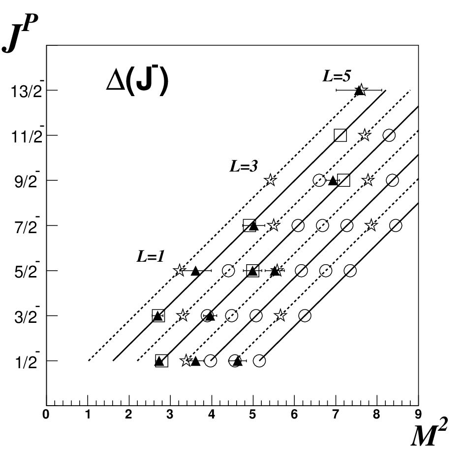
In Fig. 4 we demonstrate the setting of baryons on the $(J^{P},M^{2})$ planes. We see reasonably good description of data, although the scheme requires some additional states as well as double pole structures in many cases.

The deciphering of baryon setting shown in Fig. 4 is given in (50), (51), (52), (53) – the mass values (in MeV units) are taken from [22, 38, 39, 40].

Let us comment the trajectories in Fig. 4. The states belonging to the same $J^{P}$ trajectories have $\delta J^{\pm}=2^{\pm}$ and $M^{2}_{(J+2)^{\pm}}-M^{2}_{J^{\pm}}\simeq 2$ GeV². Clear examples give us $\Delta(\frac{3}{2}^{+})$ trajectory (the states $\Delta_{\frac{3}{2}^{+}}(1231)$ , $\Delta_{\frac{7}{2}^{+}}(1895)$ , $\Delta_{\frac{11}{2}^{+}}(2400)$ , $\Delta_{\frac{13}{2}^{+}}(2920)$ ) and $N(\frac{5}{2}^{-})$ trajectory (the states $N_{\frac{5}{2}^{-}}(1670)$ , $N_{\frac{9}{2}^{-}}(2250)$ , $N_{\frac{13}{2}^{-}}(2270)$ ). At the same time, in Fig. 4 we see the lines with $\delta J^{\pm}=1^{\pm}$ and $M^{2}_{(J+2)^{\pm}}-M^{2}_{J^{\pm}}\simeq 1$ GeV²: actually, such a line represents two overlapping trajectories.

For better presentation of the model, let us re-draw the ( $J,M^{2}$ ) planes keeping the basic ( $n=1$ ) states only – they are shown in Fig. 5.

For $L=0$ we see two basic states: $N(1/2^{+})$ and $\Delta(3/2^{+})$ .

In the $I=3/2$ sector we have five states for $L=1$ and six states for each $L$ at $L>1$ .

For ( $L=1,\,I=1/2$ ) states we have five basic states with $J^{P}=\frac{1}{2}^{-},\;\frac{3}{2}^{-},\quad J^{P}=\frac{1}{2}^{-},\;\frac{3}{2}^{-},\;\frac{5}{2}^{-},\quad J^{P}=\frac{1}{2}^{-},\;\frac{3}{2}^{-}$ , while for the states with $L>1$ we have $J^{P}=(L+\frac{1}{2})^{P},\;(L-\frac{1}{2})^{P},\quad J^{P}=(L+\frac{3}{2})^{P},\;(L+\frac{1}{2})^{P},\;(L-\frac{1}{2})^{P},\;(L-\frac{3}{2})^{P},\quad J^{P}=(L+\frac{1}{2})^{P},\;(L-\frac{1}{2})^{P}$ .

The states belonging to the same trajectory have $\delta J^{\pm}=2^{\pm}$ and $M^{2}_{(J+2)^{\pm}}-M^{2}_{J^{\pm}}\simeq 2$ GeV². One pair of states with $S=\frac{1}{2}$ and $I=\frac{1}{2}$ is formed by the $D_{0}^{0}$ diquark – we cannot assert definitely what pair is built by $D_{0}^{0}$ , heavier or lighter one.

4.1 The setting of $N(J^{+})$ states at $M_{D^{0}_{0}}\neq M_{D^{1}_{1}}$ and $L\geq 2$

In this sector the trajectories of Fig. 4 give us the following states at $L\geq 2$ :

$L=2$	$S=\frac{1}{2}$			$N(\frac{3}{2}^{+})$	$N(\frac{5}{2}^{+})$
		$n=1$		$(1720\pm 30)$	$(1685\pm 5)$
		$n=2$		$\sim 2040^{(*)}$	$(2000\pm 100)$
		$n=3$		$\sim 2300^{(*)}$	$\sim 2300^{(*)}$
		$n=4$		$\sim 2530^{(*)}$	$\sim 2530^{(*)}$
	$S=\frac{1}{2}$			$N(\frac{3}{2}^{+})$	$N(\frac{5}{2}^{+})$
		$n=1$		$\sim 2040^{(*)}$	$\sim 2040$
		$n=2$		$\sim 2300^{(*)}$	$\sim 2300^{(*)}$
		$n=3$		$\sim 2530^{(*)}$	$\sim 2530^{(*)}$
		$n=4$		$\sim 2740$	$\sim 2740^{(*)}$
	$S=\frac{3}{2}$		$N(\frac{1}{2}^{+})$	$N(\frac{3}{2}^{+})$	$N(\frac{5}{2}^{+})$	$N(\frac{7}{2}^{+})$
		$n=1$	$(1880\pm 40)$	$(1915\pm 50)$	$\sim 1900$	$(1990\pm 80)$
		$n=2$	$\sim 2180$	$\sim 2180$	$\sim 2170$	$\sim 2170$
		$n=3$	$\sim 2420$	$\sim 2420$	$\sim 2420^{(*)}$	$\sim 2410^{(*)}$
		$n=4$	$\sim 2640$	$\sim 2640$	$\sim 2640^{(*)}$	$\sim 2630^{(*)}$
$L=4$	$S=\frac{1}{2}$			$N(\frac{7}{2}^{+})$	$N(\frac{9}{2}^{+})$
		$n=1$		$\sim 2290$	$(2260\pm 60)$
		$n=2$		$\sim 2520$	$\sim 2520^{(*)}$
		$n=3$		$\sim 2740^{(*)}$	$\sim 2730^{(*)}$
		$n=4$		$\sim 2930^{(*)}$	$\sim 2930^{(*)}$
	$S=\frac{1}{2}$			$N(\frac{7}{2}^{+})$	$N(\frac{9}{2}^{+})$
		$n=1$		$\sim 2520$	$\sim 2520^{(*)}$
		$n=2$		$\sim 2740^{(*)}$	$\sim 2730^{(*)}$
		$n=3$		$\sim 2930^{(*)}$	$\sim 2930^{(*)}$
	$S=\frac{3}{2}$		$N(\frac{5}{2}^{+})$	$N(\frac{7}{2}^{+})$	$N(\frac{9}{2}^{+})$	$N(\frac{11}{2}^{+})$
		$n=1$	$\sim 2420^{(*)}$	$\sim 2410^{(*)}$	$\sim 2410$	$\sim 2400$
		$n=2$	$\sim 2640^{(*)}$	$\sim 2630^{(*)}$	$\sim 2630$	$\sim 2630$
		$n=3$	$\sim 2840^{(*)}$	$\sim 2840^{(*)}$	$\sim 2830^{(*)}$	$\sim 2830^{(*)}$
$L=6$	$S=\frac{1}{2}$			$N(\frac{11}{2}^{+})$	$N(\frac{13}{2}^{+})$
		$n=1$		$\sim 2730$	$(2700\pm 100)$
		$n=2$		$\sim 2930$	$\sim 2920$
	$S=\frac{1}{2}$			$N(\frac{11}{2}^{+})$	$N(\frac{13}{2}^{+})$
		$n=1$		$\sim 2930$	$\sim 2920$
		$n=2$		$\sim 3110$	$\sim 3110$
	$S=\frac{3}{2}$		$N(\frac{9}{2}^{+})$	$N(\frac{11}{2}^{+})$	$N(\frac{13}{2}^{+})$	$N(\frac{15}{2}^{+})$
		$n=1$	$\sim 2830^{(*)}$	$\sim 2830^{(*)}$	$\sim 2830$	$\sim 2820$
		$n=2$	$\sim 3020^{(*)}$	$\sim 3020^{(*)}$	$\sim 3020$	$\sim 3010$

(50)

The symbol ^(∗) means that in this mass region we should have two poles.

We see reasonable agreement of our predictions with data.

4.2 The setting of the $N(J^{-})$ states at $M_{D^{0}_{0}}\neq M_{D^{1}_{1}}$

In the $N(J^{-})$ sector the lightest states have $L=1$ , and we see that these states are in agreement with model predictions. But let us stress that the scheme requires a series of radial excitation states at $J^{P}=\frac{1}{2}^{+},\frac{3}{2}^{+},\frac{5}{2}^{+}$ at $M\simeq 2010$ MeV.

$L=1$	$S=\frac{1}{2}$			$N(\frac{1}{2}^{-})$	$N(\frac{3}{2}^{-})$
		$n=1$		$(1530\pm 30)$	$(1524\pm 5)$
		$n=2$		$(1905\pm 60)$	$(1875\pm 25)$
		$n=3$		$(2180\pm 80)^{(*)}$	$(2160\pm 40)^{(*)}$
		$n=4$		$\sim 2390^{(*)}$	$\sim 2390^{(*)}$
	$S=\frac{1}{2}$			$N(\frac{1}{2}^{-})$	$N(\frac{3}{2}^{-})$
		$n=1$		$\sim 1870$	$\sim 1860$
		$n=2$		$\sim 2140^{(*)}$	$\sim 2140^{(*)}$
		$n=3$		$\sim 2390^{(*)}$	$\sim 2390^{(*)}$
		$n=4$		$\sim 2610^{(*)}$	$\sim 2610^{(*)}$
	$S=\frac{3}{2}$			$N(\frac{1}{2}^{-})$	$N(\frac{3}{2}^{-})$	$N(\frac{5}{2}^{-})$
		$n=1$		$(1705\pm 30)$	$(1740\pm 20)$	$(1670\pm 20)$
		$n=2$		$\sim 2010$	$\sim 2000$	$\sim 2000$
		$n=3$		$\sim 2270$	$\sim 2270^{(*)}$	$\sim 2260^{(*)}$
		$n=4$		$\sim 2500$	$\sim 2500^{(*)}$	$\sim 2500^{(*)}$
$L=3$	$S=\frac{1}{2}$			$N(\frac{5}{2}^{-})$	$N(\frac{7}{2}^{-})$
		$n=1$		$(2150\pm 80)$	$(2170\pm 50)$
		$n=2$		$\sim 2380^{(*)}$	$\sim 2380^{(*)}$
		$n=3$		$\sim 2610^{(*)}$	$\sim 2600^{(*)}$
		$n=4$		$\sim 2810^{(*)}$	$\sim 2810^{(*)}$
	$S=\frac{1}{2}$			$N(\frac{5}{2}^{-})$	$N(\frac{7}{2}^{-})$
		$n=1$		$\sim 2380^{(*)}$	$\sim 2380^{(*)}$
		$n=2$		$\sim 2610^{(*)}$	$\sim 2600^{(*)}$
		$n=3$		$\sim 2810^{(*)}$	$\sim 2810^{(*)}$
	$S=\frac{3}{2}$		$N(\frac{3}{2}^{-})$	$N(\frac{5}{2}^{-})$	$N(\frac{7}{2}^{-})$	$N(\frac{9}{2}^{-})$
		$n=1$	$\sim 2270^{(*)}$	$\sim 2260^{(*)}$	$\sim 2260$	$(2250\pm 50)$
		$n=2$	$\sim 2500^{(*)}$	$\sim 2500^{(*)}$	$\sim 2490$	$\sim 2490$
		$n=3$	$\sim 2720^{(*)}$	$\sim 2710^{(*)}$	$\sim 2710^{(*)}$	$\sim 2700^{(*)}$
$L=5$	$S=\frac{1}{2}$			$N(\frac{9}{2}^{-})$	$N(\frac{11}{2}^{-})$
		$n=1$		$\sim 2600$	$\sim 2600$
		$n=2$		$\sim 2810^{(*)}$	$\sim 2800^{(*)}$
		$n=3$		$\sim 3000^{(*)}$	$\sim 3000^{(*)}$
	$S=\frac{1}{2}$			$N(\frac{9}{2}^{-})$	$N(\frac{11}{2}^{-})$
		$n=1$		$\sim 2810^{(*)}$	$\sim 2800^{(*)}$
		$n=2$		$\sim 3000^{(*)}$	$\sim 3000^{(*)}$
	$S=\frac{3}{2}$		$N(\frac{7}{2}^{-})$	$N(\frac{9}{2}^{-})$	$N(\frac{11}{2}^{-})$	$N(\frac{13}{2}^{-})$
		$n=1$	$\sim 2710^{(*)}$	$\sim 2700^{(*)}$	$\sim 2700$	$\sim 2700$
		$n=2$	$\sim 2910^{(*)}$	$\sim 2900^{(*)}$	$\sim 2900$	$\sim 2900$

(51)

4.3 The setting of $\Delta(J^{+})$ states at $M_{D^{0}_{0}}\neq M_{D^{1}_{1}}$ and $L\geq 2$

Considering the equation (52), we should remember that the ( $L=0$ ) states are excluded from the suggested classification – they are given in section 3.

$L=2$	$S=\frac{1}{2}$			$\Delta(\frac{3}{2}^{+})$	$\Delta(\frac{5}{2}^{+})$
		$n=1$		$\sim 1760$	$\sim 1760$
		$n=2$		$\sim 2060$	$\sim 2050$
		$n=3$		$\sim 2310$	$\sim 2310$
		$n=4$		$\sim 2540$	$\sim 2540$
	$S=\frac{3}{2}$		$\Delta(\frac{1}{2}^{+})$	$\Delta(\frac{3}{2}^{+})$	$\Delta(\frac{5}{2}^{+})$	$\Delta(\frac{7}{2}^{+})$
		$n=1$	$(1895\pm 25)$	$(1990\pm 35)^{(*)}$	$(1890\pm 25)$	$(1895\pm 20)$
		$n=2$	$\sim 2190$	$\sim 2190^{(*)}$	$\sim 2180$	$\sim 2180$
		$n=3$	$\sim 2430$	$\sim 2430^{(*)}$	$\sim 2430^{(*)}$	$\sim 2420^{(*)}$
		$n=4$	$\sim 2650$	$\sim 2650^{(*)}$	$\sim 2650^{(*)}$	$\sim 2640^{(*)}$
$L=4$	$S=\frac{1}{2}$			$\Delta(\frac{7}{2}^{+})$	$\Delta(\frac{9}{2}^{+})$
		$n=1$		$\sim 2300$	$\sim 2300$
		$n=2$		$\sim 2530$	$\sim 2530$
		$n=3$		$\sim 2750$	$\sim 2740$
		$n=4$		$\sim 2940$	$\sim 2940$
	$S=\frac{3}{2}$		$\Delta(\frac{5}{2}^{+})$	$\Delta(\frac{7}{2}^{+})$	$\Delta(\frac{9}{2}^{+})$	$\Delta(\frac{11}{2}^{+})$
		$n=1$	$\sim 2430^{(*)}$	$(2390\pm 100)^{(*)}$	$(2400\pm 50)$	$(2420\pm 100)$
		$n=2$	$\sim 2650^{(*)}$	$\sim 2640^{(*)}$	$\sim 2640$	$\sim 2640$
		$n=3$	$\sim 2850^{(*)}$	$\sim 2850^{(*)}$	$\sim 2840^{(*)}$	$\sim 2840^{(*)}$
		$n=4$	$\sim 3040^{(*)}$	$\sim 3040^{(*)}$	$\sim 3030^{(*)}$	$\sim 3030^{(*)}$
$L=6$	$S=\frac{1}{2}$			$\Delta(\frac{11}{2}^{+})$	$\Delta(\frac{13}{2}^{+})$
		$n=1$		$\sim 2740$	$\sim 2740$
		$n=2$		$\sim 2940$	$\sim 2930$
		$n=3$		$\sim 3120$	$\sim 3120$
		$n=4$		$\sim 3300$	$\sim 3290$
	$S=\frac{3}{2}$		$\Delta(\frac{9}{2}^{+})$	$\Delta(\frac{11}{2}^{+})$	$\Delta(\frac{13}{2}^{+})$	$\Delta(\frac{15}{2}^{+})$
		$n=1$	$\sim 2840^{(*)}$	$\sim 2840^{(*)}$	$\sim 2840$	$(2920\pm 100)$
		$n=2$	$\sim 3030^{(*)}$	$\sim 3030^{(*)}$	$\sim 3030$	$\sim 3020$
		$n=3$	$\sim 3210^{(*)}$	$\sim 3210^{(*)}$	$\sim 3210$	$\sim 3200$
		$n=4$	$\sim 3380^{(*)}$	$\sim 3380^{(*)}$	$\sim 3380$	$\sim 3370$

(52)

4.4 The setting of $\Delta(J^{-})$ states at $M_{D^{0}_{0}}\neq M_{D^{1}_{1}}$

In the $\Delta(J^{-})$ sector we face a problem with the $\frac{5}{2}^{-}$ state observed in the analysis [34] with mass 2233 MeV and quoted as $D_{35}(1930)$ [22]. However, it can be hardly compatible with other observations, which are in the region of 1930 MeV. In addition, the result of [34] is compatible with the analysis of Manley [24], quoted by PDG as $D_{35}(2350)$ . Thus, we introduce the $\Delta(\frac{5}{2}^{-})$ state with the mass 2210 MeV and with the error which covers the results of [24, 34]. Then, the mass of the $D_{35}(2350)$ state is taken as an average value over the results of [23, 25, 29].

$L=1$	$S=\frac{1}{2}$			$\Delta(\frac{1}{2}^{-})$	$\Delta(\frac{3}{2}^{-})$
		$n=1$		$(1650\pm 25)$	$(1640\pm 40)$
		$n=2$		$(1900\pm 50)$	$(1990\pm 40)$
		$n=3$		$(2150\pm 50)$	$\sim 2210$
		$n=4$		$\sim 2460$	$\sim 2450$
	$S=\frac{3}{2}$			$\Delta(\frac{1}{2}^{-})$	$\Delta(\frac{3}{2}^{-})$	$\Delta(\frac{5}{2}^{-})$
		$n=1$		$\sim 1800$	$\sim 1800$	$(1910\pm 80)$
		$n=2$		$\sim 2090$	$\sim 2080$	$\sim 2080$
		$n=3$		$\sim 2340$	$\sim 2340^{(*)}$	$\sim 2330^{(*)}$
		$n=4$		$\sim 2570$	$\sim 2560^{(*)}$	$\sim 2560^{(*)}$
$L=3$	$S=\frac{1}{2}$			$\Delta(\frac{5}{2}^{-})$	$\Delta(\frac{7}{2}^{-})$
		$n=1$		$\sim 2210$	$(2240\pm 60)$
		$n=2$		$\sim 2450$	$\sim 2440$
		$n=3$		$\sim 2670$	$\sim 2660$
	$S=\frac{3}{2}$		$\Delta(\frac{3}{2}^{-})$	$\Delta(\frac{5}{2}^{-})$	$\Delta(\frac{7}{2}^{-})$	$\Delta(\frac{9}{2}^{-})$
		$n=1$	$\sim 2340^{(*)}$	$(2350\pm 50)^{(*)}$	$\sim 2330$	$\sim 2320$
		$n=2$	$\sim 2560^{(*)}$	$\sim 2560^{(*)}$	$\sim 2560$	$\sim 2550$
		$n=3$	$\sim 2770^{(*)}$	$\sim 2770^{(*)}$	$\sim 2770^{(*)}$	$\sim 2760^{(*)}$
$L=5$	$S=\frac{1}{2}$			$\Delta(\frac{9}{2}^{-})$	$\Delta(\frac{11}{2}^{-})$
		$n=1$		$(2633\pm 30)$	$\sim 2660$
		$n=2$		$\sim 2860$	$\sim 2860$
		$n=3$		$\sim 3050$	$\sim 3050$
	$S=\frac{3}{2}$		$\Delta(\frac{7}{2}^{-})$	$\Delta(\frac{9}{2}^{-})$	$\Delta(\frac{11}{2}^{-})$	$\Delta(\frac{13}{2}^{-})$
		$n=1$	$\sim 2770^{(*)}$	$\sim 2760^{(*)}$	$\sim 2760$	$(2750\pm 100)$
		$n=2$	$\sim 2960^{(*)}$	$\sim 2960^{(*)}$	$\sim 2950$	$\sim 2950$
		$n=3$	$\sim 3140^{(*)}$	$\sim 3140^{(*)}$	$\sim 3140$	$\sim 3140$

(53)

4.5 Overlapping of baryon resonances

In equations (50), (51), (52), (53), the overlapping resonances are denoted by the symbol $(^{*})$ – the model predicts a lot of such states. Decay processes lead to a mixing of the overlapping states (owing to the transition $baryon(1)\to hadrons\to baryon(2)$ ). It results in a specific phenomenon, that is, when several resonances overlap, one of them accumulates the widths of neighbouring resonances and transforms into the broad state, see [17, 41] and references therein.

This phenomenon had been observed in [42, 43] for meson scalar–isoscalar states and applied to the interpretation of the broad state $f_{0}(1200-1600)$ , being a descendant of a pure glueball [44, 45].

In meson physics this phenomenon can play an important role, in particular, for exotic states which are beyond the $q\bar{q}$ systematics. Indeed, being among $q\bar{q}$ resonances, the exotic state creates a group of overlapping resonances. The exotic state, after accumulating the ”excess” of widths, turns into a broad one. This broad resonance should be accompanied by narrow states which are the descendants of states from which the widths have been borrowed. In this way, the existence of a broad resonance accompanied by narrow ones may be a signature of exotics. This possibility, in context of searching for exotic states, was discussed in [46].

In the considered case of quark–diquarks baryons (equations (50), (51), (52), (53)), we deal mainly with two overlapping states: it means that we should observe one comparatively narrow resonance together with the second one which is comparatively broad. Experimental observation of the corresponding two-pole singularities in partial amplitudes looks as rather intricate problem.

4.5.1 The setting of baryons with $M_{D^{0}_{0}}\neq M_{D^{1}_{1}}$ on $(n,M^{2})$ planes

Equations (50), (51), (52), (53) allow us to present the setting of baryons ( $M_{D^{0}_{0}}\neq M_{D^{1}_{1}}$ ) on $(n,M^{2})$ planes – they are shown in Figs. 6 and 7.

We have three trajectories on the $(n,M^{2})$ plot for $N(\frac{1}{2}^{+})$ with the starting states shown in Fig. 5 in the $L=0$ group. The low trajectory is filled in by the states of equation (49).

In the plot for $N(\frac{3}{2}^{+})$ we also have three trajectories, with the starting $L=2$ states, see Fig. 5. Likewise, all other $(n,M^{2})$ plots are constructed: the starting states are those shown in Fig. 5.

We have a lot of predicted radial excitation states, though not many observed ones – the matter is that in case of overlapping resonances the broad state is concealed under narrow one. As is well known, the mixing states repulse from one another. The mixing of overlapping states, due to the transition into real hadrons $baryon(1)\to real\;hadrons\to baryon(2)$ also leads to the repulsing of resonance poles in the complex- $M$ plane: one is moving to real $M$ axis (i.e. reducing the width), another is diving deaper into complex- $M$ plane (i.e. increasing the width) – for more detail see [17], sections 3.4.2 and 3.4.3. To separate two overlapping poles, one needs to carry out the measurements of decays into different channels – different resonances have, as a rule, different partial widths, so the total width of the ”two-pole resonance” should depend on the reaction type.

Radially excited states are seen in (see Figs. 6 and 7), namely,
$N(\frac{1}{2}^{+})$ sector (four states on the lowest trajectory),
$N(\frac{5}{2}^{+})$ sector (two states on the lowest trajectory),
$N(\frac{1}{2}^{-})$ sector (three states on the lowest trajectory),
$N(\frac{3}{2}^{-})$ sector (three states on the lowest trajectory),
$\Delta(\frac{3}{2}^{+})$ sector (three states on the lowest trajectory),
$\Delta(\frac{1}{2}^{-})$ sector (three states on the lowest trajectory),
$\Delta(\frac{3}{2}^{-})$ sector (two states on the lowest trajectory),
$\Delta(\frac{5}{2}^{-})$ sector (two states on the lowest trajectory).

However, in Figs. 6 and 7 we do not mark specially the resonances which are ”shadowed” by observed ones. The slopes of all trajectories in Figs. 6 and 7 coincide with each other and with those of meson trajectories (see [17, 37]).

5 A variant with $M_{D^{0}_{0}}=M_{D^{1}_{1}}$ and overlapping $qD^{0}_{0}(S=1/2)$ and $qD^{1}_{1}(S=1/2)$ states

Here we consider the case with further decrease of states which can be easily seen. We suppose that $M_{D^{0}_{0}}=M_{D^{1}_{1}}$ and the states $qD^{0}_{0}(S=1/2)$ and $qD^{1}_{1}(S=1/2)$ overlap. So, for a naive observer, who does not perform an analysis of double pole structure, the number of states with $S=1/2$ decreases twice.

In Fig. 8 we show $(J,M^{2})$ plots as they look like for ”naive observers”, while Fig. 9 demonstrates the $(J,M^{2})$ plots for ground states ( $n=1$ ) only.

Figures 8, 9 present us more compact scheme than that given in Figs. 4, 5.

6 Conclusion

We have systematized all baryon states in the framework of the hypothesis of their quark–diquark structure. We cannot say whether such a systematization is unambiguous, so we discuss possible versions of setting baryons upon multiplets. To carry out a more definite systematization, additional efforts are needed in both experiment and phenomenological comprehension of data.

Concerning the experiment, it is necessary:
(i) To investigate in details the $\Delta$ spectrum in the region around 1700 MeV. Here one should search for the $D_{15}$ and/or $F_{15}$ states. The double pole structures should be searched for, first, in the regions $N_{\frac{1}{2}^{+}}(1400)$ and $\Delta_{\frac{3}{2}^{+}}(1600)$ .
(ii) To increase the interval of available energies in order to get a possibility to investigate resonances up to the masses 3.0–3.5 GeV.
(iii) To measure various types of reactions in order to analyze them simultaneously.

As to the phenomenology and theory, it is necessary to continue the $K$ -matrix analysis, the first results of which were obtained in [35, 47], in order to cover a larger mass interval and the most possible number of reactions. One should take into account the expected overlapping of resonances. Namely, the standard procedure should be elaborated for singling out the amplitude poles in the complex- $M$ plane in case when one pole is under another.

We thank L.G. Dakhno and E. Klempt for helpful discussions. This paper was supported by the grants RFBR No 07-02-01196-a and RSGSS-3628.2008.2.

References

[1] V.V. Anisovich, Pis’ma ZhETF 2, 439 (1965) [JETP Lett. 2, 272 (1965)].
[2] M. Ida and R. Kobayashi, Progr. Theor. Phys. 36, 846 (1966).
[3] D.B Lichtenberg and L.J. Tassie, Phys. Rev. 155, 1601 (1967).
[4] S. Ono, Progr. Theor. Phys. 48 964 (1972).
[5] V.V. Anisovich, Pis’ma ZhETF 21 382 (1975) [JETP Lett. 21, 174 (1975)];
V.V. Anisovich, P.E. Volkovitski, and V.I. Povzun, ZhETF 70, 1613 (1976) [Sov. Phys. JETP 43, 841 (1976)].
[6] A. Schmidt and R. Blankenbeckler, Phys. Rev. D16, 1318 (1977).
[7] F.E Close and R.G. Roberts, Z. Phys. C 8, 57 (1981).
[8] T. Kawabe, Phys. Lett. B 114, 263 (1982).
[9] S. Fredriksson, M. Jandel, and T. Larsen, Z. Phys. C 14, 35 (1982).
[10] M. Anselmino and E. Predazzi, eds., Proceedings of the Workshop on Diquarks, World Scientific, Singapore (1989).
[11] K. Goeke, P.Kroll, and H.R. Petry, eds., Proceedings of the Workshop on Quark Cluster Dynamics (1992).
[12] M. Anselmino and E. Predazzi, eds., Proceedings of the Workshop on Diquarks II, World Scientific, Singapore (1992).
[13] N. Izgur and G. Karl, Phys. Rev. D18, 4187 (1978); D19, 2653 (1979);
S. Capstik, N. Izgur, Phys. Rev. D34, 2809 (1986).
[14] L.Y. Glozman et al., Phys. Rev. D58:094030 (1998).
[15] U. Löring, B.C. Metsch, H.R. Petry, Eur.Phys. A10, 395 (2001); A10, 447 (2001).
[16] V.V. Anisovich, M.N. Kobrinsky, J. Nyiri, Yu.M. Shabelski Quark Model and High Energy Collisions , Second Edition, World Scientific, Singapore, 2004.
[17] A.V. Anisovich, V.V. Anisovich, J. Nyiri, V.A. Nikonov, M.A. Matveev and A.V. Sarantsev, Mesons and Baryons. Systematization and Methods of Analysis, World Scientific, Singapore, 2008.
[18] V.V. Anisovich, D.I. Melikhov, V.A. Nikonov, Yad. Fiz. 57, 520 (1994) [Phys. Atom. Nucl. 57, 490 (1994)]
[19] V.V. Anisovich, E.M. Levin and M.G. Ryskin, Yad. Fiz. 29, 1311 (1979); [Phys. Atom. Nuclei 29, 674 (1979)].
[20] G. Källen, Helv. Phys. Acta. 25, 417 (1952);
H. Lehman, Nuovo Cim. 11, 342 (1952).
[21] V.V. Anisovich, S.M. Gerasyuta, A.V. Sarantsev, Int. J. Mod. Phys. A6, 625 (1991).
[22] C. Amsler et al. [Particle Data Group], Phys. Lett. B 667 (2008) 1.
[23] R. E. Cutkosky, C. P. Forsyth, J. B. Babcock, R. L. Kelly and R. E. Hendrick,
[24] D. M. Manley and E. M. Saleski, Phys. Rev. D 45, 4002 (1992).
[25] T. P. Vrana, S. A. Dytman and T. S. H. Lee, Phys. Rept. 328, 181 (2000) [arXiv:nucl-th/9910012].
[26] R. Plotzke et al. [SAPHIR Collaboration], Phys. Lett. B 444 (1998) 555.
[27] K. W. Bell et al., Nucl. Phys. B 222, 389 (1983).
[28] A. V. Sarantsev, V. A. Nikonov, A. V. Anisovich, E. Klempt and U. Thoma, Eur. Phys. J. A 25, 441 (2005) [arXiv:hep-ex/0506011].
[29] G. Hohler, In Bratislava 1973, Proceedings, Triangle Meeting On Hadron Interactions At Low Energies, Bratislava 1975, 11-75.
[30] A. V. Anisovich, V. Kleber, E. Klempt, V. A. Nikonov, A. V. Sarantsev and U. Thoma, Eur. Phys. J. A 34, 243 (2007) [arXiv:0707.3596 [hep-ph]].
[31] M. Ablikim et al., Phys. Rev. Lett. 97, 262001 (2006) [arXiv:hep-ex/0612054].
[32] M. Batinic, I. Slaus, A. Svarc and B. M. K. Nefkens, Phys. Rev. C 51, 2310 (1995) [Erratum-ibid. C 57, 1004 (1998)] [arXiv:nucl-th/9501011].
[33] V. Crede et al. [CB-ELSA Collaboration], Phys. Rev. Lett. 94, 012004 (2005) [arXiv:hep-ex/0311045].
[34] R. A. Arndt, W. J. Briscoe, I. I. Strakovsky and R. L. Workman, Phys. Rev. C 74, 045205 (2006) [arXiv:nucl-th/0605082].
[35] I. Horn et al. [CB-ELSA Collaboration], Phys. Rev. Lett. 101, 202002 (2008) [arXiv:0711.1138 [nucl-ex]].
[36] I. Horn et al. [CB-ELSA Collaboration], Eur. Phys. J. A 38, 173 (2008) [arXiv:0806.4251 [nucl-ex]].
[37] A.V. Anisovich, V.V. Anisovich, and A.V. Sarantsev, Phys. Rev. D 62:051502(R) (2000).
[38] A.V. Anisovich, E. Klempt, V.A. Nikonov et al. arXiv: hep-ph:0911.5277.
[39] A.V. Sarantsev et al. Phys. Lett. B 659:94-100 (2008)
[40] A.V. Anisovich, I.Jaegle, E. Klempt et al. Eur. Phys. J. A 41:13-44 (2009)
[41] V.V. Anisovich, UFN, 174, 49 (2004) [Physics-Uspekhi, 47, 45 (2004)].
[42] V.V.Anisovich and A.V.Sarantsev, Int. J. Mod. Phys. A24, 2481 (2009).
[43] V.V.Anisovich and A.V.Sarantsev, Phys. Lett. B 382, 429 (1996).
[44] A.V.Anisovich, V.V.Anisovich, Yu.D.Prokoshkin, and A.V.Sarantsev, Zeit. Phys. A 357, 123 (1997).
[45] A.V.Anisovich, V.V.Anisovich, and A.V.Sarantsev, Phys. Lett. B 395, 123 (1997); Zeit. Phys. A 359, 173 (1997).
[46] V.V.Anisovich, D.V.Bugg, and A.V.Sarantsev, Phys. Rev. D 58:111503 (1998).
[47] U. Thoma et al., Phys. Lett. B 659 (2008) 87 [arXiv:0707.3592 [hep-ph]].

Searching for the quark–diquark systematics of baryons composed by light quarks q=u,dq=u,d

Abstract

1 Introduction

2 Baryons as quark–diquark systems

2.1 SS-wave diquarks and baryons

2.2 Wave functions of quark–diquark systems with L=0L=0

2.2.1 The Δ\Delta isobar: quark–diquark wave function for arbitrary nn and its transformation into the S​U​(6)SU(6) wave function

2.2.2 The state with I=3/2I=3/2, J=1/2J=1/2 at L=0L=0 and S=1/2S=1/2, ΔJP=12+​(L=0,S=1/2)\Delta_{J^{P}=\frac{1}{2}^{+}}(L=0,S=1/2)

2.2.3 The nucleon N1/2N_{1/2}: quark–diquark wave function for arbitrary nn and its transformation into the S​U​(6)SU(6) one

2.2.4 The state with I=1/2I=1/2, J=3/2J=3/2, L=0L=0 and S=3/2S=3/2, NJP=32+​(L=0,S=3/2)N_{J^{P}=\frac{3}{2}^{+}}(L=0,S=3/2)

2.3 Wave functions of quark–diquark systems with L≠0L\neq 0