Joint Scheduling and ARQ for MU-MIMO Downlink in the Presence of Inter-Cell Interference
Abstract
User scheduling and multiuser multi-antenna (MU-MIMO) transmission are at the core of high-rate data-oriented downlink schemes of the next-generation of cellular systems (e.g., LTE-Advanced). Scheduling selects groups of users according to their channels vector directions and SINR levels. However, when scheduling is applied independently in each cell, the inter-cell interference (ICI) power at each user receiver is not known in advance since it changes at each new scheduling slot depending on the scheduling decisions of all interfering base stations. In order to cope with this uncertainty, we consider the joint operation of scheduling, MU-MIMO beamforming and Automatic Repeat reQuest (ARQ). We develop a game-theoretic framework for this problem and build on stochastic optimization techniques in order to find optimal scheduling and ARQ schemes. Particularizing our framework to the case of “outage service rates”, we obtain a scheme based on adaptive variable-rate coding at the physical layer, combined with ARQ at the Logical Link Control (ARQ-LLC). Then, we present a novel scheme based on incremental redundancy Hybrid ARQ (HARQ) that is able to achieve a throughput performance arbitrarily close to the “genie-aided service rates”, with no need for a genie that provides non-causally the ICI power levels. The novel HARQ scheme is both easier to implement and superior in performance with respect to the conventional combination of adaptive variable-rate coding and ARQ-LLC.
Keywords: Multiuser MIMO, inter-cell interference, scheduling, hybrid ARQ, stochastic optimization, game theory.
I Introduction
High-rate data-oriented downlink schemes [1, 2] have been successfully deployed as an extension of 3G cellular standards (WCDMA and CDMA2000). These schemes are based on the results of [3, 4, 5], showing that the throughput (or “ergodic”) sum-capacity of single-antenna multi-access (uplink) and broadcast (downlink) fading Gaussian channels is achieved by allocating opportunistically each time-frequency slot to the user with the best instantaneous channel conditions. In a multiuser setting, the sum-capacity is usually not the most meaningful measure of the system performance. Instead, maximizing the sum-throughput subject to some fairness constraint is more desirable [5]. To this purpose, a downlink scheduling policy can be designed in order to maximize a suitable concave and component-wise monotonically increasing network utility function over the system’s achievable throughput region (i.e., the region of achievable long-term average user rates). The network utility function is designed in order to capture the desired notion of “fairness” (e.g., proportional fairness, max-min fairness and, more in general, -fairness [6]).
In the next generation of cellular systems (e.g., the so-called LTE-Advanced [7]), high-rate data-oriented downlink schemes will be combined with multiuser multi-antenna (MU-MIMO) transmission techniques [8, 9], supporting spectral efficiencies in the 10’s of bits/sec/Hz [10, 11]. With MU-MIMO, the rate supported by each user is generally a function of all the user channel vectors, and depends on the type of MU-MIMO precoding [8, 9, 12]. In order to compute the transmitter precoder parameters (e.g., the beamforming steering vectors and the transmitted rates and powers), channel state information at the transmitter (CSIT) is required. This can be accurately obtained using open and closed loop channel estimation and feedback schemes (the literature on this subject is overwhelming, for example, see [13, 14, 15, 16, 17] and references therein).
In particular, scheduling with MU-MIMO and non-perfect CSIT was considered in [18], particularizing the general stochastic optimization framework of [19] to the case of a single-cell system with linear Zero-Forcing Beamforming (ZFBF) MU-MIMO precoding, where CSIT is obtained via noisy channel estimation and prediction.
In this work we focus on a multi-cell environment with no inter-cell cooperation. For sufficiently slowly-moving user terminals it is possible to design training and feedback schemes that achieve almost perfect CSIT [16, 17, 18]. Therefore, for simplicity we shall assume that each BS has perfect CSIT for its own users. In contrast, in a multi-cell system, inter-cell interference (ICI) emerges as another source of unavoidable uncertainty. (see [20, 21] and references therein). When the schedulers at each BS make their own decisions independently, based only on the locally available CSIT relative to their own users, the ICI power seen at each user receiver changes on a slot-by slot basis in a random and unpredictable manner, depending on the scheduling decision made at all the interfering BSs. As a consequence, the instantaneous Signal to Interference plus Noise Ratio (SINR) “seen” at any given user receiver is a random variable.
The decentralized scheduling problem in a multi-cell environment can be formulated as a non-cooperative game: each BS (player) wishes to maximize its own utility function over its own feasible throughput region. The players’ strategies are all feasible scheduling policies. In addition, the throughput region of any given cell depends on the ICI power statistics seen at the users’ receivers, which in turn depend on the scheduling policies applied at the interfering BSs. We show that when the individual network utility functions are concave the multi-cell decentralized scheduling game is a concave game and therefore Nash equilibria exist.
In order to solve the network utility maximization at each BS, for given ICI statistics, we apply the stochastic optimization framework of [19, 22, 23, 18]. A straightforward application of this approach yields a scheme based on variable-rate adaptive coding at the physical layer, and conventional ARQ at the Logical Link Control (LLC) layer. We notice that similar approaches are included in several wireless standards such as EV-DO and HSDPA [24, 25, 26], and therefore this can be regarded as the base-line “conventional” approach. In order to improve upon the conventional approach, we propose a new method based on combining incremental redundancy Hybrid Automatic Retransmission reQuest (HARQ) [27] and MU-MIMO opportunistic scheduling. In the proposed scheme, each user feeds back the value of the instantaneous mutual information observed in the previous slot, that is used by the scheduler to update recursively the scheduler weights. We show that the throughput achieved by the proposed HARQ scheme approaches the throughput of a “virtual system”, as if a genie provided non-causally the ICI values at each scheduling slot. However, we stress that the proposed scheme makes use of strictly causal information, and therefore requires no genie.
II System setup
We consider the downlink of a system with cells. In each cell, a BS equipped with with antennas transmits to single-antenna users. The channel is assumed frequency flat11 1 The generalization to MIMO-OFDM and frequency selective fading is immediate. and constant over “slots” of length symbols (block-fading model [28]). Any given channel use of the complex baseband discrete-time signal at the -th user in cell during slot is described by
| (1) |
where ticks at the slot rate, denotes user in cell , is the channel vector from the -th BS antenna array to the -th receiver antenna, is the signal transmitted by -th BS and is the additive white Gaussian noise (AWGN) sample. The coefficients are distance-dependent path gains [29] that are assumed to be time-invariant over many slots. The BSs are sum-power constrained such that for all , where denotes the transmit covariance matrix. The actual channel SNR is included as a common scaling factor in the coefficients . The channel vectors of users in cell form the columns of the channel matrix . We assume that all vectors are mutually independent with i.i.d. components , for all distinct 4-tuples . Each BS knows all time-invariant quantities relative to its own users and has perfect knowledge of immediately before the beginning of slot (perfect CSIT for the own users).
A feasible scheduling policy for BS is a possibly randomized stationary function22 2 Using the theory developed in [30] we can show that restricting to stationary policies does involve any suboptimality in terms of the achievable throughput region. that maps into the pair , where is a rate allocation vector. We assume that the MU-MIMO precoder is based on linear ZFBF. This yields the transmitted signal vector in the form , where denotes the set of active users, i.e., users that are selected to be served on slot and where denotes the coded symbol for user , with power . The ZFBF steering vectors are given by the unit-norm (normalized) -th column of the Moore-Penrose pseudoinverse (e.g., see [14, 31, 32, 16, 18] and references therein) of the channel matrix restricted to the active users, i.e., to the columns . It follows that the transmit covariance matrix takes on the form
| (2) |
where non-negative coefficients define the power allocation over the active users in cell , and satisfy the power constraint . A necessary and sufficient condition for perfect zero-forcing of the intra-cell multiuser interference is that . Without loss of generality, in the following we identify the set of active users with those users with positive powers, i.e., for and for .
The ICI power at user receiver in slot is given by
| (3) |
with mean given by . The SINR at user is given by
| (4) |
We let denote the instantaneous service rate of user on slot , measured in bits/channel use. This is in general a function of , and therefore of , and of the allocated rate . We define the -th user service rate function , such that . Let denote the set of all feasible scheduling policies and let denote the set of scheduling policies at all cells . For fixed , the throughput of user under the scheduling policy is given by
| (5) | |||||
where the effect of the policies at the interfering BSs is captured by the statistics of the ICI power process , the limit holds almost surely because of stationarity and ergodicity, and expectation is with respect to the joint distribution of the triple . 33 3 With some abuse of notation, we denote by and random variables whose joint distribution coincides with the first-order joint distribution of the processes and , which is time-invariant by stationarity. The region of achievable throughputs for cell is given by
| (6) |
“coh” denotes “closure of the convex hull”. Notice that depends on the other cells’ scheduling policies through the joint probability distribution of the ICI powers .
Under our assumptions, the BSs operate in a decentralized way and influence each other only in terms of the generated ICI statistics (i.e., the joint cdfs ). Each BS wishes to maximize its own network utility function. This multi-objective optimization problem is formulated as a non-cooperative game [33, 34] that we nickname the multi-cell decentralized scheduling game, where each player (i.e., BS) seeks to achieve
| maximize | |||||
| subject to | (7) |
where we assume that is a continuous, strictly concave and component-wise increasing utility function, reflecting some suitable fairness criterion [6].
By definition, for any given joint statistics of and of , the maximum in (7) is achieved by some scheduling policy . A Nash equilibrium of the decentralized scheduling game is a set of scheduling policies (also denoted, with some abuse of notation, by ) such that is the solution to (7) when , for all . We have:
Theorem 1
The decentralized scheduling game defined above is a concave game and therefore has a Nash equilibrium.
Proof:
All players have the same strategy set . This is a compact convex set due to the covariance trace constraint and to the fact that we can assume that the rate allocation vector is bounded in for some constant . 44 4 This limitation does not involve any significant loss of generality if is sufficiently large, and always holds in practice since practical variable-rate coding has a finite maximum rate. Also, each -th utility is a concave function of for fixed . In order to see this, let denote the throughput point of achieved by policy for fixed , consider any two policies and define as the policy that applies with probability and with probability . Then, from the convexity of and the concavity of we have that
Now, let and denote two vectors of scheduling policies and define the sum-utility function . Since the functions are continuous (by assumption) and the throughput vectors are continuous functions of the scheduling policies, it follows that is a continuous function of and, for what said before, it is concave in for any fixed . These properties match exactly the assumption of Rosen Theorem [35]. Therefore, as a direct consequence of [35], the existence of a Nash equilibrium is proved. ∎
Since is component-wise increasing, it follows that the maximum of (7) is obtained for some such that is on the Pareto boundary of . If the service rate function is strictly increasing in the power allocated to user , then the Pareto boundary of is achieved by policies that satisfy with probability 1. In this case, any Nash equilibrium must correspond to scheduling policies that achieve the power constraint with equality for all BSs.
In Sections III and IV we will focus on reference cell , assuming that all other interfering cells apply a fixed arbitrary policy (i.e., for fixed and known joint statistics of the ICI powers at all users of cell ). We shall apply the theory developed in [19, 18] and provide a stochastic optimization algorithm that solves (7) to any desired level of approximation, for any given ICI powers statistics.
III Scheduling with adaptive variable-rate coding and ARQ-LLC
From now on we shall assume Gaussian random coding and consider specific cases of service rate functions. In this case, we define the -th user mutual information function as
| (8) |
The mutual information at user receiver on slot is given by . We approximate the decoding error probability by the corresponding information outage probability (see [36, 28] for the information-theoretic motivations underlying this very common and very useful approximation). Namely, if the mutual information is less than the scheduled coding rate , the decoder makes a decoding error with probability close to 1, while if the random coding average error probability is very close to 0. Therefore, for slot length large enough, there exist “good” codes drawn from a Gaussian ensemble such that their block error probability is close to the information outage probability . In this case, the user service rate function is given by “outage rate” function [18]
| (9) |
In order to obtain the desired near-optimal scheduling policy, we apply the framework of [18]. We define the virtual queues55 5 It is important to keep in mind that the virtual queues have nothing to do with the ARQ transmission buffers: they are used here as a tool to recursively update the weights of the the scheduling policy. with buffer state and virtual arrival processes . The virtual queues evolve according to the stochastic difference equations
| (10) |
Then, we consider the adaptive policy defined by:
- 1.
For any given , let the transmit covariance matrix and the rate allocation vector be the solution of
(11) - 2.
For suitable constants , let the virtual arrival processes at time be given by the solution of
(12) - 3.
As stated in Theorem 2 below, the policy defined above achieves the optimal point solution of (7) within any desired accuracy, depending on the constants and . Neglecting the (small) degradation due to stochastic adaptation and quantified by Theorem 2, we shall refer to this policy as .
Theorem 2
Assume i.i.d. channels and fixed joint statistics of the ICI powers . Assume that is concave and entry-wise non-decreasing, and that there exists at least one point with strictly positive entries such that . Then, the scheduling policy defined above, for given constants and , has the following properties:
(a) The utility achieved by satisfies:
| (13) |
where
| (14) |
and where denotes the solution of the problem (7) with the additional constraint for all .
(b) For any point such that for all , and for any value we have:
| (15) |
Thus, all virtual queues are strongly stable.66 6 A discrete-time queue is strongly stable if . The system is strongly stable if all queues are strongly stable.
Proof:
The proof follows verbatim from the results in [18] and it is not repeated here for brevity. ∎
As a corollary of Theorem 2, if is sufficiently large such that for all , then satisfies
| (16) |
Hence, the control parameter can be chosen sufficiently large in order to make the achieved utility as close as desired to the optimal value of problem (7). This comes with a tradeoff in the virtual queue average sizes that, as seen from (15), grow linearly with . The virtual queue sizes represent the difference between the virtual bits admitted into the queues and the actual bits transmitted, and thus affect the time-scales required for the time averages to become close to their limiting values.
III-A Implementation
The policy found before computes recursively the “weights” via (12) and (10) and, for each , solves the weighted conditional average rate sum maximization (11). Problem (12) is a standard convex optimization problem the solution of which does not present any major conceptual difficulty and is found in closed form for the important cases of proportional fairness and max-min fairness (see [18]), corresponding to the choices and , respectively. In contrast, solving (11) presents some difficulties. Letting denote the marginal cdf of and using (8), the objective function in (11) can be rewritten as
| (17) |
The optimization in (11) is generally a non-convex problem that involves a combinatorial search over all subsets of cardinality and, for each candidate subset, the maximization of (17) with respect to and the power allocation . Since this optimization may be difficult to compute, we propose the following suboptimal low-complexity two-step approach:
Step 1) the active user subset and the corresponding power allocation are selected by assuming deterministic ICI powers, equal to their mean value . Under this assumption, the problem is reduced to the well-known user selection with ZFBF, that can be solved using standard techniques based on quasi-orthogonal user selection and waterfilling (e.g., [37, 38, 39]).
Step 2) for the transmit covariance obtained in step 1, (17) is optimized with respect to the rate allocation. This reduces to optimizing the outage rate separately for each by letting
| (18) |
where is fixed by Step 1.
Notice that, both in the original problem and in the proposed low-complexity two-step approximated solution, only the marginal statistics of the ICI powers are relevant. These marginal statistics can be measured by each user terminal individually and fed back to the BS scheduler by some very low-rate feedback scheme.
IV Scheduling with incremental redundancy HARQ
If a genie provides the BS scheduler with the values of the the mutual information in a non-causal fashion, just before the beginning of slot , then the optimal rate allocation would be, trivially, for all , yielding zero outage probability. This “genie-aided” case was considered in [18] and referred to as “optimistic rate” allocation, although no actual algorithm to approach the optimistic throughput was given. Since for any non-negative random variable and we have , then the optimistic service rates provide an upper bound to the throughput of any system with the same signaling scheme (ZFBF and Gaussian codes) and given rate allocation.
In this section we show how to achieve the “optimistic” throughput without the aid of any genie. As a preliminary step, let’s consider the following incremental redundancy HARQ scheme. The BS scheduler maintains a buffer of information packets for each user in the cell. The size of user packets is equal to bits per packet. Each packet is encoded into an infinite-length sequence of complex symbols.77 7 In practice, this rateless coding can be implemented by using Raptor codes [40]. The encoded sequence is partitioned into blocks of length symbols. At each slot , the scheduling policy computes according to some rule to be found later. For all active users , if the most recent HARQ feedback message from user is “NACK” (negative acknowledgement), then the first not-yet transmitted coded block of the current packet is transmitted. Otherwise, if the most recent received HARQ feedback message is “ACK” (positive acknowledgement), then the current packet is removed from the transmission buffer of user and the first coded block of next packet in the buffer is transmitted. The -th receiver stores in memory all the received slots for times and attempts to decode the current packet at every newly received slot, by using all the available received slots. If decoding fails, NACK is sent back, otherwise ACK is sent back and the decoder memory is reset. Notice that the scheme does not require any genie-aided “look-ahead” of the instantaneous ICI power , and makes use of time-invariant packet sizes . These may differ from user to user but are independent of . For later use, we define the “first-block coding rate” as the ratio bits/channel use.
Next, we describe a scheduling rule, denoted again by , that operates arbitrarily closely to the genie-aided throughput when combined with the HARQ scheme described above. At the end of each slot , the active users feed back both their ACK/NACK message and the mutual information “seen” at their receiver. Then, coincides with what given in Section III, after the following two changes. 1) The virtual queues evolution equation (10) is replaced by
| (19) |
2) The transmitter optimization (11) is replaced by
| (20) |
In brief, the scheduler updates recursively its weights and computes the transmitted signal covariance according to (20), as if it was operating on a virtual “genie-aided” system with instantaneous service rates . The throughput region of the virtual genie-aided system, denoted by , is given by (6), after replacing the general rate function with the mutual information function defined in (8). The performance of for the genie-aided system is again given by Theorem 2, where in (13) is replaced by the vector of mutual informations and where denotes the solution of (7) when is replaced by , with the additional constraint for all .
For sufficiently large , yields:
| (21) |
where is the utility-maximizing throughput point in the region . At this point, it remains to be shown that the combination of the policy with the incremental redundancy HARQ scheme yields a network utility as close as desired to the limit in (21). This is shown by the following:
Theorem 3
Let denote the throughput achievable by the incremental redundancy HARQ protocol under scheduling policy defined above. For each user and there exists a sufficiently large first-block rate such that .
Proof:
Consider user . Following the argument in [27], we can model the event of successful decoding as a “mutual information level-crossing event”. Suppose that the transmission of the current packet for user starts at slot (i.e., an ACK was fed back at slot time ). Then, the current packet can be successfully decoded at slot if . Otherwise, a decoding error occurs with very high probability. As shown in [27, 41], the probability of undetected decoding error vanishes exponentially with . Therefore, in the regime of large , if the decoding error is detected with arbitrarily high probability and a NACK is sent back. Fig. 1 shows, qualitatively, the mutual information level-crossing and the corresponding successful decoding events of the decoder. Notice that the mutual information increment is non-negative, and it is exactly zero for all such that , i.e., when user is not scheduled.
Consider the transmission of a long sequence of packets. Without loss of generality, assume that the system starts at time , denote by the number of successful decoding events of decoder up to time and let denote the corresponding “inter-ACK” times (see Fig. 1). Since at each successful decoding a “reward” of bit per channel use is delivered to the destination, the throughput of the HARQ protocols is given by
| (22) |
where denotes the difference between the current time and the time at which the -th successful decoding occurred. Under the assumptions of this paper, the system with HARQ protocol and scheduling policy evolves according to a discrete-time, continuous-valued vector Markov process with state given by and by the vector of accumulated mutual informations at each receiver. Since the virtual queues are strongly stable (see Theorem 2) and the accumulated mutual informations are bounded in , the process is stationary and ergodic. Therefore, the limit in (22) holds almost surely, and can be explicitly computed as follows:
| (23) | |||||
where is an integer-valued random variable with the same marginal distribution of the inter-ACK times.
In order to determine , consider the case and define the event
| (24) |
Since the accumulated mutual information between two ACKs is non-decreasing, the following nesting condition holds:
where has probability 1. It follows that
yielding the average inter-ACK time in the form
| (25) | |||||
Owing to the complete formal analogy of results (23) and (25) with the throughput of HARQ considered in [27]), we can directly apply the limit proved in [27]: 88 8 This result is indeed quite intuitive: when becomes large, then increases. Therefore, the accumulated mutual information divided by the number of slots converges to an ensemble average. It follows that in this limit the level crossing condition tends to become deterministic, and satisfies (approximately) Of course, this argument can be made rigorous by following in the footsteps of [27].
| (26) |
In particular, as the average inter-ACK time diverges to infinity linearly with . The analysis in [27] shows that, for any ,
| (27) |
for all sufficiently large .
The proof of Lemma 3 is finally concluded by combining the result (26) with (21). By stationarity and ergodicity, under we have that
holds almost surely. Since is component-wise increasing, (21) implies that for any there exist sufficiently large and for which
| (28) |
From the above proof it follows that the delay-throughput operating point of the incremental redundancy HARQ protocol can be chosen individually for each user by setting the threshold value (or, equivalently, the size of the information packets). By making large, the average decoding delay becomes large and the throughput approaches .
Also, we wish to stress the difference between the ARQ-LLC scheme described in Section II and the incremental-redundancy HARQ protocol illustrated in this section. The ARQ-LLC protocol makes use of adaptive variable-rate coding at the physical layer, and removes or keeps in the transmission buffer packets of information bits of variable size . In contrast, the HARQ protocol make use of a fixed packet size (equivalent to fixed first-block rate ), but the effective service rate is adaptive by varying the decoding delay through the ACK/NACK mechanism.
IV-A Implementation
The scheme previously proposed requires that each active user, at the end of each slot , feeds back a message formed by one bit for ACK/NACK and by the value of or, equivalently, the value of . We notice that feeding back the instantaneous SINR is widely proposed in the literature on opportunistic downlink scheduling [42, 43] and it is referred to as Channel Quality Indicator (CQI). However, in the current literature the CQI is relative to the current slot, and it is used to select users and allocate the rate of a variable-rate coding scheme. In contrast, here the CQI refers to the past slot, and it is used to update the scheduler weights according to (19).
Denoting again by the marginal cdf of , the objective function in (20) can be rewritten as
| (29) |
While for any fixed user subset the maximization of (29) with respect to the powers is a convex problem, the solution is not generally given by the simple waterfilling formula and it may be difficult to compute since the cdfs are typically not known in closed form. A near-optimum low-complexity approximation consists of choosing that maximizes the objective function lower bound
| (30) |
obtained by applying Jensen’s inequality to (29). Notice that the maximization of (30) with respect to the transmit covariance matrix coincides with step 1 in the low-complexity approximation of the variable-rate coding/ARQ-LLC case of Section III-A, and can be solved efficiently using the methods in [37, 38, 39].
IV-B Extremal ICI distributions
The throughput performance of the HARQ scheme depends on the statistics of the ICI powers, which in turns depend on the scheduling policies at the interfering BSs. In this section we find extremal marginal statistics for the ICI powers that provide non-trivial inner and outer bounds to that are independent of . Here we drop the slot index since all processes are stationary. We start with the following:
Lemma 1
For all feasible policies that satisfy the input power constraint with equality and for all users , we have
| (31) |
where and where is the ICI power at the receiver when all interfering BSs schedule a single user in their own cell.
Proof:
The first inequality (lower bound) follows immediately from Jensen’s inequality applied to the convex function with , and by the fact that, by assumption, the interfering BSs use all their available power. In order to show the second inequality (upper bound), we use (2) in (3) and write , where are random variables independent of the SINR numerator . Since the ZFBF steering vectors have unit norm and are independent of , the variables are marginally identically distributed as central chi-squared with 2 degrees of freedom [44]. Also, notice that the ’s are statistically dependent for the same index , while and are group-wise mutually independent for . By assumption, for all . Therefore, is a convex combination of identically distributed, possibly dependent, random variables. The second inequality in (31) follows by repeated application of Jensen’s inequality. Choose . Then, using (8), we have
| (32) |
where the equality in (32) follows from the fact that the ’s are identically distributed with respect to the index . Next, pick , and apply the same steps to the last line of (32). After eliminating all convex combinations, the final upper bound coincides with the right most term in (31). ∎As a corollary, we have the following interesting “robustness” result:
Theorem 4
For any choice of the scheduling policies that satisfy the input power constraint with equality, we have
| (33) |
where is the region with deterministic ICI powers ,99 9 Notice that if the ICI powers were deterministic, then no genie or HARQ is needed and the system reduces to a collection of isolated cells, where each cell has modified channel path gain coefficients . In this case, the throughput region is achieved by the standard scheduling/resource allocation schemes with perfect state information and zero outage probability. and where is the region corresponding to random ICI powers . Furthermore, the gap between the inner and outer bounds in (33) is bounded by a constant that does not depend on the channel path coefficients.
Proof:
The proof (33) follows directly as a consequence of Lemma 1. In order to show the bounded gap, we have to find some constant , independent of , such that for all points . To this purpose, pick a point corresponding to some feasible scheduling policy for the genie-aided system. Applying the same sequence of input covariance matrices as determined by , to the system with deterministic ICI powers, we certainly find a point . Consider the throughput of the -th user and let for convenience . Then, by applying Jensen’s inequality we have
| (34) |
The RHS in the above inequality is easily seen to be non-negative and component-wise increasing with respect to any coefficient . Therefore, its maximum is obtained in the limit for all (in passing, we notice that this corresponds to considering the interference-limited regime where SNR ). In order to see that this limit is finite, let , then we have
| RHS of (34) | (35) | ||||
| (36) | |||||
| (37) |
where (35) follows by letting , (36) follows by applying Jensen’s inequality to the convex function and (37) follows by using the fact that is chi-squared with 2 degrees of freedom, and using the limit , where denotes the Euler-Mascheroni constant [45]. ∎
Theorem 4 has the following interesting consequence: consider the multi-cell decentralized scheduling game under the proposed incremental redundancy HARQ scheme, achieving the genie-aided throughput region in each cell. The performance of any given cell (in terms of its network utility value) at any Nash equilibrium is bounded below and above by the solutions of (7) when is replaced by and , respectively. This follows from the fact that, as argued at the end of Section II, all Nash equilibria must achieve the power constraints with equality at each BS.1010 10 Notice that the mutual information function is strictly increasing with the SINR.
V Numerical results
We considered a simple one-dimensional cellular layout with unit width cells arranged on a line. BSs are located at integer positions . In each cell , users are placed on a uniform grid in positions , for . The channel path gains are given by , where the modulo- distance induces a torus topology that eliminates border effects and where and are the propagation exponent and the 3dB breakpoint distance, respectively, and determines the received SNR at the cell edge [29]. We present results for a system with cells, antennas per BS, users per cell and parameters dB, and . For the implementation of the policy we chose parameters , and suboptimal low-complexity approximations as explained in Sections III-A and IV-A, respectively. As for the network utility functions, we considered both proportional fairness and max-min fairness (see Section III-A and [6, 18] and references therein). In order to gather the ICI statistics, we run the same scheduling algorithm in all BSs and measure the empirical cdf of the ICI power at each user location in the reference cell (since the system is completely symmetric, all cells see the same ICI statistics).
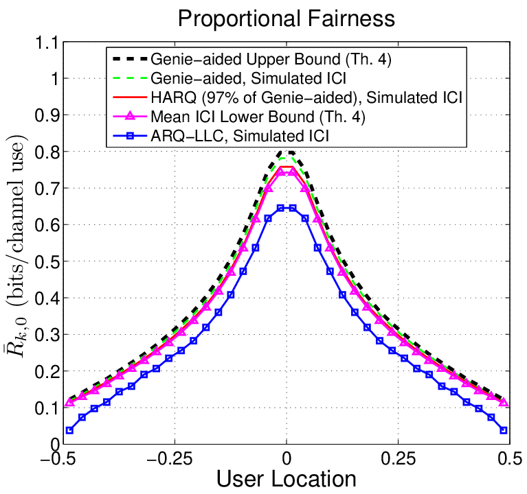
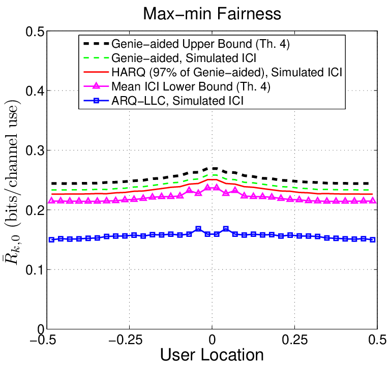
Figs. 2 and 3 compare user throughputs in cell under proportional fairness and max-min fairness, respectively. Thick dashed lines illustrate the throughput upper bounds of Theorem 4. Thin dashed lines correspond to the actual “genie-aided” rates achievable by the proposed HARQ scheme in the limit of infinite decoding delay. Solid lines show the throughput achieved by the HARQ scheme operating at finite average decoding delay for all users, by setting the parameters such that each user achieves 97% of the genie-aided rates (infinite delay). The “triangle” marks indicate the throughput lower bounds of Theorem 4. Finally, the “square” marks indicate the throughputs achieved by the conventional adaptive variable-rate coding with ARQ-LLC. We observe that under both fairness objective functions, the throughputs achieved by HARQ achieve a gain of more than 100% for the users at the edge of the cell in the proportional fairness case, and a throughput gain of more than 40% for all users in the max-min fairness case, with respect to the ARQ-LLC scheme.
Figs. 4 and 5 illustrate the average throughput as a function of the average decoding delay for the HARQ scheme in the case of two specific users: user at the left cell edge and at the cell center, under proportional fairness and max-min fairness, respectively. The thick dashed lines show genie-aided rates. The solid lines are obtained by increasing first-block coding rate parameter and computing average decoding delay from (25) with obtained by Monte Carlo simulation. Note that as increases, also the delay increases and the HARQ throughputs approach the genie-aided throughputs, in agreement with Theorem 3. The “o” marks indicate the throughput-delay points at which the HARQ protocol achieves 70%, 80% and 90% of the genie-aided throughput based on simulations. For example, under proportional fairness, 90% of the genie-aided throughput can be achieved at users and with average decoding delays of about and slots, respectively. These points (obtained by full system simulation) are accurately predicted by the analytical formulas of Section IV fitted with the Monte Carlo estimation of the probabilities .
For users per cell and BS antennas, assuming that exactly users are served in each slot, a round-robin scheduling with no outage (genie-aided rate allocation) would take an average delay of slots. Remarkably, under proportional fairness, 90% of the genie-aided throughput can be achieved with about slots of average delay for center user. This is only times that of the genie-aided round-robin scheduling. For edge users, this is achieved with slots of average delay for the edge users, which is only times that of round-robin. Under max-min fairness, both users and achieve genie-aided throughputs close to bits/channel use. The decoding delay for the center user is larger than for the edge user due to the fact that center users are scheduled very rarely. For the point, edge users achieve bits/channel use with average delay of slots while center users achieves a similar throughput of bits/channel use with delay of slots.
VI Concluding remarks
In this work we considered decentralized downlink scheduling in a multi-cell environment with multi-antenna BSs, where the scheduler at each BS has perfect CSIT about its own users and statistical information about the ICI caused by the other cells. Since each BS modifies its transmit covariance matrix at every slot, the ICI powers experienced at the users’ receivers are random variable. We addressed the scheduling problem in the presence of uncertain ICI powers in the framework of stochastic network optimization. A straightforward application of this framework yields a conventional scheme based on adaptive variable-rate coding at the physical layer, and ARQ at the Logical Link Control layer. Then, a new combination of the same stochastic network optimization framework with incremental redundancy Hybrid ARQ at the physical layer was shown to improve over the conventional scheme, and achieve a network utility arbitrarily close to the performance of a genie-aided system that can schedule the user rates equal to the (non-causally known) instantaneous mutual information on each slot. For this scheme, we also showed that all Nash equilibria of the multi-cell decentralized scheduling game yield network utility values that can be uniformly upper and lower bounded by virtual systems corresponding to “extremal” ICI statistics, where the lower bound corresponds to the case of deterministic ICI powers equal to their mean values, and the upper bound corresponds to the case where all interfering BSs transmit to a single user at full power (rank 1 interfering covariance matrices). These bounds stay at a fixed gap that is independent of the cellular system configuration, i.e., of the channel path gain coefficients and operating SNR. The proposed incremental redundancy HARQ can be implemented in practice by using Raptor codes [40] at the physical layer, and need no protocol overhead to communicate slot-by-slot rate allocation as in adaptive variable-rate coding. Hence, the proposed HARQ scheme is both easier to implement and performs significantly better than the conventional variable-rate coding scheme. Also, we hasten to say that our approach applies directly to a variety of possible configurations, including different MU-MIMO precoding schemes and network MIMO schemes with clusters of coordinated cells [46]. In this paper we considered the case of linear ZFBF and no cell clustering for the sake of clarity of exposition. The approach can also be extended to the case of non-perfect CSIT, following [18]. Here we focused on perfect CSIT for its simplicity and in order to focus on the random nature of ICI as the fundamental source of uncertainty in a multi-cell environment.
References
- [1] P. Bender, P. Black, M. Grob, R. Padovani, N. Sindhushayana, and A. Viterbi, “CDMA/HDR: A bandwidth-efficient high-speed wireless data service for nomadic users,” IEEE Commun. Mag., vol. 38, pp. 70–77, Jul. 2000.
- [2] A. Jalali, R. Padovani, and R. Pankaj, “Data throughput of CDMA-HDR: A high efficiency high data rate personal communication wireless system,” in Proc. IEEE Vehic. Tech. Conf., VTC-Spring, May 2000.
- [3] D. Tse, “Optimal power allocation over parallel Gaussian broadcast channels,” unpublished manuscript.
- [4] D. Tse and S. Hanly, “Multi-access fading channels: Part I: Polymatroid structure, optimal resource allocation and throughput capacities,” IEEE Trans. on Inform. Theory, vol. 44, no. 7, pp. 2796–2815, Nov. 1998.
- [5] P. Viswanath, D. N. C. Tse, and R. Laroia, “Opportunistic beamforming using dumb antennas,” IEEE Trans. on Inform. Theory, vol. 48, no. 6, pp. 1277–1294, Jun. 2002.
- [6] J. Mo and J. Walrand, “Fair end-to-end window-based congestion control,” IEEE/ACM Trans. Netw., vol. 8, no. 5, pp. 556–567, 2000.
- [7] http://www.3gpp.org/article/lte-advanced.
- [8] G. Caire and S. Shamai, “On the achievable throughput of a multiantenna Gaussian broadcast channel,” IEEE Trans. on Inform. Theory, vol. 49, no. 7, pp. 1691–1706, 2003.
- [9] H. Weingarten, Y. Steinberg, and S. Shamai, “The capacity region of the Gaussian multiple-input multiple-output broadcast channel,” IEEE Trans. on Inform. Theory, vol. 52, no. 9, pp. 3936–3964, Sep. 2006.
- [10] S. A. Ramprashad and G. Caire, “Cellular vs. network MIMO: A comparison including the channel state information overhead,” in Proc. IEEE Intern. Symp. on Personal, Indoor and Mobile Radio Commun., PIMRC, Tokyo, Japan, Sep. 2009.
- [11] G. Foschini, K. Karakayali, and R. A. Valenzuela, “Coordinating multiple antenna cellular networks to achieve enormous spectral efficiency,” IEE Proc. Commun., vol. 152, no. 4, pp. 548–555, Aug. 2006.
- [12] F. Boccardi, F. Tosato, and G. Caire, “Precoding Schemes for the MIMO-GBC,” in Proc. Int. Zurich Seminar on Commun., Feb. 2006, pp. 10–13.
- [13] T. Marzetta, “How Much Training is Required for Multiuser MIMO ?” Signals, Systems and Computers, 2006. ACSSC’06. Fortieth Asilomar Conference on, pp. 359–363, 2006.
- [14] G. Caire, N. Jindal, M. Kobayashi, and N. Ravindran, “Multiuser MIMO achievable rates with downlink training and channel state feedback,” submitted to IEEE Trans. on Inform. Theory, Nov. 2007, Arxiv preprint cs.IT/0711.2642v2.
- [15] P. Ding, D. Love, and M. Zoltowski, “Multiple antenna broadcast channels with shape feedback and limited feedback,” IEEE Trans. on Sig. Proc., vol. 55, no. 7, Part 1, pp. 3417–3428, Jul. 2007.
- [16] M. Kobayashi, G. Caire, and N. Jindal, “How much training and feedback are needed in MIMO broadcast channels?” in Proc. IEEE Int. Symp. on Inform. Theory, ISIT, Jul. 2008, pp. 2663–2667.
- [17] H. Shirani-Mehr and G. Caire, “Channel State Feedback Schemes for Multiuser MIMO-OFDM Downlink,” to appear in IEEE Trans. on Commun.
- [18] H. Shirani-Mehr, G. Caire, and M. J. Neely, “Mimo downlink scheduling with non-perfect channel state knowledge,” Submitted to IEEE Transactions on Communications.
- [19] L. Georgiadis, M. Neely, and L. Tassiulas, Resource Allocation and Cross-Layer Control in Wireless Networks, ser. Foundations and Trends in Networking. Hanover, MA, USA: Now Publishers Inc., 2006, vol. 1, no. 1.
- [20] G. Fodor and C. Koutsimanis, “A low intercell interference variation scheduler for ofdma networks,” in Communications, 2008. ICC ’08. IEEE International Conference on, May 2008, pp. 3078–3084.
- [21] M. T. Ivrlac and J. A. Nossek, “Intercell-interference in the gaussian miso broadcast channel,” in GLOBECOM. IEEE, 2007, pp. 3195–3199.
- [22] M. J. Neely, E. Modiano, and C. Li, “Fairness and optimal stochastic control for heterogeneous networks,” IEEE INFOCOM Proceedings, March 2005.
- [23] M. J. Neely, E. Modiano, and C. E. Rohrs, “Dynamic power allocation and routing for time varying wireless networks,” IEEE Journal on Selected Areas in Communications, Special Issue on Wireless Ad-Hoc Networks, vol. 23, no. 1, pp. 89 – 103, Jan 2005.
- [24] Q. Bi and S. Vitebsky, “Performance analysis of 3G-1X EVDO high data rate system,” in Proc. IEEE Wireless Commun. and Networking Conf., WCNC, vol. 1, Mar. 2002, pp. 389–395.
- [25] P. Frenger, S. Parkvall, and E. Dahlman, “Performance comparison of HARQ with Chase combining and incremental redundancy for HSDPA,” in Proc. IEEE Vehic. Tech. Conf, VTC-Fall, vol. 3, Sep. 2001, pp. 1829–1833.
- [26] R. Love, A. Ghosh, W. Xiao, and R. Ratasuk, “Performance of 3GPP high speed downlink packet access (HSDPA),” in Proc. IEEE Vehic. Tech. Conf., VTC-Fall, vol. 5, Sep. 2004, pp. 3359–3363.
- [27] G. Caire and D. Tuninetti, “The throughput of hybrid-ARQ protocols for the Gaussian collision channel,” IEEE Trans. on Inform. Theory, vol. 47, no. 5, pp. 1971–1988, Jul. 2001.
- [28] E. Biglieri, J. Proakis, and S. Shamai, “Fading channels: information-theoretic and communications aspects,” IEEE Trans. on Inform. Theory, vol. 44, no. 6, pp. 2619–2692, 1998.
- [29] A. Goldsmith, Wireless Communications. Cambridge University Press, 2005.
- [30] M. J. Neely, “Energy optimal control for time-varying wireless networks,” IEEE Transactions on Information Theory, vol. 52, no. 7, pp. 2915–2934, 2006.
- [31] J. Jose, A. Ashikhmin, P. Whiting, and S. Vishwanath, “Scheduling and pre-conditioning in multi-user MIMO TDD systems,” Arxiv preprint cs.IT/0709.4513.
- [32] P. Ding, D. Love, and M. Zoltowski, “Multiple Antenna Broadcast Channels With Shape Feedback and Limited Feedback,” IEEE Trans. on Sig. Proc., vol. 55, pp. 3417–3428, 2007.
- [33] J. W. Friedman, “A non-cooperative equilibrium for supergames,” Review of Economic Studies, vol. 38, no. 113, pp. 1–12, 1971. [Online]. Available: http://ideas.repec.org/a/bla/restud/v38y1971i113p1-12.html
- [34] ——, Oligopoly and the Theory of Games. Amsterdam [u.a.]: North-Holland, 1977.
- [35] J. B. Rosen, “Existence and uniqueness of equilibrium points for concave n-person games,” Econometrica, vol. 33, no. 3, pp. 520–534, 1965. [Online]. Available: http://dx.doi.org/10.2307/1911749
- [36] L. Ozarow, S. Shamai, and A. Wyner, “Information theoretic considerations for cellular mobile radio,” Vehicular Technology, IEEE Transactions on, vol. 43, no. 2, pp. 359–378, May 1994.
- [37] G. Dimic and N. Sidiropoulos, “On downlink beamforming with greedy user selection: performance analysis and simple new algorithm,” IEEE Trans. on Sig. Proc., vol. 53, no. 10, pp. 3857–3868, Oct. 2005.
- [38] T. Yoo and A. Goldsmith, “On the optimality of multiantenna broadcast scheduling using zero-forcing beamforming,” Selected Areas in Communications, IEEE Journal on, vol. 24, no. 3, pp. 528–541, March 2006.
- [39] H. Huh, H. Papadopoulos, and G. Caire, “MIMO broadcast channel optimization under general linear constraints,” in Information Theory, 2009. ISIT 2009. IEEE International Symposium on, 28 2009-July 3 2009, pp. 2664–2668.
- [40] A. Shokrollahi, “Raptor Codes,” IEEE Trans. on Inform. Theory, vol. 52, no. 6, pp. 2551–2567, Jun. 2006.
- [41] J. Forney, G., “Exponential error bounds for erasure, list, and decision feedback schemes,” Information Theory, IEEE Transactions on, vol. 14, no. 2, pp. 206–220, Mar 1968.
- [42] M. Sharif and B. Hassibi, “On the capacity of a mimo broadcast channel with partial side information,” IEEE Trans. on Inform. Theory, vol. 51, no. 2, pp. 506–522, Feb. 2005.
- [43] T. Yoo, N. Jindal, and A. Goldsmith, “Multi-Antenna Downlink Channels with Limited Feedback and User Selection,” IEEE J. Select. Areas Commun., vol. 25, pp. 1478–1491, 2007.
- [44] G. Grimmet and D. Stirzaker, Probability and Random Processes. Oxford Univ. Press, 2004.
- [45] M. Abramowitz and I. Stegun, Handbook of mathematical functions: with formulas, graphs, and mathematical tables. Courier Dover Publications, 1965.
- [46] G. Caire, S. A. Ramprashad, H. C. Papadopoulos, C. Pepin, and C.-E. W. Sundberg, “Multiuser MIMO downlink with limited inter-cell cooperation: Approximate interference alignment in time, frequency and space,” Proc. of Forty-Sixth Annual Allerton Conference on Communication, Control, and Computing, Sept. 2008.