跳到论文正文
W Papers独立论文阅读器 arXiv:1001.1151 论文正文 计算阅读时间 · 0%
引用这篇论文根据当前论文元数据生成,正式投稿前建议核对。


License: arXiv.org perpetual non-exclusive license
arXiv:1001.1151v1 [math-ph] 07 Jan 2010

Conformal field theory at central charge c=0c=0:
a measure of the indecomposability (bb) parameters.

Jérôme Dubail Affiliation: LPTENS, 24 rue Lhomond, 75231 Paris, France    Jesper Lykke Jacobsen Affiliation: LPTENS, 24 rue Lhomond, 75231 Paris, France    Hubert Saleur Affiliation: Department of Physics, University of Southern California, Los Angeles, CA 90089-0484    [2.0mm] Institut de Physique Théorique    CEA Saclay    91191 Gif Sur Yvette    France
Abstract

A good understanding of conformal field theory (CFT) at c=0c=0 is vital to the physics of disordered systems, as well as geometrical problems such as polymers and percolation. Steady progress has shown that these CFTs should be logarithmic, with indecomposable operator product expansions, and indecomposable representations of the Virasoro algebra. In one of the earliest papers on the subject, V. Gurarie introduced a single parameter bb to quantify this indecomposability in terms of the logarithmic partner tt of the stress energy tensor TT. He and A. Ludwig conjectured further that b=−58b=-\frac{5}{8} for polymers and b=56b=\frac{5}{6} for percolation. While a lot of physics may be hidden behind this parameter - which has also given rise to a lot of discussions - it had remained very elusive up to now, due to the lack of available methods to measure it experimentally or numerically, in contrast say with the central charge. We show in this paper how to overcome the many difficulties in trying to measure bb. This requires control of a lattice scalar product, lattice Jordan cells, together with a precise construction of the state L−2​|0⟩L_{-2}|0\rangle. The final result is that b=56b=\frac{5}{6} for polymers. For percolation, we find that b=−58b=-\frac{5}{8} within an XXZ or supersymmetric representation. In the geometrical representation, we do not find a Jordan cell for L0L_{0} at level two (finite-size Hamiltonian and transfer matrices are fully diagonalizable), so there is no bb in this case.

Introduction

In the last twenty years or so since the seminal paper [1] of Belavin, Polyakov and Zamolodchikov, Conformal Field Theory (CFT) has proven amazingly successful. It is now an essential item in the toolbox of condensed matter and string theorists, and has had a profound impact on several sub-fields of modern mathematics.

Yet, despite this flurry of successes, some very fundamental questions have remained unanswered to this day. One of these questions concerns percolation, the very geometrical critical problem where CFT has obtained some of its most impressive results. In a nutshell, despite years of work and some progress (see below), we do not know any conformal field theory describing at least some of the geometrical observables (be it hulls, clusters or backbones) in a fully consistent way. As a result, many quantities involving bulk correlations functions—for instance the equivalent of the Binder cumulant [2] in this problem [3]—are, to this day, unknown analytically.

Another vexing question concerns the celebrated transition between plateaux in the integer quantum Hall effect. The evidence is strong that it corresponds to quantum critical points of the 2+1 dimensional electron gas. The physics of the transition is somewhat well understood (and involves an interplay between disorder, which tends to localize the electrons, and the kinetic energy, quenched by the strong magnetic field, which causes delocalization), and qualitatively well described by a 2D sigma model with topological term [4]. Nevertheless, a precise identification of the low energy effective field theory is still lacking to this day, despite the wealth of theoretical and numerical works on the topic, and the fact that this theory is expected to be conformally invariant (see [5] for an insightful review).

The origin of these difficulties is, ultimately, the fact that the CFTs describing these problems have to be non unitary, with vanishing central charge. Non-unitarity in a CFT can have rather mild consequences—like in the minimal theories such as the Yang Lee edge singularity. It took a while to realize that non-unitarity would most often (in particular, when c=0c=0) imply in fact indecomposability, leading to a very difficult kind of theory called a logarithmic CFT (LCFT).

LCFTs were probably first encountered in published form in a paper by Rozansky and Saleur [6]. In this paper, the authors studied a particular kind of c=0c=0 theory with U⁡(1|1)U(1|1) supergroup symmetry, and stumbled upon four-point functions involving logarithmic dependence on the cross ratio. These authors correctly related this property to the indecomposability of the operator product expansions (OPE), and to the non-diagonalizability of the L0L_{0} generator, inherited from the non semi-simplicity of the symmetry algebra. Shortly after, Gurarie [7] pointed out that these features were in fact necessary to have a consistent, non-trivial CFT at c=0c=0. Later, Gurarie [8] and Gurarie and Ludwig [9] built up a very attractive formalism within which CFTs at c=0c=0 must possess, in addition to their stress energy tensor T⁡(z)T(z), an extra field whose holomorphic part, t⁡(z)t(z), has conformal weight two. The singular part of the OPE between T⁡(z)T(z) and t⁡(z)t(z) is determined up to a new universal number, an “anomaly” usually denoted by bb. This parameter is expected in [8, 9] to play a very important physical role. It might obey a “c-theorem” [7] and thus indicate possible directions of RG flows within theories with vanishing central charge. Its value also dictates the existence of null vectors for conformal weights contained in the Kac table, and is thus profoundly related with the determination of four-point functions. Gurarie and Ludwig [9] suggested, based on knowledge of critical exponents from Coulomb gas calculations and some heuristic hypotheses, that b=−58b=-\frac{5}{8} for polymers and b=56b=\frac{5}{6} for percolation.11 1 We shall define bb precisely below.

Despite the appeal of the ideas proposed in [8, 9], only very little progress has happened to make them into a powerful theoretical tool. It is not clear for instance to what extent it is possible or helpful to study further the extension of the Virasoro algebra proposed in [9]. Considerable difficulties also arise when one tries to build non-chiral theories by combining the left and right moving sectors. Most examples worked out so far indeed concern only boundary LCFTs.

Meanwhile, the subject has matured with the understanding that, probably, rather than a single parameter bb, LCFTs might be characterized by a complicated structure of indecomposable Virasoro modules. This structure involves maps between sub-modules, and several parameters to describe their precise action. This line of thought shows how close the problem is to the theory of non semi-simple Lie (super)algebras, whose representation theory is more often than not of the “wild” type. Progress has been steady in trying to understand indecomposable Virasoro modules [10, 11, 12, 13, 14] in general LCFTs. For c=0c=0 the bb parameters appear indeed as some particular coefficient describing the embedding of a sub-module. Some simple algebraic arguments suggest then that b=−58b=-\frac{5}{8} for percolation and b=56b=\frac{5}{6} for polymers, that is, the value of Gurarie and Ludwig [9] up to a switch.

In the last two years, more progress has occurred from the direction of lattice models. It had long been known that the representation theory of lattice algebras (mostly, the Temperley-Lieb algebra) bore some striking resemblance to that of the Virasoro algebra. In particular, it had been known that when qq is a root of unity, the hamiltonian (the lattice discretization of L0L_{0}, or L0+L¯0L_{0}+\bar{L}_{0} depending on the boundary conditions) can sometimes be non-diagonalizable, and that Jordan cells appear, very much mimicking the ones expected in the continuum limit. This was explored in a much more systematic fashion in works by Pearce, Rasmussen and Zuber [15, 16, 17] and independently by Read and Saleur [18]. The outcome of these analyses was a rather coherent picture of the indecomposable Virasoro modules appearing in some families of boundary LCFTs, including percolation and polymers, together with some formal but potentially useful results about fusion. This picture was interpreted in interesting mathematical terms in [19].

Yet, large parts of these constructions are still speculative. For instance, the lattice analysis clearly shows which modules are mapped into each other under the action of the lattice algebras, but what this becomes precisely in the continuum limit—including which Virasoro generators and states are involved in these mappings, together with precise values of the corresponding coefficients—is largely conjectural. Moreover, it is clear that only the ‘simplest indecomposable’ modules have been encountered so far, and one is still far from being able to guess what would happen, say, for the quantum Hall plateau transition.

One of the crucial remaining obstacles is that the features that make LCFTs difficult are also very hard to observe or measure directly. It is quite striking for instance, that despite the 15 year old controversy around the value of the bb parameter for percolation or polymers—problems which are usually rather easy to study numerically—no way to measure this parameter has been available, up to now. One of the only forays in this direction is the paper by Koo and Saleur [20], who attempted to define and study a straightforward regularization of the Virasoro algebra on the lattice. Their success was only partial, and hampered by the fact that the continuum limit of commutators is not the commutator of the continuum limits.

We shall report in this paper a method to measure the parameter bb in lattice models. While it might not be general enough to work for all theories at c=0c=0, it certainly will allow us to assert what the values of this parameter for percolation and polymers actually are.

The paper is organized as follows. In the first section, we recall basic facts about the bb number in LCFTs at c=0c=0, and define a general strategy to measure it. This strategy requires overcoming two difficulties. One is finding a scalar product on the lattice that goes to the Virasoro-Shapovalov form in the continuum limit. The other is finding a regularization of the L−2L_{-2} operator—or more precisely, of its action on the vacuum. These difficulties are solved in the next two sections. In section 4, we finally gather all the pieces to study the Jordan cells for percolation and polymers, and measure bb.

1 The bb number

In a nutshell, the argument of Gurarie [7, 8, 9] went as follows. Conformal invariance fixes the coefficient of the stress tensor TT in the OPE of an operator with itself (assuming there is a single field with h=2,h¯=0h=2,\bar{h}=0) to be of the form

ϕ⁡(z)​ϕ​(0)≈aϕ​z−2​hϕ​(1+2​hϕc​T​(z)+…)\phi(z)\phi(0)\approx a_{\phi}z^{-2h_{\phi}}\left(1+\frac{2h_{\phi}}{c}T(z)+\ldots\right) (1)

Here aϕa_{\phi} is an amplitude, determining the normalization of the two-point function

⟨ϕ⁡(z,z¯)​ϕ​(0,0)⟩=|aϕ|2​1z2​hϕ​z¯2​h¯ϕ\langle\phi(z,\bar{z})\phi(0,0)\rangle=|a_{\phi}|^{2}\frac{1}{z^{2h_{\phi}}\bar{z}^{2\bar{h}_{\phi}}} (2)

If one want to keep aϕa_{\phi} finite in a theory at c=0c=0 for an operator with hϕ≠0h_{\phi}\neq 0, the 2​hϕc\frac{2h_{\phi}}{c} factor poses problems as it diverges.

There are various ways to resolve the difficulty (this was also discussed in [21, 22]. First, a divergence in the OPE coefficient (which would manifest itself in a physical quantity such as a four point function) might not be a problem after all, but have a physical meaning, related with some n→0n\to 0 limit. Second, it could be that demanding aϕa_{\phi} finite is not physically meaningful, again in relation with an n→0n\to 0 limit. Recall that since we are dealing with non-unitary theories, having a vanishing two-point function does not mean that the corresponding operator is zero. The third way to resolve the difficulty is to admit that there are other operators with h=2h=2 appearing on the right-hand side of the OPE (1). These operators might be part of a supersymmetry multiplet, such as those that might occur in supergroup WZW models [23] and other supersymmetric CFTs [24]. We note that in such cases, there is no need for a logarithmic dependence in the OPE at this order, although the theory will in general be logarithmic (see, e.g., [23]. The other scenario proposed in [9] is of an n→0n\to 0 limit, with another operator whose dimension is generically different from 2 becoming degenerate with TT. In this case—examples of which can be worked out in details for the models with central charge c=1−6x⁡(x+1)c=1-\frac{6}{x(x+1)}, in the limit x→2x\to 2—one expects the OPE of ϕ\phi with itself to read instead

ϕ⁡(z)​ϕ​(0)≈aϕ​z−2​hϕ​(1+2​hϕb​z2​[t⁡(0)+log⁡(z)​T​(0)]+…).\phi(z)\phi(0)\approx a_{\phi}z^{-2h_{\phi}}\left(1+\frac{2h_{\phi}}{b}z^{2}[t(0)+\log(z)T(0)]+\ldots\right)\,. (3)

The operator tt is called ‘logarithmic partner’ of TT, and forms with it a logarithmic pair, that is, a set of fields on which the L0L_{0} operator is not diagonalizable but has the form of a Jordan cell

L0​|T⟩=2​|T⟩,L0​|t⟩=2​|t⟩+|T⟩L_{0}|T\rangle=2|T\rangle,\penalty\ \penalty\ \penalty\ L_{0}|t\rangle=2|t\rangle+|T\rangle (4)

In terms of two-point functions one has

⟨T⁡(z)​T​(0)⟩\displaystyle\langle T(z)T(0)\rangle =\displaystyle= 0\displaystyle 0 (5a)
⟨T⁡(z)​t​(0)⟩\displaystyle\langle T(z)t(0)\rangle =\displaystyle= bz4\displaystyle\frac{b}{z^{4}} (5b)
⟨t⁡(z)​t​(0)⟩\displaystyle\langle t(z)t(0)\rangle =\displaystyle= −2​b​log⁡z+az4\displaystyle\frac{-2b\log z+a}{z^{4}} (5c)

where the last result comes from imposing global conformal invariance [9]. Note that the normalization of TT is crucial in defining the numerical value of bb, once a choice has been made that the L0L_{0} Jordan cell has off-diagonal term unity (which translates into the relative normalization of the last two equations). There remains, on the other hand, a choice t→t+constant ​Tt\to t+\hbox{constant }T, which does not affect the leading terms in the OPE, but only the constant aa.

The universality of these OPEs, the value of the number bb and its properties (e.g., under RG flows) have all been subject of intense debate. It is not our purpose to review this debate in detail. We only wish to recall that, when thinking of the limit of minimal models as c→0c\to 0, one is naturally led to two candidates which might become degenerate with TT: the (3,1)(3,1) field and the (1,5)(1,5) field (in Kac table notations). The former choice leads to b=56b=\frac{5}{6}, and the latter to b=−58b=-\frac{5}{8}. Using a variety of arguments, Gurarie and Ludwig [9] predicted that the former choice corresponds to percolation, and the latter to polymers, which are therefore profoundly different logarithmic CFTs.

While one can dwell at great length on the merits of the arguments in [9] we believe it is more constructive to ask whether one can, in fact, measure the parameter bb. Some considerable difficulties arise when thinking of this possibility. One might, of course, try to identify tt in a lattice model of percolation or polymers. After all, it is quite possible to get a handle on the meaning of TT itself [25, 26]. But measuring directly correlation functions such as those in (5) is a very daunting task, not to mention the difficulty of extracting properly a logarithmic dependence. We also note that the formalism in [9] is really a chiral one, where the job of glueing back together the left and right parts of the theory is left for further work, and might lead to considerable surprises. This chiral aspect naturally suggests turning to the physics of the boundary theory, which is in fact what is mostly considered in [9].

Short of measuring correlation functions on the lattice, the next best hope would be to access numerically bb through a lattice analog of the Jordan cell structure in (4). Some progress in reproducing algebraic relations—e.g., the Virasoro commutation relations—in lattice models was reported in fact in [20], and it is a natural idea to try to push further the results obtained there. Introduce first the scalar product and the notion of adjoint from in and out states as usual [27], with Ln†=L−nL_{n}^{\dagger}=L_{-n} (of course now the form is not positive definite). Then the relations equivalent to (5) are

L0=(2102)L_{0}=\left(\begin{array}[]{cc}2&1\\ 0&2\end{array}\right) (6)

in the basis {T,t}\{T,t\}, where

|T⟩=L−2​|0⟩\displaystyle|T\rangle=L_{-2}|0\rangle , ⟨T|T⟩=0\displaystyle\langle T|T\rangle=0
L2​|t⟩=b​|0⟩\displaystyle L_{2}|t\rangle=b|0\rangle , ⟨t|T⟩=b.\displaystyle\langle t|T\rangle=b\,. (7)

We see that a possible strategy to measure bb would involve finding a Jordan cell for the hamiltonian (the lattice version of L0L_{0}) in finite size. One would then have to identify the states corresponding to T,tT,t and normalize them properly. Finally one would have to calculate the scalar product ⟨t|T⟩\langle t|T\rangle. We shall accomplish this program here, but first let us stress why it is difficult, and has not been done before.

The first obstacle is to find a Jordan cell in lattice models. This in fact is quite easy, as has been known for a while. The point is that the ‘hamiltonians’ in lattice models whose continuum limit is a CFT are often non-diagonalizable, a consequence of their deep relationship with lattice symmetries (quantum groups) or lattice algebras (Temperley-Lieb algebras) which have non semi-simplicity properties fully emulating those of the continuum limit. Nevertheless, the question whether there exists a Jordan cell for L0L_{0} in a given lattice model is not easily answered a priori—we shall mention some surprises along these lines later.

Having obtained the Jordan cell, one needs to identify TT. While it is natural to think that TT is an eigenvector of the hamiltonian, a very important obstacle is its normalization. While crucial to determine the value of bb, it cannot be done via a standard eigenvector normalization since the two-point function of TT vanishes in the continuum, which manifests itself by the fact that |T⟩|T\rangle—or rather its lattice equivalent—is a null state. To normalize TT, we shall resort to a very indirect trick that we call the “trousers trick”, which is really at the heart of our solution of the problem.

Finally, one needs to properly normalize tt via the desired Jordan cell structure. This is quite involved with big transfer matrices, and requires some numerical tricks. We note in passing that, according to (5​c\ref{corrf}\,c), |t⟩|t\rangle turns out to have infinite norm square.

2 Lattice scalar products

2.1 Hamiltonians and Transfer Matrices

A 2D classical statistical model can be viewed as a 1+1D model evolving in imaginary time. At large length scales, the low-energy excitations of the latter are described by some quantum field theory. When the 2D model is at a critical point, these excitations are gapless, hence the field theory becomes conformal. A 1+1D system of width LL is defined by its Hamiltonian HLH_{L}, or by its transfer matrix TLT_{L} when it comes from a 2D statistical model.

Let us start by considering the Ising model as an example. The critical Ising chain is defined by the Hamiltonian (say with periodic boundary conditions σL+1z=σ1z\sigma^{z}_{L+1}=\sigma^{z}_{1})

HL=−∑i=1Lσizσi+1z−∑i=1LσixH_{L}=-\sum_{i=1}^{L}\sigma_{i}^{z}\sigma_{i+1}^{z}-\sum_{i=1}^{L}\sigma_{i}^{x} (8)

acting on the space of spin configurations |↑↓↓↑…↓⟩\left|\uparrow\downarrow\downarrow\uparrow\dots\downarrow\right>. HLH_{L} is hermitian, therefore in the continuum limit is described by a unitary CFT. It is well-known that it corresponds to the minimal model ℳ4,3\mathcal{M}_{4,3} with central charge c=1/2c=1/2.

Now, our second example will turn out to be non-unitary. It is a dense loop model, given by the transfer matrix (in the picture L=6L=6)

TL=T_{L}\;= (9)

where each square is a sum over two terms

++≡\equiv

and one takes periodic boundary conditions (dotted lines are identified). Iterations of TLT_{L} (from bottom to top) build the partition function of the dense loop model on a cylinder.

We have not specified yet on which configuration space TLT_{L} is acting. Here the basis states will encode the planar pairings of LL points, such as |              ⟩\left|\;\hbox to29.25pt{\vbox to7.91pt{\pgfpicture\makeatletter\hbox{\hskip 0.4pt\lower-7.51318pt\hbox to0.0pt{\lxSVG@begingroup@{_scopebegin=1} \lxSVG@begingroup@{stroke=#000000} \lxSVG@begingroup@{fill=#000000} \lxSVG@setlinewidth{\the\pgflinewidth}\lxSVG@begingroup@{stroke-width=0.4pt} \lx@inpgf@ignorespaces\nullfont\hbox to0.0pt{\lxSVG@begingroup@{_scopebegin=1} {}{{}}{}{{}{}{\lx@inpgf@ignorespaces}{{\lx@inpgf@ignorespaces}}{{{{}{}{}{}}} {{}{}{}{}}}}{} {} {} {} {}{}\lxSVG@begingroup@{_scopebegin=1} \lxSVG@setlinewidth{\the\pgflinewidth}\lxSVG@begingroup@{stroke-width=0.8pt} \lx@inpgf@ignorespaces{}\lxSVG@stroke\lxSVG@drawpath@unclipped{M 0 0 C 0 -5.44 1.76 -9.84 3.94 -9.84 C 6.11 -9.84 7.87 -5.44 7.87 0}{fill:none} \lx@inpgf@ignorespaces \lxSVG@closescope {}{{}}{}{{}{}{\lx@inpgf@ignorespaces}{{\lx@inpgf@ignorespaces}}{{{{}{}{}{}}} {{}{}{}{}}}}{} {} {} {} {}{}\lxSVG@begingroup@{_scopebegin=1} \lxSVG@setlinewidth{\the\pgflinewidth}\lxSVG@begingroup@{stroke-width=0.8pt} \lx@inpgf@ignorespaces{}\lxSVG@stroke\lxSVG@drawpath@unclipped{M 15.75 0 C 15.75 -5.44 21.04 -9.84 27.56 -9.84 C 34.08 -9.84 39.37 -5.44 39.37 0}{fill:none} \lx@inpgf@ignorespaces \lxSVG@closescope {}{{}}{}{{}{}{\lx@inpgf@ignorespaces}{{\lx@inpgf@ignorespaces}}{{{{}{}{}{}}} {{}{}{}{}}}}{} {} {} {} {}{}\lxSVG@begingroup@{_scopebegin=1} \lxSVG@setlinewidth{\the\pgflinewidth}\lxSVG@begingroup@{stroke-width=0.8pt} \lx@inpgf@ignorespaces{}\lxSVG@stroke\lxSVG@drawpath@unclipped{M 23.62 0 C 23.62 -3.26 25.39 -5.91 27.56 -5.91 C 29.73 -5.91 31.5 -3.26 31.5 0}{fill:none} \lx@inpgf@ignorespaces \lxSVG@closescope \lxSVG@closescope {\lx@inpgf@ignorespaces}{\lx@inpgf@ignorespaces}{\lx@inpgf@ignorespaces}\hss}\lxSVG@discardpath\lxSVG@closescope \hss}}\lxSVG@closescope\endpgfpicture}}\;\right> or |              ⟩\left|\;\hbox to29.25pt{\vbox to7.91pt{\pgfpicture\makeatletter\hbox{\hskip 0.4pt\lower-7.51318pt\hbox to0.0pt{\lxSVG@begingroup@{_scopebegin=1} \lxSVG@begingroup@{stroke=#000000} \lxSVG@begingroup@{fill=#000000} \lxSVG@setlinewidth{\the\pgflinewidth}\lxSVG@begingroup@{stroke-width=0.4pt} \lx@inpgf@ignorespaces\nullfont\hbox to0.0pt{\lxSVG@begingroup@{_scopebegin=1} {}{{}}{}{{}{}{\lx@inpgf@ignorespaces}{{\lx@inpgf@ignorespaces}}{{{{}{}{}{}}} {{}{}{}{}}}}{} {} {} {} {}{}\lxSVG@begingroup@{_scopebegin=1} \lxSVG@setlinewidth{\the\pgflinewidth}\lxSVG@begingroup@{stroke-width=0.8pt} \lx@inpgf@ignorespaces{}\lxSVG@stroke\lxSVG@drawpath@unclipped{M 0 0 C 0 -5.44 8.81 -9.84 19.69 -9.84 C 30.56 -9.84 39.37 -5.44 39.37 0}{fill:none} \lx@inpgf@ignorespaces \lxSVG@closescope {}{{}}{}{{}{}{\lx@inpgf@ignorespaces}{{\lx@inpgf@ignorespaces}}{{{{}{}{}{}}} {{}{}{}{}}}}{} {} {} {} {}{}\lxSVG@begingroup@{_scopebegin=1} \lxSVG@setlinewidth{\the\pgflinewidth}\lxSVG@begingroup@{stroke-width=0.8pt} \lx@inpgf@ignorespaces{}\lxSVG@stroke\lxSVG@drawpath@unclipped{M 7.87 0 C 7.87 -3.26 9.64 -5.91 11.81 -5.91 C 13.99 -5.91 15.75 -3.26 15.75 0}{fill:none} \lx@inpgf@ignorespaces \lxSVG@closescope {}{{}}{}{{}{}{\lx@inpgf@ignorespaces}{{\lx@inpgf@ignorespaces}}{{{{}{}{}{}}} {{}{}{}{}}}}{} {} {} {} {}{}\lxSVG@begingroup@{_scopebegin=1} \lxSVG@setlinewidth{\the\pgflinewidth}\lxSVG@begingroup@{stroke-width=0.8pt} \lx@inpgf@ignorespaces{}\lxSVG@stroke\lxSVG@drawpath@unclipped{M 23.62 0 C 23.62 -3.26 25.39 -5.91 27.56 -5.91 C 29.73 -5.91 31.5 -3.26 31.5 0}{fill:none} \lx@inpgf@ignorespaces \lxSVG@closescope \lxSVG@closescope {\lx@inpgf@ignorespaces}{\lx@inpgf@ignorespaces}{\lx@inpgf@ignorespaces}\hss}\lxSVG@discardpath\lxSVG@closescope \hss}}\lxSVG@closescope\endpgfpicture}}\;\right> for L=6L=6. A state in this model is a linear combination of such basis states. The action of TLT_{L} on basis states is found by stacking the diagrams from bottom to top, e.g.:

|              ⟩=\left|\;\hbox to29.25pt{\vbox to7.91pt{\pgfpicture\makeatletter\hbox{\hskip 0.4pt\lower-7.51318pt\hbox to0.0pt{\lxSVG@begingroup@{_scopebegin=1} \lxSVG@begingroup@{stroke=#000000} \lxSVG@begingroup@{fill=#000000} \lxSVG@setlinewidth{\the\pgflinewidth}\lxSVG@begingroup@{stroke-width=0.4pt} \lx@inpgf@ignorespaces\nullfont\hbox to0.0pt{\lxSVG@begingroup@{_scopebegin=1} {}{{}}{}{{}{}{\lx@inpgf@ignorespaces}{{\lx@inpgf@ignorespaces}}{{{{}{}{}{}}} {{}{}{}{}}}}{} {} {} {} {}{}\lxSVG@begingroup@{_scopebegin=1} \lxSVG@setlinewidth{\the\pgflinewidth}\lxSVG@begingroup@{stroke-width=0.8pt} \lx@inpgf@ignorespaces{}\lxSVG@stroke\lxSVG@drawpath@unclipped{M 0 0 C 0 -5.44 1.76 -9.84 3.94 -9.84 C 6.11 -9.84 7.87 -5.44 7.87 0}{fill:none} \lx@inpgf@ignorespaces \lxSVG@closescope {}{{}}{}{{}{}{\lx@inpgf@ignorespaces}{{\lx@inpgf@ignorespaces}}{{{{}{}{}{}}} {{}{}{}{}}}}{} {} {} {} {}{}\lxSVG@begingroup@{_scopebegin=1} \lxSVG@setlinewidth{\the\pgflinewidth}\lxSVG@begingroup@{stroke-width=0.8pt} \lx@inpgf@ignorespaces{}\lxSVG@stroke\lxSVG@drawpath@unclipped{M 15.75 0 C 15.75 -5.44 21.04 -9.84 27.56 -9.84 C 34.08 -9.84 39.37 -5.44 39.37 0}{fill:none} \lx@inpgf@ignorespaces \lxSVG@closescope {}{{}}{}{{}{}{\lx@inpgf@ignorespaces}{{\lx@inpgf@ignorespaces}}{{{{}{}{}{}}} {{}{}{}{}}}}{} {} {} {} {}{}\lxSVG@begingroup@{_scopebegin=1} \lxSVG@setlinewidth{\the\pgflinewidth}\lxSVG@begingroup@{stroke-width=0.8pt} \lx@inpgf@ignorespaces{}\lxSVG@stroke\lxSVG@drawpath@unclipped{M 23.62 0 C 23.62 -3.26 25.39 -5.91 27.56 -5.91 C 29.73 -5.91 31.5 -3.26 31.5 0}{fill:none} \lx@inpgf@ignorespaces \lxSVG@closescope \lxSVG@closescope {\lx@inpgf@ignorespaces}{\lx@inpgf@ignorespaces}{\lx@inpgf@ignorespaces}\hss}\lxSVG@discardpath\lxSVG@closescope \hss}}\lxSVG@closescope\endpgfpicture}}\;\right>==|              ⟩=\left|\;\hbox to29.25pt{\vbox to7.91pt{\pgfpicture\makeatletter\hbox{\hskip 0.4pt\lower-7.51318pt\hbox to0.0pt{\lxSVG@begingroup@{_scopebegin=1} \lxSVG@begingroup@{stroke=#000000} \lxSVG@begingroup@{fill=#000000} \lxSVG@setlinewidth{\the\pgflinewidth}\lxSVG@begingroup@{stroke-width=0.4pt} \lx@inpgf@ignorespaces\nullfont\hbox to0.0pt{\lxSVG@begingroup@{_scopebegin=1} {}{{}}{}{{}{}{\lx@inpgf@ignorespaces}{{\lx@inpgf@ignorespaces}}{{{{}{}{}{}}} {{}{}{}{}}}}{} {} {} {} {}{}\lxSVG@begingroup@{_scopebegin=1} \lxSVG@setlinewidth{\the\pgflinewidth}\lxSVG@begingroup@{stroke-width=0.8pt} \lx@inpgf@ignorespaces{}\lxSVG@stroke\lxSVG@drawpath@unclipped{M 0 0 C 0 -5.44 5.29 -9.84 11.81 -9.84 C 18.33 -9.84 23.62 -5.44 23.62 0}{fill:none} \lx@inpgf@ignorespaces \lxSVG@closescope {}{{}}{}{{}{}{\lx@inpgf@ignorespaces}{{\lx@inpgf@ignorespaces}}{{{{}{}{}{}}} {{}{}{}{}}}}{} {} {} {} {}{}\lxSVG@begingroup@{_scopebegin=1} \lxSVG@setlinewidth{\the\pgflinewidth}\lxSVG@begingroup@{stroke-width=0.8pt} \lx@inpgf@ignorespaces{}\lxSVG@stroke\lxSVG@drawpath@unclipped{M 7.87 0 C 7.87 -3.26 9.64 -5.91 11.81 -5.91 C 13.99 -5.91 15.75 -3.26 15.75 0}{fill:none} \lx@inpgf@ignorespaces \lxSVG@closescope {}{{}}{}{{}{}{\lx@inpgf@ignorespaces}{{\lx@inpgf@ignorespaces}}{{{{}{}{}{}}} {{}{}{}{}}}}{} {} {} {} {}{}\lxSVG@begingroup@{_scopebegin=1} \lxSVG@setlinewidth{\the\pgflinewidth}\lxSVG@begingroup@{stroke-width=0.8pt} \lx@inpgf@ignorespaces{}\lxSVG@stroke\lxSVG@drawpath@unclipped{M 31.5 0 C 31.5 -5.44 33.26 -9.84 35.43 -9.84 C 37.61 -9.84 39.37 -5.44 39.37 0}{fill:none} \lx@inpgf@ignorespaces \lxSVG@closescope \lxSVG@closescope {\lx@inpgf@ignorespaces}{\lx@inpgf@ignorespaces}{\lx@inpgf@ignorespaces}\hss}\lxSVG@discardpath\lxSVG@closescope \hss}}\lxSVG@closescope\endpgfpicture}}\;\right>

Each closed loop gets a Boltzmann weight nn. For our formalism to be complete, we need to define a transposition operation (or equivalently a scalar product).

2.2 Transposition and scalar product

How can we define the forms ⟨.|\left<.\right| ? In our geometrical formulation, the elements of the transfer matrix should act on such an object from top to bottom:

⟨              |\left<{\;\hbox to29.25pt{\vbox to7.91pt{\pgfpicture\makeatletter\hbox{\hskip 0.4pt\lower-0.4pt\hbox to0.0pt{\lxSVG@begingroup@{_scopebegin=1} \lxSVG@begingroup@{stroke=#000000} \lxSVG@begingroup@{fill=#000000} \lxSVG@setlinewidth{\the\pgflinewidth}\lxSVG@begingroup@{stroke-width=0.4pt} \lx@inpgf@ignorespaces\nullfont\hbox to0.0pt{\lxSVG@begingroup@{_scopebegin=1} {}{{}}{}{{}{}{\lx@inpgf@ignorespaces}{{\lx@inpgf@ignorespaces}}{{{{}{}{}{}}}{{}{}{}{}}}}{} {} {} {} {}{}\lxSVG@begingroup@{_scopebegin=1} \lxSVG@setlinewidth{\the\pgflinewidth}\lxSVG@begingroup@{stroke-width=0.8pt} \lx@inpgf@ignorespaces{}\lxSVG@stroke\lxSVG@drawpath@unclipped{M 0 0 C 0 5.44 5.29 9.84 11.81 9.84 C 18.33 9.84 23.62 5.44 23.62 0}{fill:none} \lx@inpgf@ignorespaces \lxSVG@closescope {}{{}}{}{{}{}{\lx@inpgf@ignorespaces}{{\lx@inpgf@ignorespaces}}{{{{}{}{}{}}}{{}{}{}{}}}}{} {} {} {} {}{}\lxSVG@begingroup@{_scopebegin=1} \lxSVG@setlinewidth{\the\pgflinewidth}\lxSVG@begingroup@{stroke-width=0.8pt} \lx@inpgf@ignorespaces{}\lxSVG@stroke\lxSVG@drawpath@unclipped{M 7.87 0 C 7.87 3.26 9.64 5.91 11.81 5.91 C 13.99 5.91 15.75 3.26 15.75 0}{fill:none} \lx@inpgf@ignorespaces \lxSVG@closescope {}{{}}{}{{}{}{\lx@inpgf@ignorespaces}{{\lx@inpgf@ignorespaces}}{{{{}{}{}{}}}{{}{}{}{}}}}{} {} {} {} {}{}\lxSVG@begingroup@{_scopebegin=1} \lxSVG@setlinewidth{\the\pgflinewidth}\lxSVG@begingroup@{stroke-width=0.8pt} \lx@inpgf@ignorespaces{}\lxSVG@stroke\lxSVG@drawpath@unclipped{M 31.5 0 C 31.5 5.44 33.26 9.84 35.43 9.84 C 37.61 9.84 39.37 5.44 39.37 0}{fill:none} \lx@inpgf@ignorespaces \lxSVG@closescope \lxSVG@closescope {\lx@inpgf@ignorespaces}{\lx@inpgf@ignorespaces}{\lx@inpgf@ignorespaces}\hss}\lxSVG@discardpath\lxSVG@closescope \hss}}\lxSVG@closescope\endpgfpicture}}}\;\right|===n⟨              |=\;n\;\left<{\;\hbox to29.25pt{\vbox to7.91pt{\pgfpicture\makeatletter\hbox{\hskip 0.4pt\lower-0.4pt\hbox to0.0pt{\lxSVG@begingroup@{_scopebegin=1} \lxSVG@begingroup@{stroke=#000000} \lxSVG@begingroup@{fill=#000000} \lxSVG@setlinewidth{\the\pgflinewidth}\lxSVG@begingroup@{stroke-width=0.4pt} \lx@inpgf@ignorespaces\nullfont\hbox to0.0pt{\lxSVG@begingroup@{_scopebegin=1} {}{{}}{}{{}{}{\lx@inpgf@ignorespaces}{{\lx@inpgf@ignorespaces}}{{{{}{}{}{}}}{{}{}{}{}}}}{} {} {} {} {}{}\lxSVG@begingroup@{_scopebegin=1} \lxSVG@setlinewidth{\the\pgflinewidth}\lxSVG@begingroup@{stroke-width=0.8pt} \lx@inpgf@ignorespaces{}\lxSVG@stroke\lxSVG@drawpath@unclipped{M 0 0 C 0 5.44 1.76 9.84 3.94 9.84 C 6.11 9.84 7.87 5.44 7.87 0}{fill:none} \lx@inpgf@ignorespaces \lxSVG@closescope {}{{}}{}{{}{}{\lx@inpgf@ignorespaces}{{\lx@inpgf@ignorespaces}}{{{{}{}{}{}}}{{}{}{}{}}}}{} {} {} {} {}{}\lxSVG@begingroup@{_scopebegin=1} \lxSVG@setlinewidth{\the\pgflinewidth}\lxSVG@begingroup@{stroke-width=0.8pt} \lx@inpgf@ignorespaces{}\lxSVG@stroke\lxSVG@drawpath@unclipped{M 15.75 0 C 15.75 5.44 17.51 9.84 19.69 9.84 C 21.86 9.84 23.62 5.44 23.62 0}{fill:none} \lx@inpgf@ignorespaces \lxSVG@closescope {}{{}}{}{{}{}{\lx@inpgf@ignorespaces}{{\lx@inpgf@ignorespaces}}{{{{}{}{}{}}}{{}{}{}{}}}}{} {} {} {} {}{}\lxSVG@begingroup@{_scopebegin=1} \lxSVG@setlinewidth{\the\pgflinewidth}\lxSVG@begingroup@{stroke-width=0.8pt} \lx@inpgf@ignorespaces{}\lxSVG@stroke\lxSVG@drawpath@unclipped{M 31.5 0 C 31.5 5.44 33.26 9.84 35.43 9.84 C 37.61 9.84 39.37 5.44 39.37 0}{fill:none} \lx@inpgf@ignorespaces \lxSVG@closescope \lxSVG@closescope {\lx@inpgf@ignorespaces}{\lx@inpgf@ignorespaces}{\lx@inpgf@ignorespaces}\hss}\lxSVG@discardpath\lxSVG@closescope \hss}}\lxSVG@closescope\endpgfpicture}}}\;\right|

The loop scalar product is then defined for basis states by glueing the mirror image of the first state on top of the second one, giving a weight nn per closed loop. For instance

⟨              |              ⟩\left<{\;\hbox to29.25pt{\vbox to7.91pt{\pgfpicture\makeatletter\hbox{\hskip 0.4pt\lower-7.51318pt\hbox to0.0pt{\lxSVG@begingroup@{_scopebegin=1} \lxSVG@begingroup@{stroke=#000000} \lxSVG@begingroup@{fill=#000000} \lxSVG@setlinewidth{\the\pgflinewidth}\lxSVG@begingroup@{stroke-width=0.4pt} \lx@inpgf@ignorespaces\nullfont\hbox to0.0pt{\lxSVG@begingroup@{_scopebegin=1} {}{{}}{}{{}{}{\lx@inpgf@ignorespaces}{{\lx@inpgf@ignorespaces}}{{{{}{}{}{}}} {{}{}{}{}}}}{} {} {} {} {}{}\lxSVG@begingroup@{_scopebegin=1} \lxSVG@setlinewidth{\the\pgflinewidth}\lxSVG@begingroup@{stroke-width=0.8pt} \lx@inpgf@ignorespaces{}\lxSVG@stroke\lxSVG@drawpath@unclipped{M 0 0 C 0 -5.44 1.76 -9.84 3.94 -9.84 C 6.11 -9.84 7.87 -5.44 7.87 0}{fill:none} \lx@inpgf@ignorespaces \lxSVG@closescope {}{{}}{}{{}{}{\lx@inpgf@ignorespaces}{{\lx@inpgf@ignorespaces}}{{{{}{}{}{}}} {{}{}{}{}}}}{} {} {} {} {}{}\lxSVG@begingroup@{_scopebegin=1} \lxSVG@setlinewidth{\the\pgflinewidth}\lxSVG@begingroup@{stroke-width=0.8pt} \lx@inpgf@ignorespaces{}\lxSVG@stroke\lxSVG@drawpath@unclipped{M 15.75 0 C 15.75 -5.44 21.04 -9.84 27.56 -9.84 C 34.08 -9.84 39.37 -5.44 39.37 0}{fill:none} \lx@inpgf@ignorespaces \lxSVG@closescope {}{{}}{}{{}{}{\lx@inpgf@ignorespaces}{{\lx@inpgf@ignorespaces}}{{{{}{}{}{}}} {{}{}{}{}}}}{} {} {} {} {}{}\lxSVG@begingroup@{_scopebegin=1} \lxSVG@setlinewidth{\the\pgflinewidth}\lxSVG@begingroup@{stroke-width=0.8pt} \lx@inpgf@ignorespaces{}\lxSVG@stroke\lxSVG@drawpath@unclipped{M 23.62 0 C 23.62 -3.26 25.39 -5.91 27.56 -5.91 C 29.73 -5.91 31.5 -3.26 31.5 0}{fill:none} \lx@inpgf@ignorespaces \lxSVG@closescope \lxSVG@closescope {\lx@inpgf@ignorespaces}{\lx@inpgf@ignorespaces}{\lx@inpgf@ignorespaces}\hss}\lxSVG@discardpath\lxSVG@closescope \hss}}\lxSVG@closescope\endpgfpicture}}}\;|\;{\hbox to29.25pt{\vbox to7.91pt{\pgfpicture\makeatletter\hbox{\hskip 0.4pt\lower-7.51318pt\hbox to0.0pt{\lxSVG@begingroup@{_scopebegin=1} \lxSVG@begingroup@{stroke=#000000} \lxSVG@begingroup@{fill=#000000} \lxSVG@setlinewidth{\the\pgflinewidth}\lxSVG@begingroup@{stroke-width=0.4pt} \lx@inpgf@ignorespaces\nullfont\hbox to0.0pt{\lxSVG@begingroup@{_scopebegin=1} {}{{}}{}{{}{}{\lx@inpgf@ignorespaces}{{\lx@inpgf@ignorespaces}}{{{{}{}{}{}}} {{}{}{}{}}}}{} {} {} {} {}{}\lxSVG@begingroup@{_scopebegin=1} \lxSVG@setlinewidth{\the\pgflinewidth}\lxSVG@begingroup@{stroke-width=0.8pt} \lx@inpgf@ignorespaces{}\lxSVG@stroke\lxSVG@drawpath@unclipped{M 0 0 C 0 -5.44 8.81 -9.84 19.69 -9.84 C 30.56 -9.84 39.37 -5.44 39.37 0}{fill:none} \lx@inpgf@ignorespaces \lxSVG@closescope {}{{}}{}{{}{}{\lx@inpgf@ignorespaces}{{\lx@inpgf@ignorespaces}}{{{{}{}{}{}}} {{}{}{}{}}}}{} {} {} {} {}{}\lxSVG@begingroup@{_scopebegin=1} \lxSVG@setlinewidth{\the\pgflinewidth}\lxSVG@begingroup@{stroke-width=0.8pt} \lx@inpgf@ignorespaces{}\lxSVG@stroke\lxSVG@drawpath@unclipped{M 7.87 0 C 7.87 -3.26 9.64 -5.91 11.81 -5.91 C 13.99 -5.91 15.75 -3.26 15.75 0}{fill:none} \lx@inpgf@ignorespaces \lxSVG@closescope {}{{}}{}{{}{}{\lx@inpgf@ignorespaces}{{\lx@inpgf@ignorespaces}}{{{{}{}{}{}}} {{}{}{}{}}}}{} {} {} {} {}{}\lxSVG@begingroup@{_scopebegin=1} \lxSVG@setlinewidth{\the\pgflinewidth}\lxSVG@begingroup@{stroke-width=0.8pt} \lx@inpgf@ignorespaces{}\lxSVG@stroke\lxSVG@drawpath@unclipped{M 23.62 0 C 23.62 -3.26 25.39 -5.91 27.56 -5.91 C 29.73 -5.91 31.5 -3.26 31.5 0}{fill:none} \lx@inpgf@ignorespaces \lxSVG@closescope \lxSVG@closescope {\lx@inpgf@ignorespaces}{\lx@inpgf@ignorespaces}{\lx@inpgf@ignorespaces}\hss}\lxSVG@discardpath\lxSVG@closescope \hss}}\lxSVG@closescope\endpgfpicture}}}\;\right>≡\equiv⟨              |              ⟩\left<{\;\hbox to29.25pt{\vbox to7.91pt{\pgfpicture\makeatletter\hbox{\hskip 0.4pt\lower-0.4pt\hbox to0.0pt{\lxSVG@begingroup@{_scopebegin=1} \lxSVG@begingroup@{stroke=#000000} \lxSVG@begingroup@{fill=#000000} \lxSVG@setlinewidth{\the\pgflinewidth}\lxSVG@begingroup@{stroke-width=0.4pt} \lx@inpgf@ignorespaces\nullfont\hbox to0.0pt{\lxSVG@begingroup@{_scopebegin=1} {}{{}}{}{{}{}{\lx@inpgf@ignorespaces}{{\lx@inpgf@ignorespaces}}{{{{}{}{}{}}}{{}{}{}{}}}}{} {} {} {} {}{}\lxSVG@begingroup@{_scopebegin=1} \lxSVG@setlinewidth{\the\pgflinewidth}\lxSVG@begingroup@{stroke-width=0.8pt} \lx@inpgf@ignorespaces{}\lxSVG@stroke\lxSVG@drawpath@unclipped{M 0 0 C 0 5.44 1.76 9.84 3.94 9.84 C 6.11 9.84 7.87 5.44 7.87 0}{fill:none} \lx@inpgf@ignorespaces \lxSVG@closescope {}{{}}{}{{}{}{\lx@inpgf@ignorespaces}{{\lx@inpgf@ignorespaces}}{{{{}{}{}{}}}{{}{}{}{}}}}{} {} {} {} {}{}\lxSVG@begingroup@{_scopebegin=1} \lxSVG@setlinewidth{\the\pgflinewidth}\lxSVG@begingroup@{stroke-width=0.8pt} \lx@inpgf@ignorespaces{}\lxSVG@stroke\lxSVG@drawpath@unclipped{M 15.75 0 C 15.75 5.44 21.04 9.84 27.56 9.84 C 34.08 9.84 39.37 5.44 39.37 0}{fill:none} \lx@inpgf@ignorespaces \lxSVG@closescope {}{{}}{}{{}{}{\lx@inpgf@ignorespaces}{{\lx@inpgf@ignorespaces}}{{{{}{}{}{}}}{{}{}{}{}}}}{} {} {} {} {}{}\lxSVG@begingroup@{_scopebegin=1} \lxSVG@setlinewidth{\the\pgflinewidth}\lxSVG@begingroup@{stroke-width=0.8pt} \lx@inpgf@ignorespaces{}\lxSVG@stroke\lxSVG@drawpath@unclipped{M 23.62 0 C 23.62 3.26 25.39 5.91 27.56 5.91 C 29.73 5.91 31.5 3.26 31.5 0}{fill:none} \lx@inpgf@ignorespaces \lxSVG@closescope \lxSVG@closescope {\lx@inpgf@ignorespaces}{\lx@inpgf@ignorespaces}{\lx@inpgf@ignorespaces}\hss}\lxSVG@discardpath\lxSVG@closescope \hss}}\lxSVG@closescope\endpgfpicture}}}\;|\;{\hbox to29.25pt{\vbox to7.91pt{\pgfpicture\makeatletter\hbox{\hskip 0.4pt\lower-7.51318pt\hbox to0.0pt{\lxSVG@begingroup@{_scopebegin=1} \lxSVG@begingroup@{stroke=#000000} \lxSVG@begingroup@{fill=#000000} \lxSVG@setlinewidth{\the\pgflinewidth}\lxSVG@begingroup@{stroke-width=0.4pt} \lx@inpgf@ignorespaces\nullfont\hbox to0.0pt{\lxSVG@begingroup@{_scopebegin=1} {}{{}}{}{{}{}{\lx@inpgf@ignorespaces}{{\lx@inpgf@ignorespaces}}{{{{}{}{}{}}} {{}{}{}{}}}}{} {} {} {} {}{}\lxSVG@begingroup@{_scopebegin=1} \lxSVG@setlinewidth{\the\pgflinewidth}\lxSVG@begingroup@{stroke-width=0.8pt} \lx@inpgf@ignorespaces{}\lxSVG@stroke\lxSVG@drawpath@unclipped{M 0 0 C 0 -5.44 8.81 -9.84 19.69 -9.84 C 30.56 -9.84 39.37 -5.44 39.37 0}{fill:none} \lx@inpgf@ignorespaces \lxSVG@closescope {}{{}}{}{{}{}{\lx@inpgf@ignorespaces}{{\lx@inpgf@ignorespaces}}{{{{}{}{}{}}} {{}{}{}{}}}}{} {} {} {} {}{}\lxSVG@begingroup@{_scopebegin=1} \lxSVG@setlinewidth{\the\pgflinewidth}\lxSVG@begingroup@{stroke-width=0.8pt} \lx@inpgf@ignorespaces{}\lxSVG@stroke\lxSVG@drawpath@unclipped{M 7.87 0 C 7.87 -3.26 9.64 -5.91 11.81 -5.91 C 13.99 -5.91 15.75 -3.26 15.75 0}{fill:none} \lx@inpgf@ignorespaces \lxSVG@closescope {}{{}}{}{{}{}{\lx@inpgf@ignorespaces}{{\lx@inpgf@ignorespaces}}{{{{}{}{}{}}} {{}{}{}{}}}}{} {} {} {} {}{}\lxSVG@begingroup@{_scopebegin=1} \lxSVG@setlinewidth{\the\pgflinewidth}\lxSVG@begingroup@{stroke-width=0.8pt} \lx@inpgf@ignorespaces{}\lxSVG@stroke\lxSVG@drawpath@unclipped{M 23.62 0 C 23.62 -3.26 25.39 -5.91 27.56 -5.91 C 29.73 -5.91 31.5 -3.26 31.5 0}{fill:none} \lx@inpgf@ignorespaces \lxSVG@closescope \lxSVG@closescope {\lx@inpgf@ignorespaces}{\lx@inpgf@ignorespaces}{\lx@inpgf@ignorespaces}\hss}\lxSVG@discardpath\lxSVG@closescope \hss}}\lxSVG@closescope\endpgfpicture}}}\;\right>===n2=\;n^{2} (10)

This definition is extended by linearity to all the other states. Note that |l⟩≡|              ⟩−|              ⟩\left|l\right>\equiv\left|\;\hbox to29.25pt{\vbox to7.91pt{\pgfpicture\makeatletter\hbox{\hskip 0.4pt\lower-7.51318pt\hbox to0.0pt{\lxSVG@begingroup@{_scopebegin=1} \lxSVG@begingroup@{stroke=#000000} \lxSVG@begingroup@{fill=#000000} \lxSVG@setlinewidth{\the\pgflinewidth}\lxSVG@begingroup@{stroke-width=0.4pt} \lx@inpgf@ignorespaces\nullfont\hbox to0.0pt{\lxSVG@begingroup@{_scopebegin=1} {}{{}}{}{{}{}{\lx@inpgf@ignorespaces}{{\lx@inpgf@ignorespaces}}{{{{}{}{}{}}} {{}{}{}{}}}}{} {} {} {} {}{}\lxSVG@begingroup@{_scopebegin=1} \lxSVG@setlinewidth{\the\pgflinewidth}\lxSVG@begingroup@{stroke-width=0.8pt} \lx@inpgf@ignorespaces{}\lxSVG@stroke\lxSVG@drawpath@unclipped{M 0 0 C 0 -5.44 1.76 -9.84 3.94 -9.84 C 6.11 -9.84 7.87 -5.44 7.87 0}{fill:none} \lx@inpgf@ignorespaces \lxSVG@closescope {}{{}}{}{{}{}{\lx@inpgf@ignorespaces}{{\lx@inpgf@ignorespaces}}{{{{}{}{}{}}} {{}{}{}{}}}}{} {} {} {} {}{}\lxSVG@begingroup@{_scopebegin=1} \lxSVG@setlinewidth{\the\pgflinewidth}\lxSVG@begingroup@{stroke-width=0.8pt} \lx@inpgf@ignorespaces{}\lxSVG@stroke\lxSVG@drawpath@unclipped{M 15.75 0 C 15.75 -5.44 21.04 -9.84 27.56 -9.84 C 34.08 -9.84 39.37 -5.44 39.37 0}{fill:none} \lx@inpgf@ignorespaces \lxSVG@closescope {}{{}}{}{{}{}{\lx@inpgf@ignorespaces}{{\lx@inpgf@ignorespaces}}{{{{}{}{}{}}} {{}{}{}{}}}}{} {} {} {} {}{}\lxSVG@begingroup@{_scopebegin=1} \lxSVG@setlinewidth{\the\pgflinewidth}\lxSVG@begingroup@{stroke-width=0.8pt} \lx@inpgf@ignorespaces{}\lxSVG@stroke\lxSVG@drawpath@unclipped{M 23.62 0 C 23.62 -3.26 25.39 -5.91 27.56 -5.91 C 29.73 -5.91 31.5 -3.26 31.5 0}{fill:none} \lx@inpgf@ignorespaces \lxSVG@closescope \lxSVG@closescope {\lx@inpgf@ignorespaces}{\lx@inpgf@ignorespaces}{\lx@inpgf@ignorespaces}\hss}\lxSVG@discardpath\lxSVG@closescope \hss}}\lxSVG@closescope\endpgfpicture}}\;\right>-\left|\;\hbox to29.25pt{\vbox to7.91pt{\pgfpicture\makeatletter\hbox{\hskip 0.4pt\lower-7.51318pt\hbox to0.0pt{\lxSVG@begingroup@{_scopebegin=1} \lxSVG@begingroup@{stroke=#000000} \lxSVG@begingroup@{fill=#000000} \lxSVG@setlinewidth{\the\pgflinewidth}\lxSVG@begingroup@{stroke-width=0.4pt} \lx@inpgf@ignorespaces\nullfont\hbox to0.0pt{\lxSVG@begingroup@{_scopebegin=1} {}{{}}{}{{}{}{\lx@inpgf@ignorespaces}{{\lx@inpgf@ignorespaces}}{{{{}{}{}{}}} {{}{}{}{}}}}{} {} {} {} {}{}\lxSVG@begingroup@{_scopebegin=1} \lxSVG@setlinewidth{\the\pgflinewidth}\lxSVG@begingroup@{stroke-width=0.8pt} \lx@inpgf@ignorespaces{}\lxSVG@stroke\lxSVG@drawpath@unclipped{M 0 0 C 0 -5.44 8.81 -9.84 19.69 -9.84 C 30.56 -9.84 39.37 -5.44 39.37 0}{fill:none} \lx@inpgf@ignorespaces \lxSVG@closescope {}{{}}{}{{}{}{\lx@inpgf@ignorespaces}{{\lx@inpgf@ignorespaces}}{{{{}{}{}{}}} {{}{}{}{}}}}{} {} {} {} {}{}\lxSVG@begingroup@{_scopebegin=1} \lxSVG@setlinewidth{\the\pgflinewidth}\lxSVG@begingroup@{stroke-width=0.8pt} \lx@inpgf@ignorespaces{}\lxSVG@stroke\lxSVG@drawpath@unclipped{M 7.87 0 C 7.87 -3.26 9.64 -5.91 11.81 -5.91 C 13.99 -5.91 15.75 -3.26 15.75 0}{fill:none} \lx@inpgf@ignorespaces \lxSVG@closescope {}{{}}{}{{}{}{\lx@inpgf@ignorespaces}{{\lx@inpgf@ignorespaces}}{{{{}{}{}{}}} {{}{}{}{}}}}{} {} {} {} {}{}\lxSVG@begingroup@{_scopebegin=1} \lxSVG@setlinewidth{\the\pgflinewidth}\lxSVG@begingroup@{stroke-width=0.8pt} \lx@inpgf@ignorespaces{}\lxSVG@stroke\lxSVG@drawpath@unclipped{M 23.62 0 C 23.62 -3.26 25.39 -5.91 27.56 -5.91 C 29.73 -5.91 31.5 -3.26 31.5 0}{fill:none} \lx@inpgf@ignorespaces \lxSVG@closescope \lxSVG@closescope {\lx@inpgf@ignorespaces}{\lx@inpgf@ignorespaces}{\lx@inpgf@ignorespaces}\hss}\lxSVG@discardpath\lxSVG@closescope \hss}}\lxSVG@closescope\endpgfpicture}}\;\right> has norm squared ⟨l|l⟩=2​n2​(n−1)\left<l|l\right>=2n^{2}(n-1), which is negative if n<1n<1. So for generic nn the loop scalar product is not positive definite. There is no reason to expect otherwise, as the theories we are dealing with are not unitary. We note that this scalar product is well-known in the theory of the Temperley-Lieb algebra [28].

For the Ising chain (8), the scalar product is much simpler. It is the usual (Euclidian) one ⟨s1…sL|s1′…sL′⟩LL=δs1,s1′…δsL,sL′{\vphantom{\left<s_{1}\dots s_{L}|s^{\prime}_{1}\dots s^{\prime}_{L}\right>}}{}_{L}\left<s_{1}\dots s_{L}|s^{\prime}_{1}\dots s^{\prime}_{L}\right>_{L}=\delta_{s_{1},s^{\prime}_{1}}\dots\delta_{s_{L},s^{\prime}_{L}} where si,si′∈{↑,↓}s_{i},s^{\prime}_{i}\in\left\{\uparrow,\downarrow\right\}. In general, if there is a unitary representation of the model, one can find a basis in which the scalar product above is just the Euclidean one. For example, in minimal models the RSOS height representation provides an orthonormal basis |h⟩L=|{hi}⟩L\left|h\right>_{L}=\left|\{h_{i}\}\right>_{L}, so writing the states as |a⟩L=∑hah|h⟩L\left|a\right>_{L}=\sum_{h}a_{h}\left|h\right>_{L} the scalar product is simply ⟨a|b⟩LL=∑hahbh{\vphantom{\left<a|b\right>}}{}_{L}\left<a|b\right>_{L}=\sum_{h}a_{h}b_{h}. In non-unitary models, the simple loop model above shows that states and scalar product can be more subtle.

At a critical point the Hamiltonian can be related to the CFT translation operator along the cylinder L0+L¯0−c/12L_{0}+\bar{L}_{0}-c/12 [29, 30]

HL=E0​L+2​π​vFL​(L0+L¯0−c12)+𝒪⁡(L−2),H_{L}=E_{0}L+\frac{2\pi v_{F}}{L}\left(L_{0}+\bar{L}_{0}-\frac{c}{12}\right)+\mathcal{O}\left(L^{-2}\right)\,, (11)

where vFv_{F} denotes the Fermi velocity in the dispersion relation E∼vF​|k|E\sim v_{F}\left|k\right|, and E0​LE_{0}L is the (non-universal) extensive part of the ground state energy. A similar relation holds for log⁡TL\log T_{L}, since TL≃e−a​HLT_{L}\simeq{\rm e}^{-aH_{L}}, where aa is the lattice spacing.

In finite size, when the Hamiltonian (or equivalently the transfer matrix) is diagonalizable, one can label the right eigenstates as |0⟩L,|1⟩L,|2⟩L,…\left|0\right>_{L},\;\left|1\right>_{L},\;\left|2\right>_{L},\dots with E0,L≤E1,L≤E2,L≤…E_{0,L}\leq E_{1,L}\leq E_{2,L}\leq\dots. The knowledge of these energies for different sizes LL is a very useful way of extracting the conformal spectrum using (11) [29, 30]. We claim in this paper that we can go further than the spectrum, and that scalar products can be measured as well. Let us introduce the left eigenstates of HLH_{L}: ⟨0|,L⟨1|,L⟨2|,…L{\vphantom{\left<0\right|}}{}_{L}\left<0\right|,\;{\vphantom{\left<1\right|}}_{L}\left<1\right|,\;{\vphantom{\left<2\right|}}_{L}\left<2\right|,\dots. We expect these different states to correspond to the conformal states |0⟩,L−2|0⟩,L¯−2|0⟩,L−2L¯−2|0⟩,…\left|0\right>,\;L_{-2}\left|0\right>,\;\bar{L}_{-2}\left|0\right>,\;L_{-2}\bar{L}_{-2}\left|0\right>,\dots (of course, descendants of other primary operators are also present in the spectrum, depending on the model we are looking at). We note that for different energies Ei≠EjE_{i}\neq E_{j} (or even different momenta) one has ⟨i|j⟩LL=0{\vphantom{\left<i|j\right>}}{}_{L}\left<i|j\right>_{L}=0, like in the continuum limit where scalar products between states at different levels are zero: ⟨0|Lk1′​…​Lkm′​L−kn​…​L−k1|0⟩=0\left<0|L_{k^{\prime}_{1}}\dots L_{k^{\prime}_{m}}L_{-k_{n}}\dots L_{-k_{1}}|0\right>=0\; if ∑i=1mki′≠∑i=1nki\;\sum_{i=1}^{m}k^{\prime}_{i}\neq\sum_{i=1}^{n}k_{i}.

In general, one can mimic on the lattice the construction of in and out states and scalar products of the continuum limit [32, 27], and the scalar product we have defined appears as its only natural lattice regularization. We believe however that this might be too naive. In particular, an arbitrary state of the lattice model expands on an infinite sum involving scaling states (states associated with low energy eigenvalues) as well as non-scaling ones. Depending on the quantities one calculates, these non-scaling states might add up to non-vanishing contributions, even in the limit of a large system.

In the next section we give a strong numerical check that the lattice scalar products defined above for the Ising chain and for the dense loop model go over to the continuum limit ones as naively expected, for all quantities we shall be interested in.

2.3 Measure of Affleck-Ludwig boundary entropy 22 2 This section can be skipped on the first reading.

For a given CFT, different conformal boundary conditions exist [33, 36]. When one perturbs a conformal boundary condition (CBC) by a relevant operator, it flows towards another CBC under the RG flow. These CBCs and their flows can be characterized by their boundary entropy [31]. A CBC can be encoded by a boundary state [36]. The scalar product of a boundary state |B⟩\left|B\right> with the ground state |0⟩\left|0\right> of the conformal Hamiltonian on the cylinder L0+L¯0−c/12L_{0}+\bar{L}_{0}-c/12 gives the boundary entropy sB=−log⁡⟨B|0⟩s_{B}=-\log\left<B|0\right>. These numbers are universal and have been computed analytically for many CFTs and for many different CBCs. As a first application of the above considerations on finite-size scalar products, we are are going to recover them (at least numerically) from finite-size calculations in our two examples: the Ising chain and the dense loop model.

Affleck-Ludwig term for the critical Ising chain.

The Hamiltonian HLH_{L} defined in (8) acts on the 2L2^{L}-dimensional space of spin configurations |s⟩L\left|s\right>_{L}. The ground state |0⟩L=∑σαs|s⟩L\left|0\right>_{L}=\sum_{\sigma}\alpha_{s}\left|s\right>_{L} is the eigenstate of HLH_{L} with the largest eigenvalue. The αs\alpha_{s} are real and positive. Normalize |0⟩L\left|0\right>_{L} such that ⟨0|0⟩LL=∑sαs2=1{\vphantom{\left<0|0\right>}}{}_{L}\left<0|0\right>_{L}=\sum_{s}\alpha_{s}^{2}=1. We consider this system on a semi-infinite cylinder of circumference LL. Two different CBC are obtained by taking the Ising spins on the boundary to be fixed, |B⟩=|+⋯+⟩|B\rangle=|+\cdots+\rangle, or free, |B⟩=∑s|s⟩L|B\rangle=\sum_{s}\left|s\right>_{L}. The surface contribution to the free energy is fsB(L)=−log(⟨B|0⟩LL)f^{B}_{s}(L)=-\log\left({\vphantom{\left<B|0\right>}}{}_{L}\left<B|0\right>_{L}\right). When L→∞L\rightarrow\infty we expect this to scale as

fsB​(L)≃fsB​L+sB+𝒪⁡(L−1)f^{B}_{s}(L)\simeq f^{B}_{s}L+s_{B}+\mathcal{O}\left(L^{-1}\right) (12)

where fsBf^{B}_{s} is the surface free energy per unit lenght, and sBs_{B} is a universal term predicted by CFT. It is well-known [31, 36] that sfixed=−log⁡(2/2)≃0.34657s_{\rm fixed}=-\log\left(\sqrt{2}/2\right)\simeq 0.34657 and sfree=0s_{\rm free}=0.

Numerically, we compute fsB​(L)f_{s}^{B}(L) for L=12,14,16,18L=12,14,16,18 spins. Then, writing fsB​(L)=∑k=−13ckLk\displaystyle f_{s}^{B}(L)=\sum_{k=-1}^{3}\frac{c_{k}}{L^{k}}, sBs_{B} should be identified with c0c_{0} according to (12)(\ref{sfactor}). We find sfixed≃0.3471s_{\rm fixed}\simeq 0.3471 and sfree≃0.00008s_{\rm free}\simeq 0.00008. This shows that the (universal part of the) finite-size scalar products ⟨B|0⟩LL{\vphantom{\left<B|0\right>}}{}_{L}\left<B|0\right>_{L} can indeed be identified with the CFT result ⟨B|0⟩\left<B|0\right>. This precise result for the Ising model is not new, and has deep links with calculations of Renyi entanglement entropies for critical wave functions [40].

Affleck-Ludwig term for loop models.

To further check this method, we measure the boundary entropy of dense loops. When −2<n≤2-2<n\leq 2 their continuum limit is a CFT with OPENc=1−6​(γ/π)2)/gc=1-6(\gamma/\pi)^{2})/g, where gg and γ\gamma are parameters related by g=1−γ/πg=1-\gamma/\pi, and n=2​cos⁡γn=2\cos\gamma. We use the boundary condition shown in Fig. 1: any loop which touches the boundary (shaded) is given a weight n1n_{1} instead of nn. This is a CBC for any real n1>0n_{1}>0, with universal boundary entropy [37, 38]

sn,n1=−log⁡[(2​g)−14​sin⁡r​γgsin⁡r​γ​(sin⁡γsin⁡γg)12],s_{n,n_{1}}=-\log\left[(2g)^{-\frac{1}{4}}\frac{\sin\frac{r\gamma}{g}}{\sin r\gamma}\left(\frac{\sin\gamma}{\sin\frac{\gamma}{g}}\right)^{\frac{1}{2}}\right]\,, (13)

where n1=sin⁡((r+1)​γ)sin⁡(r​γ)n_{1}=\frac{\sin\left((r+1)\gamma\right)}{\sin(r\gamma)} is parametrized by rr [37, 38].

Figure 1: Boundary conditions for dense loops: each loop touching the boundary (shaded) is given a weight n1n_{1}. Bulk loops are given a weight nn. The system is periodic in the horizontal direction (dashed lines are identified).

Let |0⟩L\left|0\right>_{L} be the ground state of TLT_{L}, normalized such that ⟨0|0⟩LL=1{\vphantom{\left<0|0\right>}}{}_{L}\left<0|0\right>_{L}=1 for the loop scalar product (10)(\ref{loopscalar}). The boundary free energy fs(n,n1)​(L)f^{(n,n_{1})}_{s}(L) is obtained from |B⟩=|              ⟩L|B\rangle=\left|\;\hbox to29.25pt{\vbox to7.91pt{\pgfpicture\makeatletter\hbox{\hskip 0.4pt\lower-7.51318pt\hbox to0.0pt{\lxSVG@begingroup@{_scopebegin=1} \lxSVG@begingroup@{stroke=#000000} \lxSVG@begingroup@{fill=#000000} \lxSVG@setlinewidth{\the\pgflinewidth}\lxSVG@begingroup@{stroke-width=0.4pt} \lx@inpgf@ignorespaces\nullfont\hbox to0.0pt{\lxSVG@begingroup@{_scopebegin=1} {}{{}}{}{{}{}{\lx@inpgf@ignorespaces}{{\lx@inpgf@ignorespaces}}{{{{}{}{}{}}} {{}{}{}{}}}}{} {} {} {} {}{}\lxSVG@begingroup@{_scopebegin=1} \lxSVG@setlinewidth{\the\pgflinewidth}\lxSVG@begingroup@{stroke-width=0.8pt} \lx@inpgf@ignorespaces{}\lxSVG@stroke\lxSVG@drawpath@unclipped{M 0 0 C 0 -5.44 1.76 -9.84 3.94 -9.84 C 6.11 -9.84 7.87 -5.44 7.87 0}{fill:none} \lx@inpgf@ignorespaces \lxSVG@closescope {}{{}}{}{{}{}{\lx@inpgf@ignorespaces}{{\lx@inpgf@ignorespaces}}{{{{}{}{}{}}} {{}{}{}{}}}}{} {} {} {} {}{}\lxSVG@begingroup@{_scopebegin=1} \lxSVG@setlinewidth{\the\pgflinewidth}\lxSVG@begingroup@{stroke-width=0.8pt} \lx@inpgf@ignorespaces{}\lxSVG@stroke\lxSVG@drawpath@unclipped{M 15.75 0 C 15.75 -5.44 17.51 -9.84 19.69 -9.84 C 21.86 -9.84 23.62 -5.44 23.62 0}{fill:none} \lx@inpgf@ignorespaces \lxSVG@closescope {}{{}}{}{{}{}{\lx@inpgf@ignorespaces}{{\lx@inpgf@ignorespaces}}{{{{}{}{}{}}} {{}{}{}{}}}}{} {} {} {} {}{}\lxSVG@begingroup@{_scopebegin=1} \lxSVG@setlinewidth{\the\pgflinewidth}\lxSVG@begingroup@{stroke-width=0.8pt} \lx@inpgf@ignorespaces{}\lxSVG@stroke\lxSVG@drawpath@unclipped{M 31.5 0 C 31.5 -5.44 33.26 -9.84 35.43 -9.84 C 37.61 -9.84 39.37 -5.44 39.37 0}{fill:none} \lx@inpgf@ignorespaces \lxSVG@closescope \lxSVG@closescope {\lx@inpgf@ignorespaces}{\lx@inpgf@ignorespaces}{\lx@inpgf@ignorespaces}\hss}\lxSVG@discardpath\lxSVG@closescope \hss}}\lxSVG@closescope\endpgfpicture}}\;\right>_{L}, where ⟨B|0⟩LL{\vphantom{\langle B|0\rangle}}{}_{L}\langle B|0\rangle_{L} is computed as in (10)(\ref{loopscalar}), but replacing nn by n1n_{1} because the loops touch the boundary (cf. Fig. 1).

The universal term is computed numerically from fs(n,n1)​(L)f^{(n,n_{1})}_{s}(L) for L=14,16,18,20L=14,16,18,20. The results (see Fig. 2) are in excellent agreement with (13).
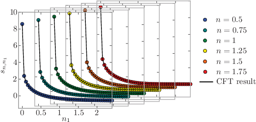
Refer to caption
Figure 2: Numerical measures (dots) of Affleck-Ludwig boundary entropy for dense loops, as functions of nn and n1n_{1}. Solid lines are given by (13).

3 The trousers trick

In the remainder of this paper we will always consider systems with boundaries, and boundary CFTs. As explained in section 1, we need to identify a lattice version of the conformal state L−2|0⟩L_{-2}\left|0\right>. To do this, we first note that L−2L_{-2} generates a conformal transformation that maps the half-plane with an infinitesimal vertical slit onto the half-plane itself. This very basic idea is at the heart of the relation between the operator formalism of CFT and the celebrated Schramm-Loewner Evolution [41, 42]. By turning this infinitesimal conformal transformation into a finite one, we will be able to build its lattice version.

We proceed as in [41, 42]: consider the sequence of infinitesimal transformations z↦z+d​g​(z)z\mapsto z+{\rm d}g(z) where d​g​(z)=d​t/(2​z){\rm d}g(z)={\rm d}t/(2z). This is the infinitesimal version of the transformation

gt​(z)=z2+tg_{t}(z)=\sqrt{z^{2}+t} (14)

in the sense that ∂∂t​gt​(z)=1/(2​gt​(z))\frac{\partial}{\partial t}g_{t}(z)=1/(2g_{t}(z)). The tranformation (14) maps conformally the half-plane minus a slit of height t\sqrt{t} onto the half-plane (figure 3). Taking z=gt−1​(w)z=g^{-1}_{t}(w), where ww is now a point in the upper half-plane, we have

(∂gt∂t)∘gt−1​(w)=1/2w\left(\frac{\partial g_{t}}{\partial t}\right)\circ g_{t}^{-1}(w)=\frac{1/2}{w} (15)

so if FF is an arbitrary function defined on the half-plane, it gets changed under the infinitesimal transformation d​g{\rm d}g by

d​F=d​t/2w​(∂wF)=−d​t2​l−2​F{\rm d}F=\frac{{\rm d}t/2}{w}\left(\partial_{w}F\right)=-\frac{{\rm d}t}{2}\;l_{-2}F (16)

where l−k=−w−k+1∂wl_{-k}=-w^{-k+1}\partial_{w} is a generator of the Witt algebra. If G~g:F↦F∘g\tilde{G}_{g}:F\mapsto F\circ g, we see that equations (15) and (16) can be written G~gt−1∘∂G~gt∂t=−(1/2)​l−2\tilde{G}^{-1}_{g_{t}}\circ\frac{\partial\tilde{G}_{g_{t}}}{\partial t}=-(1/2)l_{-2} (the order comes from G~f∘h=G~h∘G~f\tilde{G}_{f\circ h}=\tilde{G}_{h}\circ\tilde{G}_{f}). We have thus obtained a differential equation which allows to compute G~gt\tilde{G}_{g_{t}}. This operator maps a function FF (defined on the upper half-plane) onto a function F∘gtF\circ g_{t} (defined in the upper half-plane minus a slit as in Fig. 3). In CFT, we want to act on the Verma modules rather than on simple functions. Thus we are looking for a linear operator GgtG_{g_{t}} that maps a state |s⟩\left|s\right> of the theory in the upper half-plane geometry onto Ggt|s⟩G_{g_{t}}\left|s\right>, encoding the new geometry. Turning the Witt generators into the Virasoro ones, we get

Ggt−1.∂Ggt∂t=−12​L−2G^{-1}_{g_{t}}.\frac{\partial G_{g_{t}}}{\partial t}=-\frac{1}{2}L_{-2} (17)

and of course at t=0t=0 the operator is the identity Gg0=1G_{g_{0}}=1, so we end up with

Ggt=exp⁡(−t2​L−2).G_{g_{t}}=\exp\left(-\frac{t}{2}L_{-2}\right). (18)
|Trous.⟩\left|\rm{Trous.}\right>L/2L/2L/2L/2∼\sim|Trous.⟩\left|\rm{Trous.}\right>g1g_{1}|0⟩\left|0\right>
Figure 3: The trousers geometry can be developed on the half-plane by the function g1​(z)=z2+1g_{1}(z)=\sqrt{z^{2}+1}. This operation is encoded in the state |Trousers⟩=e−12​L−2|0⟩\left|\rm{Trousers}\right>={\rm e}^{-\frac{1}{2}L_{-2}}\left|0\right>.

The fact that the action of L−2L_{-2} encodes a small slit in the original geometry motivates the introduction of the “trousers” geometry (Fig. 3). Indeed, it is well-known that a CFT on the infinite strip of width LL is equivalent to a CFT in the upper half-plane (the latter can be mapped on the former by the transformation z→w⁡(z)=Lπ​log⁡zz\to w(z)=\frac{L}{\pi}\log z). Cutting a small slit in the half-plane is then equivalent to cutting a slit in the infinite strip, dividing it into two strips of width L/2L/2 up to some height. This is the trousers geometry (Fig. 3). The ground state of the translation operator along the strip πL​(L0−c24)\frac{\pi}{L}\left(L_{0}-\frac{c}{24}\right) is |0⟩\left|0\right>. It is different from the ground state of the system with two legs of width L/2L/2, which is a tensor product |Trousers⟩≡|0⟩′⊗|0⟩′\left|\rm{Trousers}\right>\equiv\left|0\right>^{\prime}\otimes\left|0\right>^{\prime} if |0⟩′\left|0\right>^{\prime} is the ground state of width L/2L/2. Formula (18) shows that

|Trousers⟩=e−12​L−2|0⟩=|0⟩−12L−2|0⟩+…\left|\rm{Trousers}\right>\;=\;e^{-\frac{1}{2}L_{-2}}\left|0\right>\;=\;\left|0\right>-\frac{1}{2}L_{-2}\left|0\right>+\dots (19)

We get a lattice version of the trousers geometry if we glue together two ground states of the transfer matrix TL/2T_{L/2} or Hamiltonian HL/2H_{L/2}, i.e., |Trousers⟩L≡|0⟩L/2⊗|0⟩L/2\left|\rm{Trousers}\right>_{L}\equiv\left|0\right>_{L/2}\otimes\left|0\right>_{L/2} (see Fig. 4 for example).

4 Measure of bb

While we are mostly interested in polymers and percolation in this paper, there remains a certain variety of models one can consider. Indeed, one of the difficulties of the field is that geometrical problems are not defined in the usual terms of local degrees of freedom and hamiltonians, and the purported LCFT one is after might well depend on the kind of questions one wants to ask. For percolation for instance, one can decide to focus on the boundaries of clusters, or on the six-vertex model version, or on one of the supersymmetric versions [43, 24, 18]. We will discuss this point more in the conclusion. For now, we start with the six-vertex model (or equivalently the XXZ spin chain), largely for pedagogical reasons. We then move on to a purely geometrical set-up for the case of polymers.

4.1 Measure of bb in the XXZ spin chain at q=ei​π3q={\rm e}^{i\frac{\pi}{3}}

We consider the Uq​(s​l2)U_{q}(sl_{2}) symmetric XXZ spin chain with q=ei​π3q={\rm e}^{i\frac{\pi}{3}} [39]. The Hamiltonian with open boundary conditions is

HL=∑i=1L−1[σix​σi+1x+σiy​σi+1y+q+q−12​σiz​σi+1z]+q−q−12​(σ1z−σLz).H_{L}=\sum_{i=1}^{L-1}\left[\sigma^{x}_{i}\sigma_{i+1}^{x}+\sigma^{y}_{i}\sigma_{i+1}^{y}+\frac{q+q^{-1}}{2}\sigma^{z}_{i}\sigma_{i+1}^{z}\right]+\frac{q-q^{-1}}{2}\left(\sigma_{1}^{z}-\sigma_{L}^{z}\right)\;. (20)

Although HLH_{L} is not hermitian, its spectrum is real. When q=ei​π3q={\rm e}^{i\frac{\pi}{3}} it has a Jordan cell structure [39] for L≥4L\geq 4.

The low-energy spectrum of HLH_{L} is described by a CFT with c=0c=0. HLH_{L} and the Virasoro generator are related by HL≈E0+π​vFL​L0+𝒪⁡(1L2)H_{L}\approx E_{0}+\frac{\pi v_{F}}{L}L_{0}+\mathcal{O}\left(\frac{1}{L^{2}}\right) when L→∞L\rightarrow\infty. Here the Fermi velocity is vF=3​3v_{F}=3\sqrt{3} [39].

Scalar product for the XXZ chain.

What is the right scalar product for the XXZ chain? We claim that this is just the Euclidean scalar product in the spin basis, treating qq as a formal parameter (i.e., without complex conjugation). For example, the qq-singlet state |s⟩2≡q−1/2↑↓−q1/2↓↑\left|s\right>_{2}\equiv q^{-1/2}\uparrow\downarrow-q^{1/2}\downarrow\uparrow has a norm squared ⟨s|s⟩22=q+q−1{\vphantom{\left<s|s\right>}}{}_{2}\left<s|s\right>_{2}=q+q^{-1} (if qq had been conjugated, one would have found ⟨s|s⟩22=|q|+|q|−1=2{\vphantom{\left<s|s\right>}}{}_{2}\left<s|s\right>_{2}=|q|+|q|^{-1}=2).

There are different ways of seeing that this is the right scalar product. One simple way is that the XXZ chain can be mapped on the dense loop model introduced in section 22, with a weight n=q+q−1n=q+q^{-1} for each closed loop. This mapping consists in replacing each qq-singlet by a half-loop …⊗(q−1/2↑↓−q1/2↓↑)⊗…→…      …\;\ldots\otimes\left(q^{-1/2}\uparrow\downarrow-q^{1/2}\downarrow\uparrow\right)\otimes\dots\;\rightarrow\;\dots\hbox to6.49pt{\vbox to7.91pt{\pgfpicture\makeatletter\hbox{\hskip 0.4pt\lower-7.51318pt\hbox to0.0pt{\lxSVG@begingroup@{_scopebegin=1} \lxSVG@begingroup@{stroke=#000000} \lxSVG@begingroup@{fill=#000000} \lxSVG@setlinewidth{\the\pgflinewidth}\lxSVG@begingroup@{stroke-width=0.4pt} \lx@inpgf@ignorespaces\nullfont\hbox to0.0pt{\lxSVG@begingroup@{_scopebegin=1} {}{{}}{}{{}{}{\lx@inpgf@ignorespaces}{{\lx@inpgf@ignorespaces}}{{{{}{}{}{}}} {{}{}{}{}}}}{} {} {} {} {}{}\lxSVG@begingroup@{_scopebegin=1} \lxSVG@setlinewidth{\the\pgflinewidth}\lxSVG@begingroup@{stroke-width=0.8pt} \lx@inpgf@ignorespaces{}\lxSVG@stroke\lxSVG@drawpath@unclipped{M 0 0 C 0 -5.44 1.76 -9.84 3.94 -9.84 C 6.11 -9.84 7.87 -5.44 7.87 0}{fill:none} \lx@inpgf@ignorespaces \lxSVG@closescope \lxSVG@closescope {\lx@inpgf@ignorespaces}{\lx@inpgf@ignorespaces}{\lx@inpgf@ignorespaces}\hss}\lxSVG@discardpath\lxSVG@closescope \hss}}\lxSVG@closescope\endpgfpicture}}\dots\;. Thus the loop scalar product, as defined in section 2.22.2, is the same as the one we are considering now. In particular, this scalar product can be negative, and we have already seen that this is what makes it a good candidate for being a finite-size version of the Virasoro scalar product in the scaling limit. Another check that this scalar product is the right one is that HLH_{L} becomes hermitian for this new scalar product. This is a property that should be expected, because HLH_{L} is related to L0L_{0} in the scaling limit, and L0L_{0} is hermitian for the Virasoro scalar product.

A detailed example: L=4L=4.

To explain our strategy, let us discuss in full detail the case of the lowest interesting even size. We consider the Sz=0S^{z}=0 sector only (note that in general [HL,Sz]=0\left[H_{L},S^{z}\right]=0). In the basis {↑↑↓↓,↑↓↑↓,↑↓↓↑,↓↑↑↓,↓↑↓↑,↓↓↑↑}\left\{\uparrow\uparrow\downarrow\downarrow,\uparrow\downarrow\uparrow\downarrow,\uparrow\downarrow\downarrow\uparrow,\downarrow\uparrow\uparrow\downarrow,\downarrow\uparrow\downarrow\uparrow,\downarrow\downarrow\uparrow\uparrow\right\}, the Hamiltonian is

H4=(12+i​3202−32+i​32202−120220−122022−32−i​320212−i​3)H_{4}=\left(\begin{array}[]{cccccc}\frac{1}{2}+i\sqrt{3}&2&0&&&\\ \\ 2&-\frac{3}{2}+i\sqrt{3}&2&2\\ \\ 0&2&-\frac{1}{2}&0&2\\ \\ &2&0&-\frac{1}{2}&2&0\\ \\ &&2&2&-\frac{3}{2}-i\sqrt{3}&2\\ \\ &&&0&2&\frac{1}{2}-i\sqrt{3}\end{array}\right)

and it can be put in Jordan form in a suitable basis {|0⟩4,|1⟩4,|2⟩4,|3⟩4,|3~′⟩4,|4⟩4}\left\{\left|0\right>_{4},\left|1\right>_{4},\left|2\right>_{4},\left|3\right>_{4},\left|\tilde{3}^{\prime}\right>_{4},\left|4\right>_{4}\right\}

H4=(−9/2−2​2−12−123210322​2−12)H_{4}=\left(\begin{array}[]{cccccc}-9/2&\\ \\ &-2\sqrt{2}-\frac{1}{2}\\ \\ &&-\frac{1}{2}&\\ \\ &&&\frac{3}{2}&1\\ \\ &&&0&\frac{3}{2}\\ \\ &&&&&2\sqrt{2}-\frac{1}{2}\end{array}\right)

We give the states |0⟩4\left|0\right>_{4}, |3⟩4\left|3\right>_{4} and |3~′⟩4\left|\tilde{3}^{\prime}\right>_{4} only (the other ones are not important in what follows)

|0⟩4=16(−1+i3)↑↑↓↓+13(2−i3)↑↓↑↓−23(↑↓↓↑+↓↑↑↓)+13​(2+i​3)↓↑↓↑−16​(1+i​3)↓↓↑↑|3⟩4=12(1+i3)↑↑↓↓+12(−1−i3)↑↓↑↓−(↑↓↓↑+↓↑↑↓)+12​(−1+i​3)↓↑↓↑+12​(1−i​3)↓↓↑↑|3~′⟩4=14(1−i3)↑↑↓↓−18(1+i33)(↑↓↓↑+↓↑↑↓)+18​(−7−i​3)↓↑↓↑+38​(−3+i​3)↓↓↑↑\begin{array}[]{rcl}\left|0\right>_{4}&=&\frac{1}{6}\left(-1+i\sqrt{3}\right)\uparrow\uparrow\downarrow\downarrow+\frac{1}{3}\left(2-i\sqrt{3}\right)\uparrow\downarrow\uparrow\downarrow-\frac{2}{3}\left(\uparrow\downarrow\downarrow\uparrow+\downarrow\uparrow\uparrow\downarrow\right)\\ &&+\frac{1}{3}\left(2+i\sqrt{3}\right)\downarrow\uparrow\downarrow\uparrow-\frac{1}{6}\left(1+i\sqrt{3}\right)\downarrow\downarrow\uparrow\uparrow\\ \left|3\right>_{4}&=&\frac{1}{2}\left(1+i\sqrt{3}\right)\uparrow\uparrow\downarrow\downarrow+\frac{1}{2}\left(-1-i\sqrt{3}\right)\uparrow\downarrow\uparrow\downarrow-\left(\uparrow\downarrow\downarrow\uparrow+\downarrow\uparrow\uparrow\downarrow\right)\\ &&+\frac{1}{2}\left(-1+i\sqrt{3}\right)\downarrow\uparrow\downarrow\uparrow+\frac{1}{2}\left(1-i\sqrt{3}\right)\downarrow\downarrow\uparrow\uparrow\\ \left|\tilde{3}^{\prime}\right>_{4}&=&\frac{1}{4}\left(1-i\sqrt{3}\right)\uparrow\uparrow\downarrow\downarrow-\frac{1}{8}\left(1+i3\sqrt{3}\right)\left(\uparrow\downarrow\downarrow\uparrow+\downarrow\uparrow\uparrow\downarrow\right)\\ &&+\frac{1}{8}\left(-7-i\sqrt{3}\right)\downarrow\uparrow\downarrow\uparrow+\frac{3}{8}\left(-3+i\sqrt{3}\right)\downarrow\downarrow\uparrow\uparrow\\ \end{array}

With the above scalar product (i.e., without complex conjugation), we see that

4⟨0|0⟩4=14⟨3|3⟩4=04⟨3|3~′⟩4=−34.\begin{array}[]{rcl}{\vphantom{\left<0|0\right>}}{}_{4}\left<0|0\right>_{4}&=&1\\ {\vphantom{\left<3|3\right>}}{}_{4}\left<3|3\right>_{4}&=&0\\ {\vphantom{\left<3|\tilde{3}^{\prime}\right>}}{}_{4}\left<3|\tilde{3}^{\prime}\right>_{4}&=&-\frac{3}{4}.\end{array}

Note that |3~′⟩4\left|\tilde{3}^{\prime}\right>_{4} is only defined up to some additional term |3~′⟩4+λ|3⟩4\left|\tilde{3}^{\prime}\right>_{4}+\lambda\left|3\right>_{4}. The scalar product ⟨3~′|3~′⟩44{\vphantom{\left<\tilde{3}^{\prime}|\tilde{3}^{\prime}\right>}}{}_{4}\left<\tilde{3}^{\prime}|\tilde{3}^{\prime}\right>_{4} is not invariant under such a transformation, so this is certainly not a well-defined quantity. On the contrary, ⟨3|3~′⟩44{\vphantom{\left<3|\tilde{3}^{\prime}\right>}}{}_{4}\left<3|\tilde{3}^{\prime}\right>_{4} seems well-defined. However, since ⟨3|3⟩44=0{\vphantom{\left<3|3\right>}}{}_{4}\left<3|3\right>_{4}=0, we see that there is still some undetermination: the structure of the Jordan cell is the same if one rescales |3⟩4→α|3⟩4\left|3\right>_{4}\rightarrow\alpha\left|3\right>_{4} and |3~′⟩4→α|3~′⟩4\left|\tilde{3}^{\prime}\right>_{4}\rightarrow\alpha\left|\tilde{3}^{\prime}\right>_{4}, thus changing the scalar product ⟨3|3~′⟩44{\vphantom{\left<3|\tilde{3}^{\prime}\right>}}{}_{4}\left<3|\tilde{3}^{\prime}\right>_{4}. The whole point of the trousers trick will be to get rid of this undetermined factor α\alpha.

To prepare the comparison with CFT, we introduce another normalization. Let |3~⟩4≡π​vF4|3~′⟩4\left|\tilde{3}\right>_{4}\equiv\frac{\pi v_{F}}{4}\left|\tilde{3}^{\prime}\right>_{4}, then in the basis {|0⟩4,|3⟩4,|3~⟩4}\left\{\left|0\right>_{4},\left|3\right>_{4},\left|\tilde{3}\right>_{4}\right\} we have

4π​vF​(H4−E4,0)=(0Δ41Δ4)\frac{4}{\pi v_{F}}\left(H_{4}-E_{4,0}\right)=\left(\begin{array}[]{ccc}0\\ &\Delta_{4}&1\\ &&\Delta_{4}\end{array}\right)

where E4,0=−92E_{4,0}=-\frac{9}{2} is the ground state energy, and Δ4=4π​vF​(32−E4,0)=4​3π\Delta_{4}=\frac{4}{\pi v_{F}}\left(\frac{3}{2}-E_{4,0}\right)=\frac{4\sqrt{3}}{\pi}. The operator Lπ​vF​(HL−EL,0)\frac{L}{\pi v_{F}}\left(H_{L}-E_{L,0}\right) should be viewed as a lattice version of L0L_{0}, as follows from the boundary analog of (11).

We still have to build the state |Trousers⟩4\left|\rm{Trousers}\right>_{4} for L=4L=4. This is just a tensor product of two times the ground state of H2H_{2}, which is a Uq​(s​l2)U_{q}(sl_{2}) singlet: |s⟩2≡q−1/2↑↓−q1/2↓↑\left|s\right>_{2}\equiv q^{-1/2}\uparrow\downarrow-q^{1/2}\downarrow\uparrow.

|Trousers⟩4≡|s⟩2⊗|s⟩2=(12−i32)↑↓↑↓−(↑↓↓↑+↓↑↑↓)+(12+i32)↓↑↓↑.\left|\rm{Trousers}\right>_{4}\;\equiv\;\left|s\right>_{2}\otimes\left|s\right>_{2}\;=\;\left(\frac{1}{2}-i\frac{\sqrt{3}}{2}\right)\uparrow\downarrow\uparrow\downarrow-\left(\uparrow\downarrow\downarrow\uparrow+\downarrow\uparrow\uparrow\downarrow\right)+\left(\frac{1}{2}+i\frac{\sqrt{3}}{2}\right)\downarrow\uparrow\downarrow\uparrow.

Note that it is normalized such that ⟨Trousers|0⟩44=1{\vphantom{\left<\rm{Trousers}|0\right>}}{}_{4}\left<\rm{Trousers}|0\right>_{4}=1, in order to match ⟨0|0⟩=1\langle 0|0\rangle=1 when using (19).

Now we are ready to define a lattice quantity b⁡(L=4)b(L=4), that is invariant under a global rescaling of the Jordan cell |3⟩4→α|3⟩4\left|3\right>_{4}\rightarrow\alpha\left|3\right>_{4} and |3~⟩4→|3~⟩4\left|\tilde{3}\right>_{4}\rightarrow\left|\tilde{3}\right>_{4} and that will later correspond to bb in the L→∞L\rightarrow\infty limit (see below):

b⁡(4)≡ 4​(4⟨Trousers|3~⟩4)24⟨3|3~⟩4.b(4)\;\equiv\;4\;\frac{\left({\vphantom{\left<\rm{Trousers}|\tilde{3}\right>}}{}_{4}\left<\rm{Trousers}|\tilde{3}\right>_{4}\right)^{2}}{{\vphantom{\left<3|\tilde{3}\right>}}{}_{4}\left<3|\tilde{3}\right>_{4}}.

With the above expressions of the states one gets b⁡(4)=−3​π4=−1.3603495​…b(4)=-\frac{\sqrt{3}\pi}{4}=-1.3603495\dots\;.

General strategy.

We have to restrict to sizes LL that are multiples of 44, because one needs to build the state |Trousers⟩\left|\rm{Trousers}\right> out of the ground state of HL/2H_{L/2} in the Sz=0S^{z}=0 sector, so L/2L/2 must be even.

If the spectrum of HLH_{L} in the Sz=0S^{z}=0 sector is EL,0<EL,1<EL,2<…E_{L,0}<E_{L,1}<E_{L,2}<\dots then EL,3E_{L,3} is always twice degenerate (for L≥4L\geq 4). Let {|3⟩L,|3~⟩L}\left\{\left|3\right>_{L},\left|\tilde{3}\right>_{L}\right\} be a basis of this equal-energy subspace, so that the lattice version of L0L_{0} reads

Lπ​vF​(HL−EL,0)=(ΔL10ΔL),\frac{L}{\pi v_{F}}\left(H_{L}-E_{L,0}\right)=\left(\begin{array}[]{cc}\Delta_{L}&1\\ 0&\Delta_{L}\end{array}\right)\,, (21)

where ΔL≡Lπ​vF​(EL,3−EL,0)→2\Delta_{L}\equiv\frac{L}{\pi v_{F}}\left(E_{L,3}-E_{L,0}\right)\to 2 as L→∞L\to\infty.

Again, there is an undetermined overall normalization because ⟨3|3⟩LL=0{\vphantom{\left<3|3\right>}}{}_{L}\left<3|3\right>_{L}=0 (with the same scalar product as above). The trousers trick is used again to define a normalization-independent lattice quantity b⁡(L)b(L) as in the case L=4L=4. We normalize |0⟩L\left|0\right>_{L} and |Trousers⟩L\left|\rm{Trousers}\right>_{L} such that ⟨Trousers|0⟩LL=L⟨0|0⟩L= 1{\vphantom{\left<\rm{Trousers}|0\right>}}{}_{L}\left<\rm{Trousers}|0\right>_{L}\;=\;{\vphantom{\left<0|0\right>}}_{L}\left<0|0\right>_{L}\;=\;1. Then define

b⁡(L)≡4​(L⟨Trousers|3~⟩L)2L⟨3|3~⟩L.b(L)\equiv 4\frac{\left({\vphantom{\left<\rm{Trousers}|\tilde{3}\right>}}{}_{L}\left<\rm{Trousers}|\tilde{3}\right>_{L}\right)^{2}}{{\vphantom{\left<3|\tilde{3}\right>}}{}_{L}\left<3|\tilde{3}\right>_{L}}. (22)

When L→∞L\to\infty, we expect |3⟩L∼αL−2|0⟩\left|3\right>_{L}\sim\alpha L_{-2}\left|0\right> and |3~⟩L∼αΦ1,5|0⟩\left|\tilde{3}\right>_{L}\sim\alpha\Phi_{1,5}\left|0\right>. Using relation (19) we get

b⁡(L)⟶L→∞4​(α⁡⟨Trousers|Φ1,5|0⟩)2α2​⟨0|L2​Φ1,5|0⟩=⟨0|L2​Φ1,5|0⟩=⟨T|t⟩=b.b(L)\quad\underset{L\rightarrow\infty}{\longrightarrow}\quad 4\;\frac{\left(\alpha\left<\rm{Trousers}|\Phi_{1,5}|0\right>\right)^{2}}{\alpha^{2}\left<0|L_{2}\Phi_{1,5}|0\right>}\;=\;\left<0|L_{2}\Phi_{1,5}|0\right>\;=\;\langle T|t\rangle\;=\;b. (23)

Numerical results are given below (Tab. 1).

4.2 Measure of bb in the dilute polymers model

We consider a dilute polymers model on the honeycomb lattice. It is defined by the tranfer matrix (in the picture L=6L=6)

TL=T_{L}\;=

where each losange is a sum over eight configurations with weight xx per monomer:

11xxxxx2x^{2}x2x^{2}x2x^{2}x2x^{2}x2x^{2}

The boundary triangles can appear with or without monomers, with weights xx or 11. There are no closed loops in this model (i.e., the loop weight is n=0n=0). This model is the n→0n\rightarrow 0 limit of the O⁡(n)O(n) model. Its critical point [35] is x=(2+2)−1/2x=(2+\sqrt{2})^{-1/2}, and it corresponds in the scaling limit to dilute polymers (or self-avoiding walks).

The transfer matrix TLT_{L} acts on configuration states that contain half-loops and empty sites (marked with dots), such as |                    ⟩\left|\;\hbox to29.54pt{\vbox to8.2pt{\pgfpicture\makeatletter\hbox{\hskip 0.68436pt\lower-7.51318pt\hbox to0.0pt{\lxSVG@begingroup@{_scopebegin=1} \lxSVG@begingroup@{stroke=#000000} \lxSVG@begingroup@{fill=#000000} \lxSVG@setlinewidth{\the\pgflinewidth}\lxSVG@begingroup@{stroke-width=0.4pt} \lx@inpgf@ignorespaces\nullfont\hbox to0.0pt{\lxSVG@begingroup@{_scopebegin=1} {}{{}}{}{{}{}{\lx@inpgf@ignorespaces}{{\lx@inpgf@ignorespaces}}{{{{}{}{}{}}} {{}{}{}{}}}}{} {} {} {} {}{}\lxSVG@begingroup@{_scopebegin=1} \lxSVG@setlinewidth{\the\pgflinewidth}\lxSVG@begingroup@{stroke-width=0.8pt} \lx@inpgf@ignorespaces{}\lxSVG@stroke\lxSVG@drawpath@unclipped{M 15.75 0 C 15.75 -5.44 21.04 -9.84 27.56 -9.84 C 34.08 -9.84 39.37 -5.44 39.37 0}{fill:none} \lx@inpgf@ignorespaces \lxSVG@closescope {}{{}}{}{{{}}{\lx@inpgf@ignorespaces}{}{}{}{}{}{}{}}\lxSVG@begingroup@{_scopebegin=1} \lxSVG@setlinewidth{\the\pgflinewidth}\lxSVG@begingroup@{stroke-width=0.8pt} \lx@inpgf@ignorespaces{}\lxSVG@stroke\lxSVG@drawpath@unclipped{M 0 0 M 0.39 0 C 0.39 0.22 0.22 0.39 0 0.39 C -0.22 0.39 -0.39 0.22 -0.39 0 C -0.39 -0.22 -0.22 -0.39 0 -0.39 C 0.22 -0.39 0.39 -0.22 0.39 0 Z M 0 0}{fill:none} \lx@inpgf@ignorespaces \lxSVG@closescope {}{{}}{}{{{}}{\lx@inpgf@ignorespaces}{}{}{}{}{}{}{}}\lxSVG@begingroup@{_scopebegin=1} \lxSVG@setlinewidth{\the\pgflinewidth}\lxSVG@begingroup@{stroke-width=0.8pt} \lx@inpgf@ignorespaces{}\lxSVG@stroke\lxSVG@drawpath@unclipped{M 7.87 0 M 8.27 0 C 8.27 0.22 8.09 0.39 7.87 0.39 C 7.66 0.39 7.48 0.22 7.48 0 C 7.48 -0.22 7.66 -0.39 7.87 -0.39 C 8.09 -0.39 8.27 -0.22 8.27 0 Z M 7.87 0}{fill:none} \lx@inpgf@ignorespaces \lxSVG@closescope {}{{}}{}{{{}}{\lx@inpgf@ignorespaces}{}{}{}{}{}{}{}}\lxSVG@begingroup@{_scopebegin=1} \lxSVG@setlinewidth{\the\pgflinewidth}\lxSVG@begingroup@{stroke-width=0.8pt} \lx@inpgf@ignorespaces{}\lxSVG@stroke\lxSVG@drawpath@unclipped{M 23.62 0 M 24.02 0 C 24.02 0.22 23.84 0.39 23.62 0.39 C 23.4 0.39 23.23 0.22 23.23 0 C 23.23 -0.22 23.4 -0.39 23.62 -0.39 C 23.84 -0.39 24.02 -0.22 24.02 0 Z M 23.62 0}{fill:none} \lx@inpgf@ignorespaces \lxSVG@closescope {}{{}}{}{{{}}{\lx@inpgf@ignorespaces}{}{}{}{}{}{}{}}\lxSVG@begingroup@{_scopebegin=1} \lxSVG@setlinewidth{\the\pgflinewidth}\lxSVG@begingroup@{stroke-width=0.8pt} \lx@inpgf@ignorespaces{}\lxSVG@stroke\lxSVG@drawpath@unclipped{M 31.5 0 M 31.89 0 C 31.89 0.22 31.71 0.39 31.5 0.39 C 31.28 0.39 31.1 0.22 31.1 0 C 31.1 -0.22 31.28 -0.39 31.5 -0.39 C 31.71 -0.39 31.89 -0.22 31.89 0 Z M 31.5 0}{fill:none} \lx@inpgf@ignorespaces \lxSVG@closescope \lxSVG@closescope {\lx@inpgf@ignorespaces}{\lx@inpgf@ignorespaces}{\lx@inpgf@ignorespaces}\hss}\lxSVG@discardpath\lxSVG@closescope \hss}}\lxSVG@closescope\endpgfpicture}}\;\right> or |                 ⟩\left|\;\hbox to29.54pt{\vbox to8.2pt{\pgfpicture\makeatletter\hbox{\hskip 0.4pt\lower-7.51318pt\hbox to0.0pt{\lxSVG@begingroup@{_scopebegin=1} \lxSVG@begingroup@{stroke=#000000} \lxSVG@begingroup@{fill=#000000} \lxSVG@setlinewidth{\the\pgflinewidth}\lxSVG@begingroup@{stroke-width=0.4pt} \lx@inpgf@ignorespaces\nullfont\hbox to0.0pt{\lxSVG@begingroup@{_scopebegin=1} {}{{}}{}{{}{}{\lx@inpgf@ignorespaces}{{\lx@inpgf@ignorespaces}}{{{{}{}{}{}}} {{}{}{}{}}}}{} {} {} {} {}{}\lxSVG@begingroup@{_scopebegin=1} \lxSVG@setlinewidth{\the\pgflinewidth}\lxSVG@begingroup@{stroke-width=0.8pt} \lx@inpgf@ignorespaces{}\lxSVG@stroke\lxSVG@drawpath@unclipped{M 0 0 C 0 -5.44 7.05 -9.84 15.75 -9.84 C 24.45 -9.84 31.5 -5.44 31.5 0}{fill:none} \lx@inpgf@ignorespaces \lxSVG@closescope {}{{}}{}{{}{}{\lx@inpgf@ignorespaces}{{\lx@inpgf@ignorespaces}}{{{{}{}{}{}}} {{}{}{}{}}}}{} {} {} {} {}{}\lxSVG@begingroup@{_scopebegin=1} \lxSVG@setlinewidth{\the\pgflinewidth}\lxSVG@begingroup@{stroke-width=0.8pt} \lx@inpgf@ignorespaces{}\lxSVG@stroke\lxSVG@drawpath@unclipped{M 15.75 0 C 15.75 -3.26 17.51 -5.91 19.69 -5.91 C 21.86 -5.91 23.62 -3.26 23.62 0}{fill:none} \lx@inpgf@ignorespaces \lxSVG@closescope {}{{}}{}{{{}}{\lx@inpgf@ignorespaces}{}{}{}{}{}{}{}}\lxSVG@begingroup@{_scopebegin=1} \lxSVG@setlinewidth{\the\pgflinewidth}\lxSVG@begingroup@{stroke-width=0.8pt} \lx@inpgf@ignorespaces{}\lxSVG@stroke\lxSVG@drawpath@unclipped{M 7.87 0 M 8.27 0 C 8.27 0.22 8.09 0.39 7.87 0.39 C 7.66 0.39 7.48 0.22 7.48 0 C 7.48 -0.22 7.66 -0.39 7.87 -0.39 C 8.09 -0.39 8.27 -0.22 8.27 0 Z M 7.87 0}{fill:none} \lx@inpgf@ignorespaces \lxSVG@closescope {}{{}}{}{{{}}{\lx@inpgf@ignorespaces}{}{}{}{}{}{}{}}\lxSVG@begingroup@{_scopebegin=1} \lxSVG@setlinewidth{\the\pgflinewidth}\lxSVG@begingroup@{stroke-width=0.8pt} \lx@inpgf@ignorespaces{}\lxSVG@stroke\lxSVG@drawpath@unclipped{M 39.37 0 M 39.76 0 C 39.76 0.22 39.59 0.39 39.37 0.39 C 39.15 0.39 38.98 0.22 38.98 0 C 38.98 -0.22 39.15 -0.39 39.37 -0.39 C 39.59 -0.39 39.76 -0.22 39.76 0 Z M 39.37 0}{fill:none} \lx@inpgf@ignorespaces \lxSVG@closescope \lxSVG@closescope {\lx@inpgf@ignorespaces}{\lx@inpgf@ignorespaces}{\lx@inpgf@ignorespaces}\hss}\lxSVG@discardpath\lxSVG@closescope \hss}}\lxSVG@closescope\endpgfpicture}}\;\right> for L=6L=6. We also have to encode the fact that polymers are already in the system when one applies TLT_{L} the first time, or in other words that they are “connected to the infinite past”. We thus introduce strings (unpaired points interpreted as loop segments connecting to the infinite past) like for example |                    ⟩\left|\;\hbox to29.25pt{\vbox to8.2pt{\pgfpicture\makeatletter\hbox{\hskip 0.4pt\lower-7.51318pt\hbox to0.0pt{\lxSVG@begingroup@{_scopebegin=1} \lxSVG@begingroup@{stroke=#000000} \lxSVG@begingroup@{fill=#000000} \lxSVG@setlinewidth{\the\pgflinewidth}\lxSVG@begingroup@{stroke-width=0.4pt} \lx@inpgf@ignorespaces\nullfont\hbox to0.0pt{\lxSVG@begingroup@{_scopebegin=1} {}{{}}{}{{}{}{\lx@inpgf@ignorespaces}{{\lx@inpgf@ignorespaces}}{{{{}{}{}{}}} {{}{}{}{}}}}{} {} {} {} {}{}\lxSVG@begingroup@{_scopebegin=1} \lxSVG@setlinewidth{\the\pgflinewidth}\lxSVG@begingroup@{stroke-width=0.8pt} \lx@inpgf@ignorespaces{}\lxSVG@stroke\lxSVG@drawpath@unclipped{M 0 0 C 0 -5.44 1.76 -9.84 3.94 -9.84 C 6.11 -9.84 7.87 -5.44 7.87 0}{fill:none} \lx@inpgf@ignorespaces \lxSVG@closescope {}{{}}{}{{{}}{\lx@inpgf@ignorespaces}{}{}{}{}{}{}{}}\lxSVG@begingroup@{_scopebegin=1} \lxSVG@setlinewidth{\the\pgflinewidth}\lxSVG@begingroup@{stroke-width=0.8pt} \lx@inpgf@ignorespaces{}\lxSVG@stroke\lxSVG@drawpath@unclipped{M 15.75 0 M 16.14 0 C 16.14 0.22 15.97 0.39 15.75 0.39 C 15.53 0.39 15.35 0.22 15.35 0 C 15.35 -0.22 15.53 -0.39 15.75 -0.39 C 15.97 -0.39 16.14 -0.22 16.14 0 Z M 15.75 0}{fill:none} \lx@inpgf@ignorespaces \lxSVG@closescope {}{{}}{}{{{}}{\lx@inpgf@ignorespaces}{}{}{}{}{}{}{}}\lxSVG@begingroup@{_scopebegin=1} \lxSVG@setlinewidth{\the\pgflinewidth}\lxSVG@begingroup@{stroke-width=0.8pt} \lx@inpgf@ignorespaces{}\lxSVG@stroke\lxSVG@drawpath@unclipped{M 31.5 0 M 31.89 0 C 31.89 0.22 31.71 0.39 31.5 0.39 C 31.28 0.39 31.1 0.22 31.1 0 C 31.1 -0.22 31.28 -0.39 31.5 -0.39 C 31.71 -0.39 31.89 -0.22 31.89 0 Z M 31.5 0}{fill:none} \lx@inpgf@ignorespaces \lxSVG@closescope {}{{}}{} {{}{}}{}\lxSVG@begingroup@{_scopebegin=1} \lxSVG@setlinewidth{\the\pgflinewidth}\lxSVG@begingroup@{stroke-width=0.8pt} \lx@inpgf@ignorespaces{}\lxSVG@stroke\lxSVG@drawpath@unclipped{M 23.62 -9.84 L 23.62 0}{fill:none} \lx@inpgf@ignorespaces \lxSVG@closescope {}{{}}{} {{}{}}{}\lxSVG@begingroup@{_scopebegin=1} \lxSVG@setlinewidth{\the\pgflinewidth}\lxSVG@begingroup@{stroke-width=0.8pt} \lx@inpgf@ignorespaces{}\lxSVG@stroke\lxSVG@drawpath@unclipped{M 39.37 -9.84 L 39.37 0}{fill:none} \lx@inpgf@ignorespaces \lxSVG@closescope \lxSVG@closescope {\lx@inpgf@ignorespaces}{\lx@inpgf@ignorespaces}{\lx@inpgf@ignorespaces}\hss}\lxSVG@discardpath\lxSVG@closescope \hss}}\lxSVG@closescope\endpgfpicture}}\;\right> or |                       ⟩\left|\;\hbox to29.54pt{\vbox to8.2pt{\pgfpicture\makeatletter\hbox{\hskip 0.68436pt\lower-7.51318pt\hbox to0.0pt{\lxSVG@begingroup@{_scopebegin=1} \lxSVG@begingroup@{stroke=#000000} \lxSVG@begingroup@{fill=#000000} \lxSVG@setlinewidth{\the\pgflinewidth}\lxSVG@begingroup@{stroke-width=0.4pt} \lx@inpgf@ignorespaces\nullfont\hbox to0.0pt{\lxSVG@begingroup@{_scopebegin=1} {}{{}}{}{{{}}{\lx@inpgf@ignorespaces}{}{}{}{}{}{}{}}\lxSVG@begingroup@{_scopebegin=1} \lxSVG@setlinewidth{\the\pgflinewidth}\lxSVG@begingroup@{stroke-width=0.8pt} \lx@inpgf@ignorespaces{}\lxSVG@stroke\lxSVG@drawpath@unclipped{M 0 0 M 0.39 0 C 0.39 0.22 0.22 0.39 0 0.39 C -0.22 0.39 -0.39 0.22 -0.39 0 C -0.39 -0.22 -0.22 -0.39 0 -0.39 C 0.22 -0.39 0.39 -0.22 0.39 0 Z M 0 0}{fill:none} \lx@inpgf@ignorespaces \lxSVG@closescope {}{{}}{} {{}{}}{}\lxSVG@begingroup@{_scopebegin=1} \lxSVG@setlinewidth{\the\pgflinewidth}\lxSVG@begingroup@{stroke-width=0.8pt} \lx@inpgf@ignorespaces{}\lxSVG@stroke\lxSVG@drawpath@unclipped{M 15.75 -9.84 L 15.75 0}{fill:none} \lx@inpgf@ignorespaces \lxSVG@closescope {}{{}}{} {{}{}}{}\lxSVG@begingroup@{_scopebegin=1} \lxSVG@setlinewidth{\the\pgflinewidth}\lxSVG@begingroup@{stroke-width=0.8pt} \lx@inpgf@ignorespaces{}\lxSVG@stroke\lxSVG@drawpath@unclipped{M 23.62 -9.84 L 23.62 0}{fill:none} \lx@inpgf@ignorespaces \lxSVG@closescope {}{{}}{} {{}{}}{}\lxSVG@begingroup@{_scopebegin=1} \lxSVG@setlinewidth{\the\pgflinewidth}\lxSVG@begingroup@{stroke-width=0.8pt} \lx@inpgf@ignorespaces{}\lxSVG@stroke\lxSVG@drawpath@unclipped{M 39.37 -9.84 L 39.37 0}{fill:none} \lx@inpgf@ignorespaces \lxSVG@closescope {}{{}}{}{{{}}{\lx@inpgf@ignorespaces}{}{}{}{}{}{}{}}\lxSVG@begingroup@{_scopebegin=1} \lxSVG@setlinewidth{\the\pgflinewidth}\lxSVG@begingroup@{stroke-width=0.8pt} \lx@inpgf@ignorespaces{}\lxSVG@stroke\lxSVG@drawpath@unclipped{M 7.87 0 M 8.27 0 C 8.27 0.22 8.09 0.39 7.87 0.39 C 7.66 0.39 7.48 0.22 7.48 0 C 7.48 -0.22 7.66 -0.39 7.87 -0.39 C 8.09 -0.39 8.27 -0.22 8.27 0 Z M 7.87 0}{fill:none} \lx@inpgf@ignorespaces \lxSVG@closescope {}{{}}{}{{{}}{\lx@inpgf@ignorespaces}{}{}{}{}{}{}{}}\lxSVG@begingroup@{_scopebegin=1} \lxSVG@setlinewidth{\the\pgflinewidth}\lxSVG@begingroup@{stroke-width=0.8pt} \lx@inpgf@ignorespaces{}\lxSVG@stroke\lxSVG@drawpath@unclipped{M 31.5 0 M 31.89 0 C 31.89 0.22 31.71 0.39 31.5 0.39 C 31.28 0.39 31.1 0.22 31.1 0 C 31.1 -0.22 31.28 -0.39 31.5 -0.39 C 31.71 -0.39 31.89 -0.22 31.89 0 Z M 31.5 0}{fill:none} \lx@inpgf@ignorespaces \lxSVG@closescope \lxSVG@closescope {\lx@inpgf@ignorespaces}{\lx@inpgf@ignorespaces}{\lx@inpgf@ignorespaces}\hss}\lxSVG@discardpath\lxSVG@closescope \hss}}\lxSVG@closescope\endpgfpicture}}\;\right> with two and three polymers coming from infinity respectively. The action of TLT_{L} can lower the number of strings: it can turn out that two polymers coming from infinity were actually two pieces of the same polymer connected to infinity. But iterations of the transfer matrix cannot create new polymers connected to the past. This “irreversibility” is the origin of the Jordan cells of TLT_{L} in this model. To illustrate this, consider the case of L=2L=2 sites. One has T2=       T_{2}=\hbox to11.78pt{\vbox to10.25pt{\pgfpicture\makeatletter\hbox{\hskip 0.2pt\lower-3.48337pt\hbox to0.0pt{\lxSVG@begingroup@{_scopebegin=1} \lxSVG@begingroup@{stroke=#000000} \lxSVG@begingroup@{fill=#000000} \lxSVG@setlinewidth{\the\pgflinewidth}\lxSVG@begingroup@{stroke-width=0.4pt} \lx@inpgf@ignorespaces\nullfont\hbox to0.0pt{\lxSVG@begingroup@{_scopebegin=1} {{\lx@inpgf@ignorespaces}} {}{{}}{} {}{} {}{} {}{} {\lx@inpgf@ignorespaces}{}\lxSVG@stroke\lxSVG@drawpath@unclipped{M 0 0 L 7.87 -4.54 L 15.75 0 L 0 9.09 Z}{fill:none} \lx@inpgf@ignorespaces {}{{}}{} {}{} {}{}{}\lxSVG@stroke\lxSVG@drawpath@unclipped{M 0 0 L 15.75 9.09 L 15.75 0}{fill:none} \lx@inpgf@ignorespaces \lxSVG@closescope {\lx@inpgf@ignorespaces}{\lx@inpgf@ignorespaces}{\lx@inpgf@ignorespaces}\hss}\lxSVG@discardpath\lxSVG@closescope \hss}}\lxSVG@closescope\endpgfpicture}}. In the basis {|                ⟩,|      ⟩,|           ⟩}\left\{\left|\;\hbox to7.06pt{\vbox to8.03pt{\pgfpicture\makeatletter\hbox{\hskip 0.68436pt\lower-7.34183pt\hbox to0.0pt{\lxSVG@begingroup@{_scopebegin=1} \lxSVG@begingroup@{stroke=#000000} \lxSVG@begingroup@{fill=#000000} \lxSVG@setlinewidth{\the\pgflinewidth}\lxSVG@begingroup@{stroke-width=0.4pt} \lx@inpgf@ignorespaces\nullfont\hbox to0.0pt{\lxSVG@begingroup@{_scopebegin=1} {}{{}}{}{{{}}{\lx@inpgf@ignorespaces}{}{}{}{}{}{}{}}\lxSVG@begingroup@{_scopebegin=1} \lxSVG@setlinewidth{\the\pgflinewidth}\lxSVG@begingroup@{stroke-width=0.8pt} \lx@inpgf@ignorespaces{}\lxSVG@stroke\lxSVG@drawpath@unclipped{M 0 0 M 0.39 0 C 0.39 0.22 0.22 0.39 0 0.39 C -0.22 0.39 -0.39 0.22 -0.39 0 C -0.39 -0.22 -0.22 -0.39 0 -0.39 C 0.22 -0.39 0.39 -0.22 0.39 0 Z M 0 0}{fill:none} \lx@inpgf@ignorespaces \lxSVG@closescope {}{{}}{}{{{}}{\lx@inpgf@ignorespaces}{}{}{}{}{}{}{}}\lxSVG@begingroup@{_scopebegin=1} \lxSVG@setlinewidth{\the\pgflinewidth}\lxSVG@begingroup@{stroke-width=0.8pt} \lx@inpgf@ignorespaces{}\lxSVG@stroke\lxSVG@drawpath@unclipped{M 7.87 0 M 8.27 0 C 8.27 0.22 8.09 0.39 7.87 0.39 C 7.66 0.39 7.48 0.22 7.48 0 C 7.48 -0.22 7.66 -0.39 7.87 -0.39 C 8.09 -0.39 8.27 -0.22 8.27 0 Z M 7.87 0}{fill:none} \lx@inpgf@ignorespaces \lxSVG@closescope {}{{}}{}{{{}}{\lx@inpgf@ignorespaces}{}{}{}{}{}{}{}}\lxSVG@begingroup@{_scopebegin=1} \color[rgb]{1,1,1}{}\lxSVG@stroke\lxSVG@drawpath@unclipped{M 7.87 -9.84 M 7.91 -9.84 C 7.91 -9.82 7.9 -9.8 7.87 -9.8 C 7.85 -9.8 7.83 -9.82 7.83 -9.84 C 7.83 -9.86 7.85 -9.88 7.87 -9.88 C 7.9 -9.88 7.91 -9.86 7.91 -9.84 Z M 7.87 -9.84}{fill:none} \lx@inpgf@ignorespaces \lxSVG@closescope \lxSVG@closescope {\lx@inpgf@ignorespaces}{\lx@inpgf@ignorespaces}{\lx@inpgf@ignorespaces}\hss}\lxSVG@discardpath\lxSVG@closescope \hss}}\lxSVG@closescope\endpgfpicture}}\;\right>,\left|\;\hbox to6.49pt{\vbox to7.91pt{\pgfpicture\makeatletter\hbox{\hskip 0.4pt\lower-7.51318pt\hbox to0.0pt{\lxSVG@begingroup@{_scopebegin=1} \lxSVG@begingroup@{stroke=#000000} \lxSVG@begingroup@{fill=#000000} \lxSVG@setlinewidth{\the\pgflinewidth}\lxSVG@begingroup@{stroke-width=0.4pt} \lx@inpgf@ignorespaces\nullfont\hbox to0.0pt{\lxSVG@begingroup@{_scopebegin=1} {}{{}}{}{{}{}{\lx@inpgf@ignorespaces}{{\lx@inpgf@ignorespaces}}{{{{}{}{}{}}} {{}{}{}{}}}}{} {} {} {} {}{}\lxSVG@begingroup@{_scopebegin=1} \lxSVG@setlinewidth{\the\pgflinewidth}\lxSVG@begingroup@{stroke-width=0.8pt} \lx@inpgf@ignorespaces{}\lxSVG@stroke\lxSVG@drawpath@unclipped{M 0 0 C 0 -5.44 1.76 -9.84 3.94 -9.84 C 6.11 -9.84 7.87 -5.44 7.87 0}{fill:none} \lx@inpgf@ignorespaces \lxSVG@closescope \lxSVG@closescope {\lx@inpgf@ignorespaces}{\lx@inpgf@ignorespaces}{\lx@inpgf@ignorespaces}\hss}\lxSVG@discardpath\lxSVG@closescope \hss}}\lxSVG@closescope\endpgfpicture}}\;\right>,\left|\;\hbox to6.49pt{\vbox to7.91pt{\pgfpicture\makeatletter\hbox{\hskip 0.4pt\lower-7.51318pt\hbox to0.0pt{\lxSVG@begingroup@{_scopebegin=1} \lxSVG@begingroup@{stroke=#000000} \lxSVG@begingroup@{fill=#000000} \lxSVG@setlinewidth{\the\pgflinewidth}\lxSVG@begingroup@{stroke-width=0.4pt} \lx@inpgf@ignorespaces\nullfont\hbox to0.0pt{\lxSVG@begingroup@{_scopebegin=1} {}{{}}{} {}{}\lxSVG@begingroup@{_scopebegin=1} \lxSVG@setlinewidth{\the\pgflinewidth}\lxSVG@begingroup@{stroke-width=0.8pt} \lx@inpgf@ignorespaces{}\lxSVG@stroke\lxSVG@drawpath@unclipped{M 0 0 L 0 -9.84}{fill:none} \lx@inpgf@ignorespaces \lxSVG@closescope {}{{}}{} {}{}\lxSVG@begingroup@{_scopebegin=1} \lxSVG@setlinewidth{\the\pgflinewidth}\lxSVG@begingroup@{stroke-width=0.8pt} \lx@inpgf@ignorespaces{}\lxSVG@stroke\lxSVG@drawpath@unclipped{M 7.87 0 L 7.87 -9.84}{fill:none} \lx@inpgf@ignorespaces \lxSVG@closescope \lxSVG@closescope {\lx@inpgf@ignorespaces}{\lx@inpgf@ignorespaces}{\lx@inpgf@ignorespaces}\hss}\lxSVG@discardpath\lxSVG@closescope \hss}}\lxSVG@closescope\endpgfpicture}}\;\right>\right\} it reads

T2=(10x2x4x4000x4).T_{2}=\left(\begin{array}[]{ccc}1&0&x^{2}\\ x^{4}&x^{4}&0\\ 0&0&x^{4}\end{array}\right). (24)

T2T_{2} has a rank-two Jordan cell for the eigenvalue x4x^{4}. The same structure (of course for different eigenvalues) is found in TLT_{L} for higher LL.

Scalar product.

We proceed as in section 2.22.2 to establish which scalar product is relevant here. The scalar product has to be compatible with the action of the transfer matrix. For the basis states with only empty sites and half-loops, the scalar product is obvious. First, it has to be zero if the empty sites are not the same in the two states. Then one just uses the loop scalar product (section 2.22.2), which is actually zero as soon as there is a closed loop (recall that n=0n=0). For example ⟨              |              ⟩= 0\left<\;\hbox to18.16pt{\vbox to8.2pt{\pgfpicture\makeatletter\hbox{\hskip 0.4pt\lower-7.51318pt\hbox to0.0pt{\lxSVG@begingroup@{_scopebegin=1} \lxSVG@begingroup@{stroke=#000000} \lxSVG@begingroup@{fill=#000000} \lxSVG@setlinewidth{\the\pgflinewidth}\lxSVG@begingroup@{stroke-width=0.4pt} \lx@inpgf@ignorespaces\nullfont\hbox to0.0pt{\lxSVG@begingroup@{_scopebegin=1} {}{{}}{}{{}{}{\lx@inpgf@ignorespaces}{{\lx@inpgf@ignorespaces}}{{{{}{}{}{}}} {{}{}{}{}}}}{} {} {} {} {}{}\lxSVG@begingroup@{_scopebegin=1} \lxSVG@setlinewidth{\the\pgflinewidth}\lxSVG@begingroup@{stroke-width=0.8pt} \lx@inpgf@ignorespaces{}\lxSVG@stroke\lxSVG@drawpath@unclipped{M 0 0 C 0 -5.44 1.76 -9.84 3.94 -9.84 C 6.11 -9.84 7.87 -5.44 7.87 0}{fill:none} \lx@inpgf@ignorespaces \lxSVG@closescope {}{{}}{}{{{}}{\lx@inpgf@ignorespaces}{}{}{}{}{}{}{}}\lxSVG@begingroup@{_scopebegin=1} \lxSVG@setlinewidth{\the\pgflinewidth}\lxSVG@begingroup@{stroke-width=0.8pt} \lx@inpgf@ignorespaces{}\lxSVG@stroke\lxSVG@drawpath@unclipped{M 23.62 0 M 24.02 0 C 24.02 0.22 23.84 0.39 23.62 0.39 C 23.4 0.39 23.23 0.22 23.23 0 C 23.23 -0.22 23.4 -0.39 23.62 -0.39 C 23.84 -0.39 24.02 -0.22 24.02 0 Z M 23.62 0}{fill:none} \lx@inpgf@ignorespaces \lxSVG@closescope {}{{}}{}{{{}}{\lx@inpgf@ignorespaces}{}{}{}{}{}{}{}}\lxSVG@begingroup@{_scopebegin=1} \lxSVG@setlinewidth{\the\pgflinewidth}\lxSVG@begingroup@{stroke-width=0.8pt} \lx@inpgf@ignorespaces{}\lxSVG@stroke\lxSVG@drawpath@unclipped{M 15.75 0 M 16.14 0 C 16.14 0.22 15.97 0.39 15.75 0.39 C 15.53 0.39 15.35 0.22 15.35 0 C 15.35 -0.22 15.53 -0.39 15.75 -0.39 C 15.97 -0.39 16.14 -0.22 16.14 0 Z M 15.75 0}{fill:none} \lx@inpgf@ignorespaces \lxSVG@closescope \lxSVG@closescope {\lx@inpgf@ignorespaces}{\lx@inpgf@ignorespaces}{\lx@inpgf@ignorespaces}\hss}\lxSVG@discardpath\lxSVG@closescope \hss}}\lxSVG@closescope\endpgfpicture}}\;|\;\hbox to18.16pt{\vbox to8.2pt{\pgfpicture\makeatletter\hbox{\hskip 0.68436pt\lower-7.51318pt\hbox to0.0pt{\lxSVG@begingroup@{_scopebegin=1} \lxSVG@begingroup@{stroke=#000000} \lxSVG@begingroup@{fill=#000000} \lxSVG@setlinewidth{\the\pgflinewidth}\lxSVG@begingroup@{stroke-width=0.4pt} \lx@inpgf@ignorespaces\nullfont\hbox to0.0pt{\lxSVG@begingroup@{_scopebegin=1} {}{{}}{}{{{}}{\lx@inpgf@ignorespaces}{}{}{}{}{}{}{}}\lxSVG@begingroup@{_scopebegin=1} \lxSVG@setlinewidth{\the\pgflinewidth}\lxSVG@begingroup@{stroke-width=0.8pt} \lx@inpgf@ignorespaces{}\lxSVG@stroke\lxSVG@drawpath@unclipped{M 0 0 M 0.39 0 C 0.39 0.22 0.22 0.39 0 0.39 C -0.22 0.39 -0.39 0.22 -0.39 0 C -0.39 -0.22 -0.22 -0.39 0 -0.39 C 0.22 -0.39 0.39 -0.22 0.39 0 Z M 0 0}{fill:none} \lx@inpgf@ignorespaces \lxSVG@closescope {}{{}}{}{{}{}{\lx@inpgf@ignorespaces}{{\lx@inpgf@ignorespaces}}{{{{}{}{}{}}} {{}{}{}{}}}}{} {} {} {} {}{}\lxSVG@begingroup@{_scopebegin=1} \lxSVG@setlinewidth{\the\pgflinewidth}\lxSVG@begingroup@{stroke-width=0.8pt} \lx@inpgf@ignorespaces{}\lxSVG@stroke\lxSVG@drawpath@unclipped{M 7.87 0 C 7.87 -5.44 11.4 -9.84 15.75 -9.84 C 20.1 -9.84 23.62 -5.44 23.62 0}{fill:none} \lx@inpgf@ignorespaces \lxSVG@closescope {}{{}}{}{{{}}{\lx@inpgf@ignorespaces}{}{}{}{}{}{}{}}\lxSVG@begingroup@{_scopebegin=1} \lxSVG@setlinewidth{\the\pgflinewidth}\lxSVG@begingroup@{stroke-width=0.8pt} \lx@inpgf@ignorespaces{}\lxSVG@stroke\lxSVG@drawpath@unclipped{M 15.75 0 M 16.14 0 C 16.14 0.22 15.97 0.39 15.75 0.39 C 15.53 0.39 15.35 0.22 15.35 0 C 15.35 -0.22 15.53 -0.39 15.75 -0.39 C 15.97 -0.39 16.14 -0.22 16.14 0 Z M 15.75 0}{fill:none} \lx@inpgf@ignorespaces \lxSVG@closescope \lxSVG@closescope {\lx@inpgf@ignorespaces}{\lx@inpgf@ignorespaces}{\lx@inpgf@ignorespaces}\hss}\lxSVG@discardpath\lxSVG@closescope \hss}}\lxSVG@closescope\endpgfpicture}}\;\right>\;=\;0\; because the empty sites are not the same, and ⟨              |              ⟩= 0\left<\;\hbox to18.16pt{\vbox to8.2pt{\pgfpicture\makeatletter\hbox{\hskip 0.68436pt\lower-7.51318pt\hbox to0.0pt{\lxSVG@begingroup@{_scopebegin=1} \lxSVG@begingroup@{stroke=#000000} \lxSVG@begingroup@{fill=#000000} \lxSVG@setlinewidth{\the\pgflinewidth}\lxSVG@begingroup@{stroke-width=0.4pt} \lx@inpgf@ignorespaces\nullfont\hbox to0.0pt{\lxSVG@begingroup@{_scopebegin=1} {}{{}}{}{{{}}{\lx@inpgf@ignorespaces}{}{}{}{}{}{}{}}\lxSVG@begingroup@{_scopebegin=1} \lxSVG@setlinewidth{\the\pgflinewidth}\lxSVG@begingroup@{stroke-width=0.8pt} \lx@inpgf@ignorespaces{}\lxSVG@stroke\lxSVG@drawpath@unclipped{M 0 0 M 0.39 0 C 0.39 0.22 0.22 0.39 0 0.39 C -0.22 0.39 -0.39 0.22 -0.39 0 C -0.39 -0.22 -0.22 -0.39 0 -0.39 C 0.22 -0.39 0.39 -0.22 0.39 0 Z M 0 0}{fill:none} \lx@inpgf@ignorespaces \lxSVG@closescope {}{{}}{}{{}{}{\lx@inpgf@ignorespaces}{{\lx@inpgf@ignorespaces}}{{{{}{}{}{}}} {{}{}{}{}}}}{} {} {} {} {}{}\lxSVG@begingroup@{_scopebegin=1} \lxSVG@setlinewidth{\the\pgflinewidth}\lxSVG@begingroup@{stroke-width=0.8pt} \lx@inpgf@ignorespaces{}\lxSVG@stroke\lxSVG@drawpath@unclipped{M 7.87 0 C 7.87 -5.44 11.4 -9.84 15.75 -9.84 C 20.1 -9.84 23.62 -5.44 23.62 0}{fill:none} \lx@inpgf@ignorespaces \lxSVG@closescope {}{{}}{}{{{}}{\lx@inpgf@ignorespaces}{}{}{}{}{}{}{}}\lxSVG@begingroup@{_scopebegin=1} \lxSVG@setlinewidth{\the\pgflinewidth}\lxSVG@begingroup@{stroke-width=0.8pt} \lx@inpgf@ignorespaces{}\lxSVG@stroke\lxSVG@drawpath@unclipped{M 15.75 0 M 16.14 0 C 16.14 0.22 15.97 0.39 15.75 0.39 C 15.53 0.39 15.35 0.22 15.35 0 C 15.35 -0.22 15.53 -0.39 15.75 -0.39 C 15.97 -0.39 16.14 -0.22 16.14 0 Z M 15.75 0}{fill:none} \lx@inpgf@ignorespaces \lxSVG@closescope \lxSVG@closescope {\lx@inpgf@ignorespaces}{\lx@inpgf@ignorespaces}{\lx@inpgf@ignorespaces}\hss}\lxSVG@discardpath\lxSVG@closescope \hss}}\lxSVG@closescope\endpgfpicture}}\;|\;\hbox to18.16pt{\vbox to8.2pt{\pgfpicture\makeatletter\hbox{\hskip 0.68436pt\lower-7.51318pt\hbox to0.0pt{\lxSVG@begingroup@{_scopebegin=1} \lxSVG@begingroup@{stroke=#000000} \lxSVG@begingroup@{fill=#000000} \lxSVG@setlinewidth{\the\pgflinewidth}\lxSVG@begingroup@{stroke-width=0.4pt} \lx@inpgf@ignorespaces\nullfont\hbox to0.0pt{\lxSVG@begingroup@{_scopebegin=1} {}{{}}{}{{{}}{\lx@inpgf@ignorespaces}{}{}{}{}{}{}{}}\lxSVG@begingroup@{_scopebegin=1} \lxSVG@setlinewidth{\the\pgflinewidth}\lxSVG@begingroup@{stroke-width=0.8pt} \lx@inpgf@ignorespaces{}\lxSVG@stroke\lxSVG@drawpath@unclipped{M 0 0 M 0.39 0 C 0.39 0.22 0.22 0.39 0 0.39 C -0.22 0.39 -0.39 0.22 -0.39 0 C -0.39 -0.22 -0.22 -0.39 0 -0.39 C 0.22 -0.39 0.39 -0.22 0.39 0 Z M 0 0}{fill:none} \lx@inpgf@ignorespaces \lxSVG@closescope {}{{}}{}{{}{}{\lx@inpgf@ignorespaces}{{\lx@inpgf@ignorespaces}}{{{{}{}{}{}}} {{}{}{}{}}}}{} {} {} {} {}{}\lxSVG@begingroup@{_scopebegin=1} \lxSVG@setlinewidth{\the\pgflinewidth}\lxSVG@begingroup@{stroke-width=0.8pt} \lx@inpgf@ignorespaces{}\lxSVG@stroke\lxSVG@drawpath@unclipped{M 7.87 0 C 7.87 -5.44 11.4 -9.84 15.75 -9.84 C 20.1 -9.84 23.62 -5.44 23.62 0}{fill:none} \lx@inpgf@ignorespaces \lxSVG@closescope {}{{}}{}{{{}}{\lx@inpgf@ignorespaces}{}{}{}{}{}{}{}}\lxSVG@begingroup@{_scopebegin=1} \lxSVG@setlinewidth{\the\pgflinewidth}\lxSVG@begingroup@{stroke-width=0.8pt} \lx@inpgf@ignorespaces{}\lxSVG@stroke\lxSVG@drawpath@unclipped{M 15.75 0 M 16.14 0 C 16.14 0.22 15.97 0.39 15.75 0.39 C 15.53 0.39 15.35 0.22 15.35 0 C 15.35 -0.22 15.53 -0.39 15.75 -0.39 C 15.97 -0.39 16.14 -0.22 16.14 0 Z M 15.75 0}{fill:none} \lx@inpgf@ignorespaces \lxSVG@closescope \lxSVG@closescope {\lx@inpgf@ignorespaces}{\lx@inpgf@ignorespaces}{\lx@inpgf@ignorespaces}\hss}\lxSVG@discardpath\lxSVG@closescope \hss}}\lxSVG@closescope\endpgfpicture}}\;\right>\;=\;0\; because there is a closed loop. Actually, so far the only basis state that contributes to non-zero scalar products is ⟨                    |                    ⟩= 1\left<\;\hbox to18.44pt{\vbox to8.48pt{\pgfpicture\makeatletter\hbox{\hskip 0.68436pt\lower-7.79755pt\hbox to0.0pt{\lxSVG@begingroup@{_scopebegin=1} \lxSVG@begingroup@{stroke=#000000} \lxSVG@begingroup@{fill=#000000} \lxSVG@setlinewidth{\the\pgflinewidth}\lxSVG@begingroup@{stroke-width=0.4pt} \lx@inpgf@ignorespaces\nullfont\hbox to0.0pt{\lxSVG@begingroup@{_scopebegin=1} {}{{}}{}{{{}}{\lx@inpgf@ignorespaces}{}{}{}{}{}{}{}}\lxSVG@begingroup@{_scopebegin=1} \lxSVG@setlinewidth{\the\pgflinewidth}\lxSVG@begingroup@{stroke-width=0.8pt} \lx@inpgf@ignorespaces{}\lxSVG@stroke\lxSVG@drawpath@unclipped{M 0 0 M 0.39 0 C 0.39 0.22 0.22 0.39 0 0.39 C -0.22 0.39 -0.39 0.22 -0.39 0 C -0.39 -0.22 -0.22 -0.39 0 -0.39 C 0.22 -0.39 0.39 -0.22 0.39 0 Z M 0 0}{fill:none} \lx@inpgf@ignorespaces \lxSVG@closescope {}{{}}{}{{{}}{\lx@inpgf@ignorespaces}{}{}{}{}{}{}{}}\lxSVG@begingroup@{_scopebegin=1} \lxSVG@setlinewidth{\the\pgflinewidth}\lxSVG@begingroup@{stroke-width=0.8pt} \lx@inpgf@ignorespaces\color[rgb]{1,1,1}{}\lxSVG@stroke\lxSVG@drawpath@unclipped{M 0 -9.84 M 0.39 -9.84 C 0.39 -9.63 0.22 -9.45 0 -9.45 C -0.22 -9.45 -0.39 -9.63 -0.39 -9.84 C -0.39 -10.06 -0.22 -10.24 0 -10.24 C 0.22 -10.24 0.39 -10.06 0.39 -9.84 Z M 0 -9.84}{fill:none} \lx@inpgf@ignorespaces \lxSVG@closescope {}{{}}{}{{{}}{\lx@inpgf@ignorespaces}{}{}{}{}{}{}{}}\lxSVG@begingroup@{_scopebegin=1} \lxSVG@setlinewidth{\the\pgflinewidth}\lxSVG@begingroup@{stroke-width=0.8pt} \lx@inpgf@ignorespaces{}\lxSVG@stroke\lxSVG@drawpath@unclipped{M 7.87 0 M 8.27 0 C 8.27 0.22 8.09 0.39 7.87 0.39 C 7.66 0.39 7.48 0.22 7.48 0 C 7.48 -0.22 7.66 -0.39 7.87 -0.39 C 8.09 -0.39 8.27 -0.22 8.27 0 Z M 7.87 0}{fill:none} \lx@inpgf@ignorespaces \lxSVG@closescope {}{{}}{}{{{}}{\lx@inpgf@ignorespaces}{}{}{}{}{}{}{}}\lxSVG@begingroup@{_scopebegin=1} \lxSVG@setlinewidth{\the\pgflinewidth}\lxSVG@begingroup@{stroke-width=0.8pt} \lx@inpgf@ignorespaces{}\lxSVG@stroke\lxSVG@drawpath@unclipped{M 23.62 0 M 24.02 0 C 24.02 0.22 23.84 0.39 23.62 0.39 C 23.4 0.39 23.23 0.22 23.23 0 C 23.23 -0.22 23.4 -0.39 23.62 -0.39 C 23.84 -0.39 24.02 -0.22 24.02 0 Z M 23.62 0}{fill:none} \lx@inpgf@ignorespaces \lxSVG@closescope {}{{}}{}{{{}}{\lx@inpgf@ignorespaces}{}{}{}{}{}{}{}}\lxSVG@begingroup@{_scopebegin=1} \lxSVG@setlinewidth{\the\pgflinewidth}\lxSVG@begingroup@{stroke-width=0.8pt} \lx@inpgf@ignorespaces{}\lxSVG@stroke\lxSVG@drawpath@unclipped{M 15.75 0 M 16.14 0 C 16.14 0.22 15.97 0.39 15.75 0.39 C 15.53 0.39 15.35 0.22 15.35 0 C 15.35 -0.22 15.53 -0.39 15.75 -0.39 C 15.97 -0.39 16.14 -0.22 16.14 0 Z M 15.75 0}{fill:none} \lx@inpgf@ignorespaces \lxSVG@closescope \lxSVG@closescope {\lx@inpgf@ignorespaces}{\lx@inpgf@ignorespaces}{\lx@inpgf@ignorespaces}\hss}\lxSVG@discardpath\lxSVG@closescope \hss}}\lxSVG@closescope\endpgfpicture}}\;|\;\hbox to18.44pt{\vbox to8.48pt{\pgfpicture\makeatletter\hbox{\hskip 0.68436pt\lower-7.79755pt\hbox to0.0pt{\lxSVG@begingroup@{_scopebegin=1} \lxSVG@begingroup@{stroke=#000000} \lxSVG@begingroup@{fill=#000000} \lxSVG@setlinewidth{\the\pgflinewidth}\lxSVG@begingroup@{stroke-width=0.4pt} \lx@inpgf@ignorespaces\nullfont\hbox to0.0pt{\lxSVG@begingroup@{_scopebegin=1} {}{{}}{}{{{}}{\lx@inpgf@ignorespaces}{}{}{}{}{}{}{}}\lxSVG@begingroup@{_scopebegin=1} \lxSVG@setlinewidth{\the\pgflinewidth}\lxSVG@begingroup@{stroke-width=0.8pt} \lx@inpgf@ignorespaces{}\lxSVG@stroke\lxSVG@drawpath@unclipped{M 0 0 M 0.39 0 C 0.39 0.22 0.22 0.39 0 0.39 C -0.22 0.39 -0.39 0.22 -0.39 0 C -0.39 -0.22 -0.22 -0.39 0 -0.39 C 0.22 -0.39 0.39 -0.22 0.39 0 Z M 0 0}{fill:none} \lx@inpgf@ignorespaces \lxSVG@closescope {}{{}}{}{{{}}{\lx@inpgf@ignorespaces}{}{}{}{}{}{}{}}\lxSVG@begingroup@{_scopebegin=1} \lxSVG@setlinewidth{\the\pgflinewidth}\lxSVG@begingroup@{stroke-width=0.8pt} \lx@inpgf@ignorespaces\color[rgb]{1,1,1}{}\lxSVG@stroke\lxSVG@drawpath@unclipped{M 0 -9.84 M 0.39 -9.84 C 0.39 -9.63 0.22 -9.45 0 -9.45 C -0.22 -9.45 -0.39 -9.63 -0.39 -9.84 C -0.39 -10.06 -0.22 -10.24 0 -10.24 C 0.22 -10.24 0.39 -10.06 0.39 -9.84 Z M 0 -9.84}{fill:none} \lx@inpgf@ignorespaces \lxSVG@closescope {}{{}}{}{{{}}{\lx@inpgf@ignorespaces}{}{}{}{}{}{}{}}\lxSVG@begingroup@{_scopebegin=1} \lxSVG@setlinewidth{\the\pgflinewidth}\lxSVG@begingroup@{stroke-width=0.8pt} \lx@inpgf@ignorespaces{}\lxSVG@stroke\lxSVG@drawpath@unclipped{M 7.87 0 M 8.27 0 C 8.27 0.22 8.09 0.39 7.87 0.39 C 7.66 0.39 7.48 0.22 7.48 0 C 7.48 -0.22 7.66 -0.39 7.87 -0.39 C 8.09 -0.39 8.27 -0.22 8.27 0 Z M 7.87 0}{fill:none} \lx@inpgf@ignorespaces \lxSVG@closescope {}{{}}{}{{{}}{\lx@inpgf@ignorespaces}{}{}{}{}{}{}{}}\lxSVG@begingroup@{_scopebegin=1} \lxSVG@setlinewidth{\the\pgflinewidth}\lxSVG@begingroup@{stroke-width=0.8pt} \lx@inpgf@ignorespaces{}\lxSVG@stroke\lxSVG@drawpath@unclipped{M 23.62 0 M 24.02 0 C 24.02 0.22 23.84 0.39 23.62 0.39 C 23.4 0.39 23.23 0.22 23.23 0 C 23.23 -0.22 23.4 -0.39 23.62 -0.39 C 23.84 -0.39 24.02 -0.22 24.02 0 Z M 23.62 0}{fill:none} \lx@inpgf@ignorespaces \lxSVG@closescope {}{{}}{}{{{}}{\lx@inpgf@ignorespaces}{}{}{}{}{}{}{}}\lxSVG@begingroup@{_scopebegin=1} \lxSVG@setlinewidth{\the\pgflinewidth}\lxSVG@begingroup@{stroke-width=0.8pt} \lx@inpgf@ignorespaces{}\lxSVG@stroke\lxSVG@drawpath@unclipped{M 15.75 0 M 16.14 0 C 16.14 0.22 15.97 0.39 15.75 0.39 C 15.53 0.39 15.35 0.22 15.35 0 C 15.35 -0.22 15.53 -0.39 15.75 -0.39 C 15.97 -0.39 16.14 -0.22 16.14 0 Z M 15.75 0}{fill:none} \lx@inpgf@ignorespaces \lxSVG@closescope \lxSVG@closescope {\lx@inpgf@ignorespaces}{\lx@inpgf@ignorespaces}{\lx@inpgf@ignorespaces}\hss}\lxSVG@discardpath\lxSVG@closescope \hss}}\lxSVG@closescope\endpgfpicture}}\;\right>\;=\;1.

What about the strings connected to the infinite past? Since two strings can be connected by the transfer matrix, this should also be allowed by the scalar product. Thus we define the scalar product as 11 if one contracts a pair of strings against a half-loop, like ⟨              |                 ⟩= 1\left<\;\hbox to18.16pt{\vbox to8.2pt{\pgfpicture\makeatletter\hbox{\hskip 0.68436pt\lower-7.51318pt\hbox to0.0pt{\lxSVG@begingroup@{_scopebegin=1} \lxSVG@begingroup@{stroke=#000000} \lxSVG@begingroup@{fill=#000000} \lxSVG@setlinewidth{\the\pgflinewidth}\lxSVG@begingroup@{stroke-width=0.4pt} \lx@inpgf@ignorespaces\nullfont\hbox to0.0pt{\lxSVG@begingroup@{_scopebegin=1} {}{{}}{}{{{}}{\lx@inpgf@ignorespaces}{}{}{}{}{}{}{}}\lxSVG@begingroup@{_scopebegin=1} \lxSVG@setlinewidth{\the\pgflinewidth}\lxSVG@begingroup@{stroke-width=0.8pt} \lx@inpgf@ignorespaces{}\lxSVG@stroke\lxSVG@drawpath@unclipped{M 0 0 M 0.39 0 C 0.39 0.22 0.22 0.39 0 0.39 C -0.22 0.39 -0.39 0.22 -0.39 0 C -0.39 -0.22 -0.22 -0.39 0 -0.39 C 0.22 -0.39 0.39 -0.22 0.39 0 Z M 0 0}{fill:none} \lx@inpgf@ignorespaces \lxSVG@closescope {}{{}}{}{{}{}{\lx@inpgf@ignorespaces}{{\lx@inpgf@ignorespaces}}{{{{}{}{}{}}} {{}{}{}{}}}}{} {} {} {} {}{}\lxSVG@begingroup@{_scopebegin=1} \lxSVG@setlinewidth{\the\pgflinewidth}\lxSVG@begingroup@{stroke-width=0.8pt} \lx@inpgf@ignorespaces{}\lxSVG@stroke\lxSVG@drawpath@unclipped{M 7.87 0 C 7.87 -5.44 11.4 -9.84 15.75 -9.84 C 20.1 -9.84 23.62 -5.44 23.62 0}{fill:none} \lx@inpgf@ignorespaces \lxSVG@closescope {}{{}}{}{{{}}{\lx@inpgf@ignorespaces}{}{}{}{}{}{}{}}\lxSVG@begingroup@{_scopebegin=1} \lxSVG@setlinewidth{\the\pgflinewidth}\lxSVG@begingroup@{stroke-width=0.8pt} \lx@inpgf@ignorespaces{}\lxSVG@stroke\lxSVG@drawpath@unclipped{M 15.75 0 M 16.14 0 C 16.14 0.22 15.97 0.39 15.75 0.39 C 15.53 0.39 15.35 0.22 15.35 0 C 15.35 -0.22 15.53 -0.39 15.75 -0.39 C 15.97 -0.39 16.14 -0.22 16.14 0 Z M 15.75 0}{fill:none} \lx@inpgf@ignorespaces \lxSVG@closescope \lxSVG@closescope {\lx@inpgf@ignorespaces}{\lx@inpgf@ignorespaces}{\lx@inpgf@ignorespaces}\hss}\lxSVG@discardpath\lxSVG@closescope \hss}}\lxSVG@closescope\endpgfpicture}}\;|\;\hbox to18.16pt{\vbox to8.2pt{\pgfpicture\makeatletter\hbox{\hskip 0.68436pt\lower-7.51318pt\hbox to0.0pt{\lxSVG@begingroup@{_scopebegin=1} \lxSVG@begingroup@{stroke=#000000} \lxSVG@begingroup@{fill=#000000} \lxSVG@setlinewidth{\the\pgflinewidth}\lxSVG@begingroup@{stroke-width=0.4pt} \lx@inpgf@ignorespaces\nullfont\hbox to0.0pt{\lxSVG@begingroup@{_scopebegin=1} {}{{}}{}{{{}}{\lx@inpgf@ignorespaces}{}{}{}{}{}{}{}}\lxSVG@begingroup@{_scopebegin=1} \lxSVG@setlinewidth{\the\pgflinewidth}\lxSVG@begingroup@{stroke-width=0.8pt} \lx@inpgf@ignorespaces{}\lxSVG@stroke\lxSVG@drawpath@unclipped{M 0 0 M 0.39 0 C 0.39 0.22 0.22 0.39 0 0.39 C -0.22 0.39 -0.39 0.22 -0.39 0 C -0.39 -0.22 -0.22 -0.39 0 -0.39 C 0.22 -0.39 0.39 -0.22 0.39 0 Z M 0 0}{fill:none} \lx@inpgf@ignorespaces \lxSVG@closescope {}{{}}{}{{{}}{\lx@inpgf@ignorespaces}{}{}{}{}{}{}{}}\lxSVG@begingroup@{_scopebegin=1} \lxSVG@setlinewidth{\the\pgflinewidth}\lxSVG@begingroup@{stroke-width=0.8pt} \lx@inpgf@ignorespaces{}\lxSVG@stroke\lxSVG@drawpath@unclipped{M 15.75 0 M 16.14 0 C 16.14 0.22 15.97 0.39 15.75 0.39 C 15.53 0.39 15.35 0.22 15.35 0 C 15.35 -0.22 15.53 -0.39 15.75 -0.39 C 15.97 -0.39 16.14 -0.22 16.14 0 Z M 15.75 0}{fill:none} \lx@inpgf@ignorespaces \lxSVG@closescope {}{{}}{} {{}{}}{}\lxSVG@begingroup@{_scopebegin=1} \lxSVG@setlinewidth{\the\pgflinewidth}\lxSVG@begingroup@{stroke-width=0.8pt} \lx@inpgf@ignorespaces{}\lxSVG@stroke\lxSVG@drawpath@unclipped{M 7.87 -9.84 L 7.87 0}{fill:none} \lx@inpgf@ignorespaces \lxSVG@closescope {}{{}}{} {{}{}}{}\lxSVG@begingroup@{_scopebegin=1} \lxSVG@setlinewidth{\the\pgflinewidth}\lxSVG@begingroup@{stroke-width=0.8pt} \lx@inpgf@ignorespaces{}\lxSVG@stroke\lxSVG@drawpath@unclipped{M 23.62 -9.84 L 23.62 0}{fill:none} \lx@inpgf@ignorespaces \lxSVG@closescope \lxSVG@closescope {\lx@inpgf@ignorespaces}{\lx@inpgf@ignorespaces}{\lx@inpgf@ignorespaces}\hss}\lxSVG@discardpath\lxSVG@closescope \hss}}\lxSVG@closescope\endpgfpicture}}\;\right>\;=\;1.

Detailed calculation of the lattice b⁡(L)b(L) for L=2L=2.

Like for the XXZ chain, we give here a concrete example of our strategy for the smallest interesting size. We start from the transfer matrix (24) which can be put in Jordan form in the basis {|0⟩2,|1⟩2,|1~′⟩2}\left\{\left|0\right>_{2},\left|1\right>_{2},\left|\tilde{1}^{\prime}\right>_{2}\right\}

T2=(1x41x4),T_{2}=\left(\begin{array}[]{ccc}1&&\\ &x^{4}&1\\ &&x^{4}\end{array}\right)\,,

where

|0⟩2=|                ⟩+x41−x4|      ⟩|1⟩2=−x61−x4|      ⟩|1~′⟩2=|           ⟩−x21−x4|                ⟩.\begin{array}[]{rcl}\left|0\right>_{2}&=&\left|\;\hbox to7.06pt{\vbox to8.03pt{\pgfpicture\makeatletter\hbox{\hskip 0.68436pt\lower-7.34183pt\hbox to0.0pt{\lxSVG@begingroup@{_scopebegin=1} \lxSVG@begingroup@{stroke=#000000} \lxSVG@begingroup@{fill=#000000} \lxSVG@setlinewidth{\the\pgflinewidth}\lxSVG@begingroup@{stroke-width=0.4pt} \lx@inpgf@ignorespaces\nullfont\hbox to0.0pt{\lxSVG@begingroup@{_scopebegin=1} {}{{}}{}{{{}}{\lx@inpgf@ignorespaces}{}{}{}{}{}{}{}}\lxSVG@begingroup@{_scopebegin=1} \lxSVG@setlinewidth{\the\pgflinewidth}\lxSVG@begingroup@{stroke-width=0.8pt} \lx@inpgf@ignorespaces{}\lxSVG@stroke\lxSVG@drawpath@unclipped{M 0 0 M 0.39 0 C 0.39 0.22 0.22 0.39 0 0.39 C -0.22 0.39 -0.39 0.22 -0.39 0 C -0.39 -0.22 -0.22 -0.39 0 -0.39 C 0.22 -0.39 0.39 -0.22 0.39 0 Z M 0 0}{fill:none} \lx@inpgf@ignorespaces \lxSVG@closescope {}{{}}{}{{{}}{\lx@inpgf@ignorespaces}{}{}{}{}{}{}{}}\lxSVG@begingroup@{_scopebegin=1} \lxSVG@setlinewidth{\the\pgflinewidth}\lxSVG@begingroup@{stroke-width=0.8pt} \lx@inpgf@ignorespaces{}\lxSVG@stroke\lxSVG@drawpath@unclipped{M 7.87 0 M 8.27 0 C 8.27 0.22 8.09 0.39 7.87 0.39 C 7.66 0.39 7.48 0.22 7.48 0 C 7.48 -0.22 7.66 -0.39 7.87 -0.39 C 8.09 -0.39 8.27 -0.22 8.27 0 Z M 7.87 0}{fill:none} \lx@inpgf@ignorespaces \lxSVG@closescope {}{{}}{}{{{}}{\lx@inpgf@ignorespaces}{}{}{}{}{}{}{}}\lxSVG@begingroup@{_scopebegin=1} \color[rgb]{1,1,1}{}\lxSVG@stroke\lxSVG@drawpath@unclipped{M 7.87 -9.84 M 7.91 -9.84 C 7.91 -9.82 7.9 -9.8 7.87 -9.8 C 7.85 -9.8 7.83 -9.82 7.83 -9.84 C 7.83 -9.86 7.85 -9.88 7.87 -9.88 C 7.9 -9.88 7.91 -9.86 7.91 -9.84 Z M 7.87 -9.84}{fill:none} \lx@inpgf@ignorespaces \lxSVG@closescope \lxSVG@closescope {\lx@inpgf@ignorespaces}{\lx@inpgf@ignorespaces}{\lx@inpgf@ignorespaces}\hss}\lxSVG@discardpath\lxSVG@closescope \hss}}\lxSVG@closescope\endpgfpicture}}\;\right>+\frac{x^{4}}{1-x^{4}}\left|\;\hbox to6.49pt{\vbox to7.91pt{\pgfpicture\makeatletter\hbox{\hskip 0.4pt\lower-7.51318pt\hbox to0.0pt{\lxSVG@begingroup@{_scopebegin=1} \lxSVG@begingroup@{stroke=#000000} \lxSVG@begingroup@{fill=#000000} \lxSVG@setlinewidth{\the\pgflinewidth}\lxSVG@begingroup@{stroke-width=0.4pt} \lx@inpgf@ignorespaces\nullfont\hbox to0.0pt{\lxSVG@begingroup@{_scopebegin=1} {}{{}}{}{{}{}{\lx@inpgf@ignorespaces}{{\lx@inpgf@ignorespaces}}{{{{}{}{}{}}} {{}{}{}{}}}}{} {} {} {} {}{}\lxSVG@begingroup@{_scopebegin=1} \lxSVG@setlinewidth{\the\pgflinewidth}\lxSVG@begingroup@{stroke-width=0.8pt} \lx@inpgf@ignorespaces{}\lxSVG@stroke\lxSVG@drawpath@unclipped{M 0 0 C 0 -5.44 1.76 -9.84 3.94 -9.84 C 6.11 -9.84 7.87 -5.44 7.87 0}{fill:none} \lx@inpgf@ignorespaces \lxSVG@closescope \lxSVG@closescope {\lx@inpgf@ignorespaces}{\lx@inpgf@ignorespaces}{\lx@inpgf@ignorespaces}\hss}\lxSVG@discardpath\lxSVG@closescope \hss}}\lxSVG@closescope\endpgfpicture}}\;\right>\\ \left|1\right>_{2}&=&-\frac{x^{6}}{1-x^{4}}\left|\;\hbox to6.49pt{\vbox to7.91pt{\pgfpicture\makeatletter\hbox{\hskip 0.4pt\lower-7.51318pt\hbox to0.0pt{\lxSVG@begingroup@{_scopebegin=1} \lxSVG@begingroup@{stroke=#000000} \lxSVG@begingroup@{fill=#000000} \lxSVG@setlinewidth{\the\pgflinewidth}\lxSVG@begingroup@{stroke-width=0.4pt} \lx@inpgf@ignorespaces\nullfont\hbox to0.0pt{\lxSVG@begingroup@{_scopebegin=1} {}{{}}{}{{}{}{\lx@inpgf@ignorespaces}{{\lx@inpgf@ignorespaces}}{{{{}{}{}{}}} {{}{}{}{}}}}{} {} {} {} {}{}\lxSVG@begingroup@{_scopebegin=1} \lxSVG@setlinewidth{\the\pgflinewidth}\lxSVG@begingroup@{stroke-width=0.8pt} \lx@inpgf@ignorespaces{}\lxSVG@stroke\lxSVG@drawpath@unclipped{M 0 0 C 0 -5.44 1.76 -9.84 3.94 -9.84 C 6.11 -9.84 7.87 -5.44 7.87 0}{fill:none} \lx@inpgf@ignorespaces \lxSVG@closescope \lxSVG@closescope {\lx@inpgf@ignorespaces}{\lx@inpgf@ignorespaces}{\lx@inpgf@ignorespaces}\hss}\lxSVG@discardpath\lxSVG@closescope \hss}}\lxSVG@closescope\endpgfpicture}}\;\right>\\ \left|\tilde{1}^{\prime}\right>_{2}&=&\left|\;\hbox to6.49pt{\vbox to7.91pt{\pgfpicture\makeatletter\hbox{\hskip 0.4pt\lower-7.51318pt\hbox to0.0pt{\lxSVG@begingroup@{_scopebegin=1} \lxSVG@begingroup@{stroke=#000000} \lxSVG@begingroup@{fill=#000000} \lxSVG@setlinewidth{\the\pgflinewidth}\lxSVG@begingroup@{stroke-width=0.4pt} \lx@inpgf@ignorespaces\nullfont\hbox to0.0pt{\lxSVG@begingroup@{_scopebegin=1} {}{{}}{} {}{}\lxSVG@begingroup@{_scopebegin=1} \lxSVG@setlinewidth{\the\pgflinewidth}\lxSVG@begingroup@{stroke-width=0.8pt} \lx@inpgf@ignorespaces{}\lxSVG@stroke\lxSVG@drawpath@unclipped{M 0 0 L 0 -9.84}{fill:none} \lx@inpgf@ignorespaces \lxSVG@closescope {}{{}}{} {}{}\lxSVG@begingroup@{_scopebegin=1} \lxSVG@setlinewidth{\the\pgflinewidth}\lxSVG@begingroup@{stroke-width=0.8pt} \lx@inpgf@ignorespaces{}\lxSVG@stroke\lxSVG@drawpath@unclipped{M 7.87 0 L 7.87 -9.84}{fill:none} \lx@inpgf@ignorespaces \lxSVG@closescope \lxSVG@closescope {\lx@inpgf@ignorespaces}{\lx@inpgf@ignorespaces}{\lx@inpgf@ignorespaces}\hss}\lxSVG@discardpath\lxSVG@closescope \hss}}\lxSVG@closescope\endpgfpicture}}\;\right>-\frac{x^{2}}{1-x^{4}}\left|\;\hbox to7.06pt{\vbox to8.03pt{\pgfpicture\makeatletter\hbox{\hskip 0.68436pt\lower-7.34183pt\hbox to0.0pt{\lxSVG@begingroup@{_scopebegin=1} \lxSVG@begingroup@{stroke=#000000} \lxSVG@begingroup@{fill=#000000} \lxSVG@setlinewidth{\the\pgflinewidth}\lxSVG@begingroup@{stroke-width=0.4pt} \lx@inpgf@ignorespaces\nullfont\hbox to0.0pt{\lxSVG@begingroup@{_scopebegin=1} {}{{}}{}{{{}}{\lx@inpgf@ignorespaces}{}{}{}{}{}{}{}}\lxSVG@begingroup@{_scopebegin=1} \lxSVG@setlinewidth{\the\pgflinewidth}\lxSVG@begingroup@{stroke-width=0.8pt} \lx@inpgf@ignorespaces{}\lxSVG@stroke\lxSVG@drawpath@unclipped{M 0 0 M 0.39 0 C 0.39 0.22 0.22 0.39 0 0.39 C -0.22 0.39 -0.39 0.22 -0.39 0 C -0.39 -0.22 -0.22 -0.39 0 -0.39 C 0.22 -0.39 0.39 -0.22 0.39 0 Z M 0 0}{fill:none} \lx@inpgf@ignorespaces \lxSVG@closescope {}{{}}{}{{{}}{\lx@inpgf@ignorespaces}{}{}{}{}{}{}{}}\lxSVG@begingroup@{_scopebegin=1} \lxSVG@setlinewidth{\the\pgflinewidth}\lxSVG@begingroup@{stroke-width=0.8pt} \lx@inpgf@ignorespaces{}\lxSVG@stroke\lxSVG@drawpath@unclipped{M 7.87 0 M 8.27 0 C 8.27 0.22 8.09 0.39 7.87 0.39 C 7.66 0.39 7.48 0.22 7.48 0 C 7.48 -0.22 7.66 -0.39 7.87 -0.39 C 8.09 -0.39 8.27 -0.22 8.27 0 Z M 7.87 0}{fill:none} \lx@inpgf@ignorespaces \lxSVG@closescope {}{{}}{}{{{}}{\lx@inpgf@ignorespaces}{}{}{}{}{}{}{}}\lxSVG@begingroup@{_scopebegin=1} \color[rgb]{1,1,1}{}\lxSVG@stroke\lxSVG@drawpath@unclipped{M 7.87 -9.84 M 7.91 -9.84 C 7.91 -9.82 7.9 -9.8 7.87 -9.8 C 7.85 -9.8 7.83 -9.82 7.83 -9.84 C 7.83 -9.86 7.85 -9.88 7.87 -9.88 C 7.9 -9.88 7.91 -9.86 7.91 -9.84 Z M 7.87 -9.84}{fill:none} \lx@inpgf@ignorespaces \lxSVG@closescope \lxSVG@closescope {\lx@inpgf@ignorespaces}{\lx@inpgf@ignorespaces}{\lx@inpgf@ignorespaces}\hss}\lxSVG@discardpath\lxSVG@closescope \hss}}\lxSVG@closescope\endpgfpicture}}\;\right>.\end{array}

The state |0⟩2\left|0\right>_{2} is normalized so that ⟨                |0⟩2=1\left<\;\hbox to7.06pt{\vbox to6.6pt{\pgfpicture\makeatletter\hbox{\hskip 0.68436pt\lower-5.9191pt\hbox to0.0pt{\lxSVG@begingroup@{_scopebegin=1} \lxSVG@begingroup@{stroke=#000000} \lxSVG@begingroup@{fill=#000000} \lxSVG@setlinewidth{\the\pgflinewidth}\lxSVG@begingroup@{stroke-width=0.4pt} \lx@inpgf@ignorespaces\nullfont\hbox to0.0pt{\lxSVG@begingroup@{_scopebegin=1} {}{{}}{}{{{}}{\lx@inpgf@ignorespaces}{}{}{}{}{}{}{}}\lxSVG@begingroup@{_scopebegin=1} \lxSVG@setlinewidth{\the\pgflinewidth}\lxSVG@begingroup@{stroke-width=0.8pt} \lx@inpgf@ignorespaces{}\lxSVG@stroke\lxSVG@drawpath@unclipped{M 0 0 M 0.39 0 C 0.39 0.22 0.22 0.39 0 0.39 C -0.22 0.39 -0.39 0.22 -0.39 0 C -0.39 -0.22 -0.22 -0.39 0 -0.39 C 0.22 -0.39 0.39 -0.22 0.39 0 Z M 0 0}{fill:none} \lx@inpgf@ignorespaces \lxSVG@closescope {}{{}}{}{{{}}{\lx@inpgf@ignorespaces}{}{}{}{}{}{}{}}\lxSVG@begingroup@{_scopebegin=1} \lxSVG@setlinewidth{\the\pgflinewidth}\lxSVG@begingroup@{stroke-width=0.8pt} \lx@inpgf@ignorespaces{}\lxSVG@stroke\lxSVG@drawpath@unclipped{M 7.87 0 M 8.27 0 C 8.27 0.22 8.09 0.39 7.87 0.39 C 7.66 0.39 7.48 0.22 7.48 0 C 7.48 -0.22 7.66 -0.39 7.87 -0.39 C 8.09 -0.39 8.27 -0.22 8.27 0 Z M 7.87 0}{fill:none} \lx@inpgf@ignorespaces \lxSVG@closescope {}{{}}{}{{{}}{\lx@inpgf@ignorespaces}{}{}{}{}{}{}{}}\lxSVG@begingroup@{_scopebegin=1} \color[rgb]{1,1,1}{}\lxSVG@stroke\lxSVG@drawpath@unclipped{M 7.87 -7.87 M 7.91 -7.87 C 7.91 -7.85 7.9 -7.83 7.87 -7.83 C 7.85 -7.83 7.83 -7.85 7.83 -7.87 C 7.83 -7.9 7.85 -7.91 7.87 -7.91 C 7.9 -7.91 7.91 -7.9 7.91 -7.87 Z M 7.87 -7.87}{fill:none} \lx@inpgf@ignorespaces \lxSVG@closescope \lxSVG@closescope {\lx@inpgf@ignorespaces}{\lx@inpgf@ignorespaces}{\lx@inpgf@ignorespaces}\hss}\lxSVG@discardpath\lxSVG@closescope \hss}}\lxSVG@closescope\endpgfpicture}}\;|0\right>_{2}=1. We also need the left eigenstates of T2T_{2} (see section 22)

2⟨0|=⟨                |+x21−x4⟨      |2⟨1|=−x61−x4⟨      |2⟨1~′|=⟨           |−x41−x4⟨                |.\begin{array}[]{rcl}{\vphantom{\left<0\right|}}{}_{2}\left<0\right|&=&\left<\;\hbox to7.06pt{\vbox to8.03pt{\pgfpicture\makeatletter\hbox{\hskip 0.68436pt\lower-0.68436pt\hbox to0.0pt{\lxSVG@begingroup@{_scopebegin=1} \lxSVG@begingroup@{stroke=#000000} \lxSVG@begingroup@{fill=#000000} \lxSVG@setlinewidth{\the\pgflinewidth}\lxSVG@begingroup@{stroke-width=0.4pt} \lx@inpgf@ignorespaces\nullfont\hbox to0.0pt{\lxSVG@begingroup@{_scopebegin=1} {}{{}}{}{{{}}{\lx@inpgf@ignorespaces}{}{}{}{}{}{}{}}\lxSVG@begingroup@{_scopebegin=1} \lxSVG@setlinewidth{\the\pgflinewidth}\lxSVG@begingroup@{stroke-width=0.8pt} \lx@inpgf@ignorespaces{}\lxSVG@stroke\lxSVG@drawpath@unclipped{M 0 0 M 0.39 0 C 0.39 0.22 0.22 0.39 0 0.39 C -0.22 0.39 -0.39 0.22 -0.39 0 C -0.39 -0.22 -0.22 -0.39 0 -0.39 C 0.22 -0.39 0.39 -0.22 0.39 0 Z M 0 0}{fill:none} \lx@inpgf@ignorespaces \lxSVG@closescope {}{{}}{}{{{}}{\lx@inpgf@ignorespaces}{}{}{}{}{}{}{}}\lxSVG@begingroup@{_scopebegin=1} \lxSVG@setlinewidth{\the\pgflinewidth}\lxSVG@begingroup@{stroke-width=0.8pt} \lx@inpgf@ignorespaces{}\lxSVG@stroke\lxSVG@drawpath@unclipped{M 7.87 0 M 8.27 0 C 8.27 0.22 8.09 0.39 7.87 0.39 C 7.66 0.39 7.48 0.22 7.48 0 C 7.48 -0.22 7.66 -0.39 7.87 -0.39 C 8.09 -0.39 8.27 -0.22 8.27 0 Z M 7.87 0}{fill:none} \lx@inpgf@ignorespaces \lxSVG@closescope {}{{}}{}{{{}}{\lx@inpgf@ignorespaces}{}{}{}{}{}{}{}}\lxSVG@begingroup@{_scopebegin=1} \color[rgb]{1,1,1}{}\lxSVG@stroke\lxSVG@drawpath@unclipped{M 7.87 9.84 M 7.91 9.84 C 7.91 9.86 7.9 9.88 7.87 9.88 C 7.85 9.88 7.83 9.86 7.83 9.84 C 7.83 9.82 7.85 9.8 7.87 9.8 C 7.9 9.8 7.91 9.82 7.91 9.84 Z M 7.87 9.84}{fill:none} \lx@inpgf@ignorespaces \lxSVG@closescope \lxSVG@closescope {\lx@inpgf@ignorespaces}{\lx@inpgf@ignorespaces}{\lx@inpgf@ignorespaces}\hss}\lxSVG@discardpath\lxSVG@closescope \hss}}\lxSVG@closescope\endpgfpicture}}\;\right|+\frac{x^{2}}{1-x^{4}}\left<\;\hbox to6.49pt{\vbox to7.91pt{\pgfpicture\makeatletter\hbox{\hskip 0.4pt\lower-0.4pt\hbox to0.0pt{\lxSVG@begingroup@{_scopebegin=1} \lxSVG@begingroup@{stroke=#000000} \lxSVG@begingroup@{fill=#000000} \lxSVG@setlinewidth{\the\pgflinewidth}\lxSVG@begingroup@{stroke-width=0.4pt} \lx@inpgf@ignorespaces\nullfont\hbox to0.0pt{\lxSVG@begingroup@{_scopebegin=1} {}{{}}{}{{}{}{\lx@inpgf@ignorespaces}{{\lx@inpgf@ignorespaces}}{{{{}{}{}{}}}{{}{}{}{}}}}{} {} {} {} {}{}\lxSVG@begingroup@{_scopebegin=1} \lxSVG@setlinewidth{\the\pgflinewidth}\lxSVG@begingroup@{stroke-width=0.8pt} \lx@inpgf@ignorespaces{}\lxSVG@stroke\lxSVG@drawpath@unclipped{M 0 0 C 0 5.44 1.76 9.84 3.94 9.84 C 6.11 9.84 7.87 5.44 7.87 0}{fill:none} \lx@inpgf@ignorespaces \lxSVG@closescope \lxSVG@closescope {\lx@inpgf@ignorespaces}{\lx@inpgf@ignorespaces}{\lx@inpgf@ignorespaces}\hss}\lxSVG@discardpath\lxSVG@closescope \hss}}\lxSVG@closescope\endpgfpicture}}\;\right|\\ {\vphantom{\left<1\right|}}{}_{2}\left<1\right|&=&-\frac{x^{6}}{1-x^{4}}\left<\;\hbox to6.49pt{\vbox to7.91pt{\pgfpicture\makeatletter\hbox{\hskip 0.4pt\lower-0.4pt\hbox to0.0pt{\lxSVG@begingroup@{_scopebegin=1} \lxSVG@begingroup@{stroke=#000000} \lxSVG@begingroup@{fill=#000000} \lxSVG@setlinewidth{\the\pgflinewidth}\lxSVG@begingroup@{stroke-width=0.4pt} \lx@inpgf@ignorespaces\nullfont\hbox to0.0pt{\lxSVG@begingroup@{_scopebegin=1} {}{{}}{}{{}{}{\lx@inpgf@ignorespaces}{{\lx@inpgf@ignorespaces}}{{{{}{}{}{}}}{{}{}{}{}}}}{} {} {} {} {}{}\lxSVG@begingroup@{_scopebegin=1} \lxSVG@setlinewidth{\the\pgflinewidth}\lxSVG@begingroup@{stroke-width=0.8pt} \lx@inpgf@ignorespaces{}\lxSVG@stroke\lxSVG@drawpath@unclipped{M 0 0 C 0 5.44 1.76 9.84 3.94 9.84 C 6.11 9.84 7.87 5.44 7.87 0}{fill:none} \lx@inpgf@ignorespaces \lxSVG@closescope \lxSVG@closescope {\lx@inpgf@ignorespaces}{\lx@inpgf@ignorespaces}{\lx@inpgf@ignorespaces}\hss}\lxSVG@discardpath\lxSVG@closescope \hss}}\lxSVG@closescope\endpgfpicture}}\;\right|\\ {\vphantom{\left<\tilde{1}^{\prime}\right|}}{}_{2}\left<\tilde{1}^{\prime}\right|&=&\left<\;\hbox to6.49pt{\vbox to7.91pt{\pgfpicture\makeatletter\hbox{\hskip 0.4pt\lower-7.51318pt\hbox to0.0pt{\lxSVG@begingroup@{_scopebegin=1} \lxSVG@begingroup@{stroke=#000000} \lxSVG@begingroup@{fill=#000000} \lxSVG@setlinewidth{\the\pgflinewidth}\lxSVG@begingroup@{stroke-width=0.4pt} \lx@inpgf@ignorespaces\nullfont\hbox to0.0pt{\lxSVG@begingroup@{_scopebegin=1} {}{{}}{} {}{}\lxSVG@begingroup@{_scopebegin=1} \lxSVG@setlinewidth{\the\pgflinewidth}\lxSVG@begingroup@{stroke-width=0.8pt} \lx@inpgf@ignorespaces{}\lxSVG@stroke\lxSVG@drawpath@unclipped{M 0 0 L 0 -9.84}{fill:none} \lx@inpgf@ignorespaces \lxSVG@closescope {}{{}}{} {}{}\lxSVG@begingroup@{_scopebegin=1} \lxSVG@setlinewidth{\the\pgflinewidth}\lxSVG@begingroup@{stroke-width=0.8pt} \lx@inpgf@ignorespaces{}\lxSVG@stroke\lxSVG@drawpath@unclipped{M 7.87 0 L 7.87 -9.84}{fill:none} \lx@inpgf@ignorespaces \lxSVG@closescope \lxSVG@closescope {\lx@inpgf@ignorespaces}{\lx@inpgf@ignorespaces}{\lx@inpgf@ignorespaces}\hss}\lxSVG@discardpath\lxSVG@closescope \hss}}\lxSVG@closescope\endpgfpicture}}\;\right|-\frac{x^{4}}{1-x^{4}}\left<\;\hbox to7.06pt{\vbox to8.03pt{\pgfpicture\makeatletter\hbox{\hskip 0.68436pt\lower-0.68436pt\hbox to0.0pt{\lxSVG@begingroup@{_scopebegin=1} \lxSVG@begingroup@{stroke=#000000} \lxSVG@begingroup@{fill=#000000} \lxSVG@setlinewidth{\the\pgflinewidth}\lxSVG@begingroup@{stroke-width=0.4pt} \lx@inpgf@ignorespaces\nullfont\hbox to0.0pt{\lxSVG@begingroup@{_scopebegin=1} {}{{}}{}{{{}}{\lx@inpgf@ignorespaces}{}{}{}{}{}{}{}}\lxSVG@begingroup@{_scopebegin=1} \lxSVG@setlinewidth{\the\pgflinewidth}\lxSVG@begingroup@{stroke-width=0.8pt} \lx@inpgf@ignorespaces{}\lxSVG@stroke\lxSVG@drawpath@unclipped{M 0 0 M 0.39 0 C 0.39 0.22 0.22 0.39 0 0.39 C -0.22 0.39 -0.39 0.22 -0.39 0 C -0.39 -0.22 -0.22 -0.39 0 -0.39 C 0.22 -0.39 0.39 -0.22 0.39 0 Z M 0 0}{fill:none} \lx@inpgf@ignorespaces \lxSVG@closescope {}{{}}{}{{{}}{\lx@inpgf@ignorespaces}{}{}{}{}{}{}{}}\lxSVG@begingroup@{_scopebegin=1} \lxSVG@setlinewidth{\the\pgflinewidth}\lxSVG@begingroup@{stroke-width=0.8pt} \lx@inpgf@ignorespaces{}\lxSVG@stroke\lxSVG@drawpath@unclipped{M 7.87 0 M 8.27 0 C 8.27 0.22 8.09 0.39 7.87 0.39 C 7.66 0.39 7.48 0.22 7.48 0 C 7.48 -0.22 7.66 -0.39 7.87 -0.39 C 8.09 -0.39 8.27 -0.22 8.27 0 Z M 7.87 0}{fill:none} \lx@inpgf@ignorespaces \lxSVG@closescope {}{{}}{}{{{}}{\lx@inpgf@ignorespaces}{}{}{}{}{}{}{}}\lxSVG@begingroup@{_scopebegin=1} \color[rgb]{1,1,1}{}\lxSVG@stroke\lxSVG@drawpath@unclipped{M 7.87 9.84 M 7.91 9.84 C 7.91 9.86 7.9 9.88 7.87 9.88 C 7.85 9.88 7.83 9.86 7.83 9.84 C 7.83 9.82 7.85 9.8 7.87 9.8 C 7.9 9.8 7.91 9.82 7.91 9.84 Z M 7.87 9.84}{fill:none} \lx@inpgf@ignorespaces \lxSVG@closescope \lxSVG@closescope {\lx@inpgf@ignorespaces}{\lx@inpgf@ignorespaces}{\lx@inpgf@ignorespaces}\hss}\lxSVG@discardpath\lxSVG@closescope \hss}}\lxSVG@closescope\endpgfpicture}}\;\right|.\end{array}

Note that this is not a simple transposition of the right Jordan basis, and that here the strings represent polymers connected to the infinite future (not past). There are two independent undetermined overall factors in the normalizations of the cells {|1⟩2,|1~′⟩2}\left\{\left|1\right>_{2},\left|\tilde{1}^{\prime}\right>_{2}\right\} and {⟨1|,2⟨1~′|}2\left\{{\vphantom{\left<1\right|}}{}_{2}\left<1\right|,{\vphantom{\left<\tilde{1}^{\prime}\right|}}_{2}\left<\tilde{1}^{\prime}\right|\right\}. They will be fixed later using the trousers trick.

Like in the XXZ chain, we introduce another normalization of the Jordan cell to relate our results to CFT. Let Δ2≡−32​2π​log⁡(x4)\Delta_{2}\equiv-\frac{\sqrt{3}}{2}\frac{2}{\pi}\log\left(x^{4}\right), and |1~⟩2≡−23π2x4|1~′⟩2\left|\tilde{1}\right>_{2}\equiv-\frac{2}{\sqrt{3}}\frac{\pi}{2}x^{4}\left|\tilde{1}^{\prime}\right>_{2}. Then in the basis {|1⟩2,|1~⟩2}\left\{\left|1\right>_{2},\left|\tilde{1}\right>_{2}\right\}

T2=exp⁡[−23​π2​(Δ210Δ2)].T_{2}=\exp\left[-\frac{2}{\sqrt{3}}\frac{\pi}{2}\left(\begin{array}[]{cc}\Delta_{2}&1\\ 0&\Delta_{2}\end{array}\right)\right].

The same normalization will be used for the left Jordan cell: ⟨1~|≡−23π2x24⟨1~′|2{\vphantom{\left<\tilde{1}\right|}}{}_{2}\left<\tilde{1}\right|\equiv-\frac{2}{\sqrt{3}}\frac{\pi}{2}x^{4}\;{\vphantom{\left<\tilde{1}^{\prime}\right|}}_{2}\left<\tilde{1}^{\prime}\right|. Now we introduce the trousers state. It turns out that it is trivial for L=2L=2, because the ground state of the transfer matrix on L/2L/2 sites, i.e. T1T_{1}, is trivial. Then we have simply |Trousers⟩2=|                ⟩\left|\rm{Trousers}\right>_{2}=\left|\;\hbox to7.06pt{\vbox to6.6pt{\pgfpicture\makeatletter\hbox{\hskip 0.68436pt\lower-5.9191pt\hbox to0.0pt{\lxSVG@begingroup@{_scopebegin=1} \lxSVG@begingroup@{stroke=#000000} \lxSVG@begingroup@{fill=#000000} \lxSVG@setlinewidth{\the\pgflinewidth}\lxSVG@begingroup@{stroke-width=0.4pt} \lx@inpgf@ignorespaces\nullfont\hbox to0.0pt{\lxSVG@begingroup@{_scopebegin=1} {}{{}}{}{{{}}{\lx@inpgf@ignorespaces}{}{}{}{}{}{}{}}\lxSVG@begingroup@{_scopebegin=1} \lxSVG@setlinewidth{\the\pgflinewidth}\lxSVG@begingroup@{stroke-width=0.8pt} \lx@inpgf@ignorespaces{}\lxSVG@stroke\lxSVG@drawpath@unclipped{M 0 0 M 0.39 0 C 0.39 0.22 0.22 0.39 0 0.39 C -0.22 0.39 -0.39 0.22 -0.39 0 C -0.39 -0.22 -0.22 -0.39 0 -0.39 C 0.22 -0.39 0.39 -0.22 0.39 0 Z M 0 0}{fill:none} \lx@inpgf@ignorespaces \lxSVG@closescope {}{{}}{}{{{}}{\lx@inpgf@ignorespaces}{}{}{}{}{}{}{}}\lxSVG@begingroup@{_scopebegin=1} \lxSVG@setlinewidth{\the\pgflinewidth}\lxSVG@begingroup@{stroke-width=0.8pt} \lx@inpgf@ignorespaces{}\lxSVG@stroke\lxSVG@drawpath@unclipped{M 7.87 0 M 8.27 0 C 8.27 0.22 8.09 0.39 7.87 0.39 C 7.66 0.39 7.48 0.22 7.48 0 C 7.48 -0.22 7.66 -0.39 7.87 -0.39 C 8.09 -0.39 8.27 -0.22 8.27 0 Z M 7.87 0}{fill:none} \lx@inpgf@ignorespaces \lxSVG@closescope {}{{}}{}{{{}}{\lx@inpgf@ignorespaces}{}{}{}{}{}{}{}}\lxSVG@begingroup@{_scopebegin=1} \color[rgb]{1,1,1}{}\lxSVG@stroke\lxSVG@drawpath@unclipped{M 7.87 -7.87 M 7.91 -7.87 C 7.91 -7.85 7.9 -7.83 7.87 -7.83 C 7.85 -7.83 7.83 -7.85 7.83 -7.87 C 7.83 -7.9 7.85 -7.91 7.87 -7.91 C 7.9 -7.91 7.91 -7.9 7.91 -7.87 Z M 7.87 -7.87}{fill:none} \lx@inpgf@ignorespaces \lxSVG@closescope \lxSVG@closescope {\lx@inpgf@ignorespaces}{\lx@inpgf@ignorespaces}{\lx@inpgf@ignorespaces}\hss}\lxSVG@discardpath\lxSVG@closescope \hss}}\lxSVG@closescope\endpgfpicture}}\;\right>. It is normalized so that ⟨                |Trousers⟩2= 1\left<\;\hbox to7.06pt{\vbox to6.6pt{\pgfpicture\makeatletter\hbox{\hskip 0.68436pt\lower-0.68436pt\hbox to0.0pt{\lxSVG@begingroup@{_scopebegin=1} \lxSVG@begingroup@{stroke=#000000} \lxSVG@begingroup@{fill=#000000} \lxSVG@setlinewidth{\the\pgflinewidth}\lxSVG@begingroup@{stroke-width=0.4pt} \lx@inpgf@ignorespaces\nullfont\hbox to0.0pt{\lxSVG@begingroup@{_scopebegin=1} {}{{}}{}{{{}}{\lx@inpgf@ignorespaces}{}{}{}{}{}{}{}}\lxSVG@begingroup@{_scopebegin=1} \lxSVG@setlinewidth{\the\pgflinewidth}\lxSVG@begingroup@{stroke-width=0.8pt} \lx@inpgf@ignorespaces{}\lxSVG@stroke\lxSVG@drawpath@unclipped{M 0 0 M 0.39 0 C 0.39 0.22 0.22 0.39 0 0.39 C -0.22 0.39 -0.39 0.22 -0.39 0 C -0.39 -0.22 -0.22 -0.39 0 -0.39 C 0.22 -0.39 0.39 -0.22 0.39 0 Z M 0 0}{fill:none} \lx@inpgf@ignorespaces \lxSVG@closescope {}{{}}{}{{{}}{\lx@inpgf@ignorespaces}{}{}{}{}{}{}{}}\lxSVG@begingroup@{_scopebegin=1} \lxSVG@setlinewidth{\the\pgflinewidth}\lxSVG@begingroup@{stroke-width=0.8pt} \lx@inpgf@ignorespaces{}\lxSVG@stroke\lxSVG@drawpath@unclipped{M 7.87 0 M 8.27 0 C 8.27 0.22 8.09 0.39 7.87 0.39 C 7.66 0.39 7.48 0.22 7.48 0 C 7.48 -0.22 7.66 -0.39 7.87 -0.39 C 8.09 -0.39 8.27 -0.22 8.27 0 Z M 7.87 0}{fill:none} \lx@inpgf@ignorespaces \lxSVG@closescope {}{{}}{}{{{}}{\lx@inpgf@ignorespaces}{}{}{}{}{}{}{}}\lxSVG@begingroup@{_scopebegin=1} \color[rgb]{1,1,1}{}\lxSVG@stroke\lxSVG@drawpath@unclipped{M 7.87 7.87 M 7.91 7.87 C 7.91 7.9 7.9 7.91 7.87 7.91 C 7.85 7.91 7.83 7.9 7.83 7.87 C 7.83 7.85 7.85 7.83 7.87 7.83 C 7.9 7.83 7.91 7.85 7.91 7.87 Z M 7.87 7.87}{fill:none} \lx@inpgf@ignorespaces \lxSVG@closescope \lxSVG@closescope {\lx@inpgf@ignorespaces}{\lx@inpgf@ignorespaces}{\lx@inpgf@ignorespaces}\hss}\lxSVG@discardpath\lxSVG@closescope \hss}}\lxSVG@closescope\endpgfpicture}}\;|\rm{Trousers}\right>_{2}\;=\;1. The same is true of course for the left trousers state ⟨Trousers|=⟨                |2\;{\vphantom{\left<\rm{Trousers}\right|}}{}_{2}\left<\rm{Trousers}\right|\;=\;\left<\;\hbox to7.06pt{\vbox to6.6pt{\pgfpicture\makeatletter\hbox{\hskip 0.68436pt\lower-0.68436pt\hbox to0.0pt{\lxSVG@begingroup@{_scopebegin=1} \lxSVG@begingroup@{stroke=#000000} \lxSVG@begingroup@{fill=#000000} \lxSVG@setlinewidth{\the\pgflinewidth}\lxSVG@begingroup@{stroke-width=0.4pt} \lx@inpgf@ignorespaces\nullfont\hbox to0.0pt{\lxSVG@begingroup@{_scopebegin=1} {}{{}}{}{{{}}{\lx@inpgf@ignorespaces}{}{}{}{}{}{}{}}\lxSVG@begingroup@{_scopebegin=1} \lxSVG@setlinewidth{\the\pgflinewidth}\lxSVG@begingroup@{stroke-width=0.8pt} \lx@inpgf@ignorespaces{}\lxSVG@stroke\lxSVG@drawpath@unclipped{M 0 0 M 0.39 0 C 0.39 0.22 0.22 0.39 0 0.39 C -0.22 0.39 -0.39 0.22 -0.39 0 C -0.39 -0.22 -0.22 -0.39 0 -0.39 C 0.22 -0.39 0.39 -0.22 0.39 0 Z M 0 0}{fill:none} \lx@inpgf@ignorespaces \lxSVG@closescope {}{{}}{}{{{}}{\lx@inpgf@ignorespaces}{}{}{}{}{}{}{}}\lxSVG@begingroup@{_scopebegin=1} \lxSVG@setlinewidth{\the\pgflinewidth}\lxSVG@begingroup@{stroke-width=0.8pt} \lx@inpgf@ignorespaces{}\lxSVG@stroke\lxSVG@drawpath@unclipped{M 7.87 0 M 8.27 0 C 8.27 0.22 8.09 0.39 7.87 0.39 C 7.66 0.39 7.48 0.22 7.48 0 C 7.48 -0.22 7.66 -0.39 7.87 -0.39 C 8.09 -0.39 8.27 -0.22 8.27 0 Z M 7.87 0}{fill:none} \lx@inpgf@ignorespaces \lxSVG@closescope {}{{}}{}{{{}}{\lx@inpgf@ignorespaces}{}{}{}{}{}{}{}}\lxSVG@begingroup@{_scopebegin=1} \color[rgb]{1,1,1}{}\lxSVG@stroke\lxSVG@drawpath@unclipped{M 7.87 7.87 M 7.91 7.87 C 7.91 7.9 7.9 7.91 7.87 7.91 C 7.85 7.91 7.83 7.9 7.83 7.87 C 7.83 7.85 7.85 7.83 7.87 7.83 C 7.9 7.83 7.91 7.85 7.91 7.87 Z M 7.87 7.87}{fill:none} \lx@inpgf@ignorespaces \lxSVG@closescope \lxSVG@closescope {\lx@inpgf@ignorespaces}{\lx@inpgf@ignorespaces}{\lx@inpgf@ignorespaces}\hss}\lxSVG@discardpath\lxSVG@closescope \hss}}\lxSVG@closescope\endpgfpicture}}\;\right|. Now let us define

b⁡(2)≡ 4​(2⟨Trousers|1~⟩2)(2⟨1~|Trousers⟩2)2⟨1|1~⟩2.b(2)\;\equiv\;4\;\frac{\left({\vphantom{\left<\rm{Trousers}|\tilde{1}\right>}}{}_{2}\left<\rm{Trousers}|\tilde{1}\right>_{2}\right)\left({\vphantom{\left<\tilde{1}|\rm{Trousers}\right>}}{}_{2}\left<\tilde{1}|\rm{Trousers}\right>_{2}\right)}{{\vphantom{\left<1|\tilde{1}\right>}}{}_{2}\left<1|\tilde{1}\right>_{2}}.

This quantity is invariant under a rescaling of the right Jordan cell |1⟩2→α|1⟩2\left|1\right>_{2}\rightarrow\alpha\left|1\right>_{2}, |1~⟩2→α|1~⟩2\left|\tilde{1}\right>_{2}\rightarrow\alpha\left|\tilde{1}\right>_{2}. It is also invariant under a rescaling of the left one ⟨1|→β2⟨1|2\;{\vphantom{\left<1\right|}}{}_{2}\left<1\right|\rightarrow\beta\;{\vphantom{\left<1\right|}}_{2}\left<1\right|, ⟨1~|→β2⟨1~|2\;{\vphantom{\left<\tilde{1}\right|}}{}_{2}\left<\tilde{1}\right|\rightarrow\beta\;{\vphantom{\left<\tilde{1}\right|}}_{2}\left<\tilde{1}\right|, so it does not depend on the particular normalizations of the states we have chosen. With the above formulas, one can easily check that b⁡(2)=4​π3​x41−x4=0.680801​…b(2)=\frac{4\pi}{\sqrt{3}}\frac{x^{4}}{1-x^{4}}=0.680801\dots (recall that x=(2+2)−1/2x=(2+\sqrt{2})^{-1/2}).

TLT_{L}TL/2T_{L/2}TL/2T_{L/2}|1~⟩L\left|\tilde{1}\right>_{L}⟨0|L/2{\vphantom{\left<0\right|}}{}_{L/2}\left<0\right|⟨0|L/2{\vphantom{\left<0\right|}}{}_{L/2}\left<0\right|TL/2T_{L/2}TLT_{L}TL/2T_{L/2}⟨1~|L{\vphantom{\left<\tilde{1}\right|}}{}_{L}\left<\tilde{1}\right||0⟩L/2\left|0\right>_{L/2}|0⟩L/2\left|0\right>_{L/2}
Figure 4: The different lattice geometries used in the computation of b⁡(L)b(L) for polymers. The first one (left) is used represents the term ⟨Trousers|1~⟩LL{}_{L}\left<\rm{Trousers}|\tilde{1}\right>_{L}, the other one (right) the term ⟨1~|Trousers⟩LL{}_{L}\left<\tilde{1}|\rm{Trousers}\right>_{L}.

General strategy.

Dilute polymers are described by a CFT with c=0c=0 [34]. TLT_{L} is related to the (continuum) translation operator along the strip (π/L)​L0(\pi/L)L_{0} when L→∞L\rightarrow\infty as follows:

TL≃λL,0​[e−23​πL​L0+𝒪⁡(1L2)],T_{L}\simeq\lambda_{L,0}\left[{\rm e}^{-\frac{2}{\sqrt{3}}\frac{\pi}{L}L_{0}}+\mathcal{O}\left(\frac{1}{L^{2}}\right)\right]\,, (25)

where λL,0>λL,1>λL,2>…\lambda_{L,0}>\lambda_{L,1}>\lambda_{L,2}>\ldots are the eigenvalues of TLT_{L}, and the factor 3/2\sqrt{3}/2 is due to the honeycomb lattice. One finds that λL,1\lambda_{L,1} is always degenerate twice. When L→∞L\to\infty the first three eigenstates of TLT_{L} should be identified with the CFT states |0⟩,L−2|0⟩\left|0\right>,L_{-2}\left|0\right> and Φ3,1|0⟩\Phi_{3,1}\left|0\right> of lowest conformal dimensions (00, 22 and 22). The operator Φ3,1\Phi_{3,1} inserts two strings at the infinite past [34]. One can check numerically that the lattice version of the conformal eigenvalue ΔL≡−32​Lπ​log⁡(λL,1/λL,0)\Delta_{L}\equiv-\frac{\sqrt{3}}{2}\frac{L}{\pi}\log\left(\lambda_{L,1}/\lambda_{L,0}\right) converges to 22 when L→∞L\to\infty.

In the two-dimensional subspace corresponding to λL,1\lambda_{L,1}, one can define {|1⟩L,|1~⟩L}\left\{\left|1\right>_{L},\left|\tilde{1}\right>_{L}\right\} such that in this basis

TL=λL,0​exp⁡[−23​πL​(ΔL10ΔL)].T_{L}=\lambda_{L,0}\;\exp\left[-\frac{2}{\sqrt{3}}\frac{\pi}{L}\left(\begin{array}[]{cc}\Delta_{L}&1\\ 0&\Delta_{L}\end{array}\right)\right].

This defines a lattice version of the conformal states L−2|0⟩≃α|1⟩LL_{-2}\left|0\right>\simeq\alpha\left|1\right>_{L} and Φ3,1|0⟩≃α|2⟩L\Phi_{3,1}\left|0\right>\simeq\alpha\left|2\right>_{L} up to some overall normalization constant α\alpha. We can do the same thing for the left action of TLT_{L}, thus defining the left Jordan cell {⟨1|,L⟨1~|}L\left\{{\vphantom{\left<1\right|}}{}_{L}\left<1\right|,\;{\vphantom{\left<\tilde{1}\right|}}_{L}\left<\tilde{1}\right|\right\}, which should be viewed as ⟨0|L2≃βL⟨1|\left<0\right|L_{2}\simeq\beta\;{\vphantom{\left<1\right|}}_{L}\left<1\right| and ⟨0|Φ3,1≃βL⟨2|\left<0\right|\Phi_{3,1}\simeq\beta\;{\vphantom{\left<2\right|}}_{L}\left<2\right|, where β\beta is some unknown constant.

The trousers trick is used to get rid of α\alpha and β\beta. The trousers states are again tensor products of two ground states of size L/2L/2 (see Fig. 4). They are all normalized such that the component of the basis state with empty sites only (|                      ⟩\left|\;\hbox to18.44pt{\vbox to6.6pt{\pgfpicture\makeatletter\hbox{\hskip 0.68436pt\lower-5.9191pt\hbox to0.0pt{\lxSVG@begingroup@{_scopebegin=1} \lxSVG@begingroup@{stroke=#000000} \lxSVG@begingroup@{fill=#000000} \lxSVG@setlinewidth{\the\pgflinewidth}\lxSVG@begingroup@{stroke-width=0.4pt} \lx@inpgf@ignorespaces\nullfont\hbox to0.0pt{\lxSVG@begingroup@{_scopebegin=1} {}{{}}{}{{{}}{\lx@inpgf@ignorespaces}{}{}{}{}{}{}{}}\lxSVG@begingroup@{_scopebegin=1} \lxSVG@setlinewidth{\the\pgflinewidth}\lxSVG@begingroup@{stroke-width=0.8pt} \lx@inpgf@ignorespaces{}\lxSVG@stroke\lxSVG@drawpath@unclipped{M 0 0 M 0.39 0 C 0.39 0.22 0.22 0.39 0 0.39 C -0.22 0.39 -0.39 0.22 -0.39 0 C -0.39 -0.22 -0.22 -0.39 0 -0.39 C 0.22 -0.39 0.39 -0.22 0.39 0 Z M 0 0}{fill:none} \lx@inpgf@ignorespaces \lxSVG@closescope {}{{}}{}{{{}}{\lx@inpgf@ignorespaces}{}{}{}{}{}{}{}}\lxSVG@begingroup@{_scopebegin=1} \lxSVG@setlinewidth{\the\pgflinewidth}\lxSVG@begingroup@{stroke-width=0.8pt} \lx@inpgf@ignorespaces{}\lxSVG@stroke\lxSVG@drawpath@unclipped{M 7.87 0 M 8.27 0 C 8.27 0.22 8.09 0.39 7.87 0.39 C 7.66 0.39 7.48 0.22 7.48 0 C 7.48 -0.22 7.66 -0.39 7.87 -0.39 C 8.09 -0.39 8.27 -0.22 8.27 0 Z M 7.87 0}{fill:none} \lx@inpgf@ignorespaces \lxSVG@closescope {}{{}}{}{{{}}{\lx@inpgf@ignorespaces}{}{}{}{}{}{}{}}\lxSVG@begingroup@{_scopebegin=1} \lxSVG@setlinewidth{\the\pgflinewidth}\lxSVG@begingroup@{stroke-width=0.8pt} \lx@inpgf@ignorespaces{}\lxSVG@stroke\lxSVG@drawpath@unclipped{M 15.75 0 M 16.14 0 C 16.14 0.22 15.97 0.39 15.75 0.39 C 15.53 0.39 15.35 0.22 15.35 0 C 15.35 -0.22 15.53 -0.39 15.75 -0.39 C 15.97 -0.39 16.14 -0.22 16.14 0 Z M 15.75 0}{fill:none} \lx@inpgf@ignorespaces \lxSVG@closescope {}{{}}{}{{{}}{\lx@inpgf@ignorespaces}{}{}{}{}{}{}{}}\lxSVG@begingroup@{_scopebegin=1} \lxSVG@setlinewidth{\the\pgflinewidth}\lxSVG@begingroup@{stroke-width=0.8pt} \lx@inpgf@ignorespaces{}\lxSVG@stroke\lxSVG@drawpath@unclipped{M 23.62 0 M 24.02 0 C 24.02 0.22 23.84 0.39 23.62 0.39 C 23.4 0.39 23.23 0.22 23.23 0 C 23.23 -0.22 23.4 -0.39 23.62 -0.39 C 23.84 -0.39 24.02 -0.22 24.02 0 Z M 23.62 0}{fill:none} \lx@inpgf@ignorespaces \lxSVG@closescope {}{{}}{}{{{}}{\lx@inpgf@ignorespaces}{}{}{}{}{}{}{}}\lxSVG@begingroup@{_scopebegin=1} \color[rgb]{1,1,1}{}\lxSVG@stroke\lxSVG@drawpath@unclipped{M 7.87 -7.87 M 7.91 -7.87 C 7.91 -7.85 7.9 -7.83 7.87 -7.83 C 7.85 -7.83 7.83 -7.85 7.83 -7.87 C 7.83 -7.9 7.85 -7.91 7.87 -7.91 C 7.9 -7.91 7.91 -7.9 7.91 -7.87 Z M 7.87 -7.87}{fill:none} \lx@inpgf@ignorespaces \lxSVG@closescope \lxSVG@closescope {\lx@inpgf@ignorespaces}{\lx@inpgf@ignorespaces}{\lx@inpgf@ignorespaces}\hss}\lxSVG@discardpath\lxSVG@closescope \hss}}\lxSVG@closescope\endpgfpicture}}\;\right> or ⟨                      |\left<\;\hbox to18.44pt{\vbox to6.6pt{\pgfpicture\makeatletter\hbox{\hskip 0.68436pt\lower-0.68436pt\hbox to0.0pt{\lxSVG@begingroup@{_scopebegin=1} \lxSVG@begingroup@{stroke=#000000} \lxSVG@begingroup@{fill=#000000} \lxSVG@setlinewidth{\the\pgflinewidth}\lxSVG@begingroup@{stroke-width=0.4pt} \lx@inpgf@ignorespaces\nullfont\hbox to0.0pt{\lxSVG@begingroup@{_scopebegin=1} {}{{}}{}{{{}}{\lx@inpgf@ignorespaces}{}{}{}{}{}{}{}}\lxSVG@begingroup@{_scopebegin=1} \lxSVG@setlinewidth{\the\pgflinewidth}\lxSVG@begingroup@{stroke-width=0.8pt} \lx@inpgf@ignorespaces{}\lxSVG@stroke\lxSVG@drawpath@unclipped{M 0 0 M 0.39 0 C 0.39 0.22 0.22 0.39 0 0.39 C -0.22 0.39 -0.39 0.22 -0.39 0 C -0.39 -0.22 -0.22 -0.39 0 -0.39 C 0.22 -0.39 0.39 -0.22 0.39 0 Z M 0 0}{fill:none} \lx@inpgf@ignorespaces \lxSVG@closescope {}{{}}{}{{{}}{\lx@inpgf@ignorespaces}{}{}{}{}{}{}{}}\lxSVG@begingroup@{_scopebegin=1} \lxSVG@setlinewidth{\the\pgflinewidth}\lxSVG@begingroup@{stroke-width=0.8pt} \lx@inpgf@ignorespaces{}\lxSVG@stroke\lxSVG@drawpath@unclipped{M 7.87 0 M 8.27 0 C 8.27 0.22 8.09 0.39 7.87 0.39 C 7.66 0.39 7.48 0.22 7.48 0 C 7.48 -0.22 7.66 -0.39 7.87 -0.39 C 8.09 -0.39 8.27 -0.22 8.27 0 Z M 7.87 0}{fill:none} \lx@inpgf@ignorespaces \lxSVG@closescope {}{{}}{}{{{}}{\lx@inpgf@ignorespaces}{}{}{}{}{}{}{}}\lxSVG@begingroup@{_scopebegin=1} \lxSVG@setlinewidth{\the\pgflinewidth}\lxSVG@begingroup@{stroke-width=0.8pt} \lx@inpgf@ignorespaces{}\lxSVG@stroke\lxSVG@drawpath@unclipped{M 15.75 0 M 16.14 0 C 16.14 0.22 15.97 0.39 15.75 0.39 C 15.53 0.39 15.35 0.22 15.35 0 C 15.35 -0.22 15.53 -0.39 15.75 -0.39 C 15.97 -0.39 16.14 -0.22 16.14 0 Z M 15.75 0}{fill:none} \lx@inpgf@ignorespaces \lxSVG@closescope {}{{}}{}{{{}}{\lx@inpgf@ignorespaces}{}{}{}{}{}{}{}}\lxSVG@begingroup@{_scopebegin=1} \lxSVG@setlinewidth{\the\pgflinewidth}\lxSVG@begingroup@{stroke-width=0.8pt} \lx@inpgf@ignorespaces{}\lxSVG@stroke\lxSVG@drawpath@unclipped{M 23.62 0 M 24.02 0 C 24.02 0.22 23.84 0.39 23.62 0.39 C 23.4 0.39 23.23 0.22 23.23 0 C 23.23 -0.22 23.4 -0.39 23.62 -0.39 C 23.84 -0.39 24.02 -0.22 24.02 0 Z M 23.62 0}{fill:none} \lx@inpgf@ignorespaces \lxSVG@closescope {}{{}}{}{{{}}{\lx@inpgf@ignorespaces}{}{}{}{}{}{}{}}\lxSVG@begingroup@{_scopebegin=1} \color[rgb]{1,1,1}{}\lxSVG@stroke\lxSVG@drawpath@unclipped{M 7.87 7.87 M 7.91 7.87 C 7.91 7.9 7.9 7.91 7.87 7.91 C 7.85 7.91 7.83 7.9 7.83 7.87 C 7.83 7.85 7.85 7.83 7.87 7.83 C 7.9 7.83 7.91 7.85 7.91 7.87 Z M 7.87 7.87}{fill:none} \lx@inpgf@ignorespaces \lxSVG@closescope \lxSVG@closescope {\lx@inpgf@ignorespaces}{\lx@inpgf@ignorespaces}{\lx@inpgf@ignorespaces}\hss}\lxSVG@discardpath\lxSVG@closescope \hss}}\lxSVG@closescope\endpgfpicture}}\;\right|) is 11. Gathering all the pieces of the puzzle, we can define

b⁡(L)≡ 4​(L⟨Trousers|1~⟩L)(L⟨1~|Trousers⟩L)L⟨1|1~⟩Lb(L)\;\equiv\;4\;\frac{\left({\vphantom{\left<\rm{Trousers}|\tilde{1}\right>}}{}_{L}\left<\rm{Trousers}|\tilde{1}\right>_{L}\right)\left({\vphantom{\left<\tilde{1}|\rm{Trousers}\right>}}{}_{L}\left<\tilde{1}|\rm{Trousers}\right>_{L}\right)}{{\vphantom{\left<1|\tilde{1}\right>}}{}_{L}\left<1|\tilde{1}\right>_{L}} (26)

which is independant of all the different choices of normalization, etc. As in the XXZ chain case (23), we expect that b⁡(L)​⟶L→∞​bb(L)\underset{L\rightarrow\infty}{\longrightarrow}b. However b=⟨0|L2​Φ3,1|0⟩b=\left<0|L_{2}\Phi_{3,1}|0\right> now, and it should be different from the number bb that one finds in the XXZ chain.

4.3 Numerical results

We compute b⁡(L)b(L) for dilute polymers and the XXZ spin chain at q=ei​π/3q={\rm e}^{i\pi/3} (Tab. 1). The sizes we can access are relatively small, therefore our error bars are relatively large. However they are precise enough to show that bb is indeed different for polymers and the XXZ chain, and compatible with the predictions of LCFT [9]: 5/65/6 and −5/8-5/8.

 Polymers b⁡(L)b(L)  XXZ b⁡(L)b(L)
Size LL   b⁡(L)b(L) Size LL   b⁡(L)b(L)
2 0.68080
4 0.66431 4 -1.36035
6 0.67032 8 -0.87027
8 0.67893 12 -0.75399
10 0.68753 16 -0.70564
12 0.69551 20 -0.68012
14 0.70273
∞\infty 0.79±\pm0.08 ∞\infty -0.61±\pm0.02
Table 1: Numerical results for the measures of b⁡(L)b(L) and extrapolation for L→∞L\rightarrow\infty. The results are compatible with b=5/6≃0.833b=5/6\simeq 0.833 for polymers and b=−5/8=−0.625b=-5/8=-0.625 for the XXZ chain at q=ei​π/3q={\rm e}^{i\pi/3}.

Finally, we stress that fully comparable results are obtained for hamiltonians and for transfer matrices (for the XXZ case for instance, the alternative would involve the 6 vertex model transfer matrix).

4.4 There is no bb in geometrical percolation

While hamiltonians and transfer matrices give the same results in the continuum limit, a profound difference can be observed if one switches representations. That is, instead of the XXZ or 6 vertex model, we could study directly the geometrical representation of the percolation problem, either in a loop or in a bond version. In this case we found that there is no Jordan cell at the level of conformal weight two. There are indeed two degenerate fields with energies (if one works with the geometrical hamiltonian) scaling to the conformal weight h=2h=2 (and they coincide with the energies of the XXZ hamiltonian), but the lattice hamiltonian (L0L_{0}) remains fully diagonalizable.

This comes from the structure of the standard representations of the Temperley-Lieb algebra at n=1n=1 (see the discussion below). In the geometrical representation, both the Hamiltonian HLH_{L} and the transfer matrix TLT_{L} are built out of the geometrical generators of the Temperley-Lieb algebra eie_{i}’s. For size L=4L=4 these are

e1=e_{1}\;=
e2=e_{2}\;=
e3=e_{3}\;=

For generic nn, they act on the 66-dimensional module (we use the same conventions as in previous sections)

{|           ⟩,|           ⟩,|              ⟩,|              ⟩,|              ⟩,|                 ⟩}.\left\{\left|\;\hbox to17.87pt{\vbox to7.91pt{\pgfpicture\makeatletter\hbox{\hskip 0.4pt\lower-7.51318pt\hbox to0.0pt{\lxSVG@begingroup@{_scopebegin=1} \lxSVG@begingroup@{stroke=#000000} \lxSVG@begingroup@{fill=#000000} \lxSVG@setlinewidth{\the\pgflinewidth}\lxSVG@begingroup@{stroke-width=0.4pt} \lx@inpgf@ignorespaces\nullfont\hbox to0.0pt{\lxSVG@begingroup@{_scopebegin=1} {}{{}}{}{{}{}{\lx@inpgf@ignorespaces}{{\lx@inpgf@ignorespaces}}{{{{}{}{}{}}} {{}{}{}{}}}}{} {} {} {} {}{}\lxSVG@begingroup@{_scopebegin=1} \lxSVG@setlinewidth{\the\pgflinewidth}\lxSVG@begingroup@{stroke-width=0.8pt} \lx@inpgf@ignorespaces{}\lxSVG@stroke\lxSVG@drawpath@unclipped{M 0 0 C 0 -5.44 1.76 -9.84 3.94 -9.84 C 6.11 -9.84 7.87 -5.44 7.87 0}{fill:none} \lx@inpgf@ignorespaces \lxSVG@closescope {}{{}}{}{{}{}{\lx@inpgf@ignorespaces}{{\lx@inpgf@ignorespaces}}{{{{}{}{}{}}} {{}{}{}{}}}}{} {} {} {} {}{}\lxSVG@begingroup@{_scopebegin=1} \lxSVG@setlinewidth{\the\pgflinewidth}\lxSVG@begingroup@{stroke-width=0.8pt} \lx@inpgf@ignorespaces{}\lxSVG@stroke\lxSVG@drawpath@unclipped{M 15.75 0 C 15.75 -5.44 17.51 -9.84 19.69 -9.84 C 21.86 -9.84 23.62 -5.44 23.62 0}{fill:none} \lx@inpgf@ignorespaces \lxSVG@closescope \lxSVG@closescope {\lx@inpgf@ignorespaces}{\lx@inpgf@ignorespaces}{\lx@inpgf@ignorespaces}\hss}\lxSVG@discardpath\lxSVG@closescope \hss}}\lxSVG@closescope\endpgfpicture}}\;\right>,\left|\;\hbox to17.87pt{\vbox to7.91pt{\pgfpicture\makeatletter\hbox{\hskip 0.4pt\lower-7.51318pt\hbox to0.0pt{\lxSVG@begingroup@{_scopebegin=1} \lxSVG@begingroup@{stroke=#000000} \lxSVG@begingroup@{fill=#000000} \lxSVG@setlinewidth{\the\pgflinewidth}\lxSVG@begingroup@{stroke-width=0.4pt} \lx@inpgf@ignorespaces\nullfont\hbox to0.0pt{\lxSVG@begingroup@{_scopebegin=1} {}{{}}{}{{}{}{\lx@inpgf@ignorespaces}{{\lx@inpgf@ignorespaces}}{{{{}{}{}{}}} {{}{}{}{}}}}{} {} {} {} {}{}\lxSVG@begingroup@{_scopebegin=1} \lxSVG@setlinewidth{\the\pgflinewidth}\lxSVG@begingroup@{stroke-width=0.8pt} \lx@inpgf@ignorespaces{}\lxSVG@stroke\lxSVG@drawpath@unclipped{M 0 0 C 0 -5.44 5.29 -9.84 11.81 -9.84 C 18.33 -9.84 23.62 -5.44 23.62 0}{fill:none} \lx@inpgf@ignorespaces \lxSVG@closescope {}{{}}{}{{}{}{\lx@inpgf@ignorespaces}{{\lx@inpgf@ignorespaces}}{{{{}{}{}{}}} {{}{}{}{}}}}{} {} {} {} {}{}\lxSVG@begingroup@{_scopebegin=1} \lxSVG@setlinewidth{\the\pgflinewidth}\lxSVG@begingroup@{stroke-width=0.8pt} \lx@inpgf@ignorespaces{}\lxSVG@stroke\lxSVG@drawpath@unclipped{M 7.87 0 C 7.87 -3.26 9.64 -5.91 11.81 -5.91 C 13.99 -5.91 15.75 -3.26 15.75 0}{fill:none} \lx@inpgf@ignorespaces \lxSVG@closescope \lxSVG@closescope {\lx@inpgf@ignorespaces}{\lx@inpgf@ignorespaces}{\lx@inpgf@ignorespaces}\hss}\lxSVG@discardpath\lxSVG@closescope \hss}}\lxSVG@closescope\endpgfpicture}}\;\right>,\left|\;\hbox to17.87pt{\vbox to7.91pt{\pgfpicture\makeatletter\hbox{\hskip 0.4pt\lower-7.51318pt\hbox to0.0pt{\lxSVG@begingroup@{_scopebegin=1} \lxSVG@begingroup@{stroke=#000000} \lxSVG@begingroup@{fill=#000000} \lxSVG@setlinewidth{\the\pgflinewidth}\lxSVG@begingroup@{stroke-width=0.4pt} \lx@inpgf@ignorespaces\nullfont\hbox to0.0pt{\lxSVG@begingroup@{_scopebegin=1} {}{{}}{}{{}{}{\lx@inpgf@ignorespaces}{{\lx@inpgf@ignorespaces}}{{{{}{}{}{}}} {{}{}{}{}}}}{} {} {} {} {}{}\lxSVG@begingroup@{_scopebegin=1} \lxSVG@setlinewidth{\the\pgflinewidth}\lxSVG@begingroup@{stroke-width=0.8pt} \lx@inpgf@ignorespaces{}\lxSVG@stroke\lxSVG@drawpath@unclipped{M 15.75 0 C 15.75 -5.44 17.51 -9.84 19.69 -9.84 C 21.86 -9.84 23.62 -5.44 23.62 0}{fill:none} \lx@inpgf@ignorespaces \lxSVG@closescope {}{{}}{} {{}{}}{}\lxSVG@begingroup@{_scopebegin=1} \lxSVG@setlinewidth{\the\pgflinewidth}\lxSVG@begingroup@{stroke-width=0.8pt} \lx@inpgf@ignorespaces{}\lxSVG@stroke\lxSVG@drawpath@unclipped{M 0 0 L 0 -9.84}{fill:none} \lx@inpgf@ignorespaces \lxSVG@closescope {}{{}}{} {{}{}}{}\lxSVG@begingroup@{_scopebegin=1} \lxSVG@setlinewidth{\the\pgflinewidth}\lxSVG@begingroup@{stroke-width=0.8pt} \lx@inpgf@ignorespaces{}\lxSVG@stroke\lxSVG@drawpath@unclipped{M 7.87 0 L 7.87 -9.84}{fill:none} \lx@inpgf@ignorespaces \lxSVG@closescope \lxSVG@closescope {\lx@inpgf@ignorespaces}{\lx@inpgf@ignorespaces}{\lx@inpgf@ignorespaces}\hss}\lxSVG@discardpath\lxSVG@closescope \hss}}\lxSVG@closescope\endpgfpicture}}\;\right>,\left|\;\hbox to17.87pt{\vbox to7.91pt{\pgfpicture\makeatletter\hbox{\hskip 0.4pt\lower-7.51318pt\hbox to0.0pt{\lxSVG@begingroup@{_scopebegin=1} \lxSVG@begingroup@{stroke=#000000} \lxSVG@begingroup@{fill=#000000} \lxSVG@setlinewidth{\the\pgflinewidth}\lxSVG@begingroup@{stroke-width=0.4pt} \lx@inpgf@ignorespaces\nullfont\hbox to0.0pt{\lxSVG@begingroup@{_scopebegin=1} {}{{}}{}{{}{}{\lx@inpgf@ignorespaces}{{\lx@inpgf@ignorespaces}}{{{{}{}{}{}}} {{}{}{}{}}}}{} {} {} {} {}{}\lxSVG@begingroup@{_scopebegin=1} \lxSVG@setlinewidth{\the\pgflinewidth}\lxSVG@begingroup@{stroke-width=0.8pt} \lx@inpgf@ignorespaces{}\lxSVG@stroke\lxSVG@drawpath@unclipped{M 7.87 0 C 7.87 -5.44 9.64 -9.84 11.81 -9.84 C 13.99 -9.84 15.75 -5.44 15.75 0}{fill:none} \lx@inpgf@ignorespaces \lxSVG@closescope {}{{}}{} {{}{}}{}\lxSVG@begingroup@{_scopebegin=1} \lxSVG@setlinewidth{\the\pgflinewidth}\lxSVG@begingroup@{stroke-width=0.8pt} \lx@inpgf@ignorespaces{}\lxSVG@stroke\lxSVG@drawpath@unclipped{M 0 0 L 0 -9.84}{fill:none} \lx@inpgf@ignorespaces \lxSVG@closescope {}{{}}{} {{}{}}{}\lxSVG@begingroup@{_scopebegin=1} \lxSVG@setlinewidth{\the\pgflinewidth}\lxSVG@begingroup@{stroke-width=0.8pt} \lx@inpgf@ignorespaces{}\lxSVG@stroke\lxSVG@drawpath@unclipped{M 23.62 0 L 23.62 -9.84}{fill:none} \lx@inpgf@ignorespaces \lxSVG@closescope \lxSVG@closescope {\lx@inpgf@ignorespaces}{\lx@inpgf@ignorespaces}{\lx@inpgf@ignorespaces}\hss}\lxSVG@discardpath\lxSVG@closescope \hss}}\lxSVG@closescope\endpgfpicture}}\;\right>,\left|\;\hbox to17.87pt{\vbox to7.91pt{\pgfpicture\makeatletter\hbox{\hskip 0.4pt\lower-7.51318pt\hbox to0.0pt{\lxSVG@begingroup@{_scopebegin=1} \lxSVG@begingroup@{stroke=#000000} \lxSVG@begingroup@{fill=#000000} \lxSVG@setlinewidth{\the\pgflinewidth}\lxSVG@begingroup@{stroke-width=0.4pt} \lx@inpgf@ignorespaces\nullfont\hbox to0.0pt{\lxSVG@begingroup@{_scopebegin=1} {}{{}}{}{{}{}{\lx@inpgf@ignorespaces}{{\lx@inpgf@ignorespaces}}{{{{}{}{}{}}} {{}{}{}{}}}}{} {} {} {} {}{}\lxSVG@begingroup@{_scopebegin=1} \lxSVG@setlinewidth{\the\pgflinewidth}\lxSVG@begingroup@{stroke-width=0.8pt} \lx@inpgf@ignorespaces{}\lxSVG@stroke\lxSVG@drawpath@unclipped{M 0 0 C 0 -5.44 1.76 -9.84 3.94 -9.84 C 6.11 -9.84 7.87 -5.44 7.87 0}{fill:none} \lx@inpgf@ignorespaces \lxSVG@closescope {}{{}}{} {{}{}}{}\lxSVG@begingroup@{_scopebegin=1} \lxSVG@setlinewidth{\the\pgflinewidth}\lxSVG@begingroup@{stroke-width=0.8pt} \lx@inpgf@ignorespaces{}\lxSVG@stroke\lxSVG@drawpath@unclipped{M 15.75 0 L 15.75 -9.84}{fill:none} \lx@inpgf@ignorespaces \lxSVG@closescope {}{{}}{} {{}{}}{}\lxSVG@begingroup@{_scopebegin=1} \lxSVG@setlinewidth{\the\pgflinewidth}\lxSVG@begingroup@{stroke-width=0.8pt} \lx@inpgf@ignorespaces{}\lxSVG@stroke\lxSVG@drawpath@unclipped{M 23.62 0 L 23.62 -9.84}{fill:none} \lx@inpgf@ignorespaces \lxSVG@closescope \lxSVG@closescope {\lx@inpgf@ignorespaces}{\lx@inpgf@ignorespaces}{\lx@inpgf@ignorespaces}\hss}\lxSVG@discardpath\lxSVG@closescope \hss}}\lxSVG@closescope\endpgfpicture}}\;\right>,\left|\;\hbox to17.87pt{\vbox to7.91pt{\pgfpicture\makeatletter\hbox{\hskip 0.4pt\lower-7.51318pt\hbox to0.0pt{\lxSVG@begingroup@{_scopebegin=1} \lxSVG@begingroup@{stroke=#000000} \lxSVG@begingroup@{fill=#000000} \lxSVG@setlinewidth{\the\pgflinewidth}\lxSVG@begingroup@{stroke-width=0.4pt} \lx@inpgf@ignorespaces\nullfont\hbox to0.0pt{\lxSVG@begingroup@{_scopebegin=1} {}{{}}{} {{}{}}{}\lxSVG@begingroup@{_scopebegin=1} \lxSVG@setlinewidth{\the\pgflinewidth}\lxSVG@begingroup@{stroke-width=0.8pt} \lx@inpgf@ignorespaces{}\lxSVG@stroke\lxSVG@drawpath@unclipped{M 0 0 L 0 -9.84}{fill:none} \lx@inpgf@ignorespaces \lxSVG@closescope {}{{}}{} {{}{}}{}\lxSVG@begingroup@{_scopebegin=1} \lxSVG@setlinewidth{\the\pgflinewidth}\lxSVG@begingroup@{stroke-width=0.8pt} \lx@inpgf@ignorespaces{}\lxSVG@stroke\lxSVG@drawpath@unclipped{M 7.87 0 L 7.87 -9.84}{fill:none} \lx@inpgf@ignorespaces \lxSVG@closescope {}{{}}{} {{}{}}{}\lxSVG@begingroup@{_scopebegin=1} \lxSVG@setlinewidth{\the\pgflinewidth}\lxSVG@begingroup@{stroke-width=0.8pt} \lx@inpgf@ignorespaces{}\lxSVG@stroke\lxSVG@drawpath@unclipped{M 15.75 0 L 15.75 -9.84}{fill:none} \lx@inpgf@ignorespaces \lxSVG@closescope {}{{}}{} {{}{}}{}\lxSVG@begingroup@{_scopebegin=1} \lxSVG@setlinewidth{\the\pgflinewidth}\lxSVG@begingroup@{stroke-width=0.8pt} \lx@inpgf@ignorespaces{}\lxSVG@stroke\lxSVG@drawpath@unclipped{M 23.62 0 L 23.62 -9.84}{fill:none} \lx@inpgf@ignorespaces \lxSVG@closescope \lxSVG@closescope {\lx@inpgf@ignorespaces}{\lx@inpgf@ignorespaces}{\lx@inpgf@ignorespaces}\hss}\lxSVG@discardpath\lxSVG@closescope \hss}}\lxSVG@closescope\endpgfpicture}}\;\right>\right\}\;. (27)

In this basis they can be written

e1=(n110000000000000000000000001n1000000),e2=(0000001n0000000000001n11000000000000)e3=(n1001000000000n101000000000000000000)e_{1}=\left(\begin{array}[]{cccccc}n&1&1&0&0&0\\ 0&0&0&0&0&0\\ 0&0&0&0&0&0\\ 0&0&0&0&0&0\\ 0&0&0&1&n&1\\ 0&0&0&0&0&0\end{array}\right)\quad e_{2}=\left(\begin{array}[]{cccccc}0&0&0&0&0&0\\ 1&n&0&0&0&0\\ 0&0&0&0&0&0\\ 0&0&1&n&1&1\\ 0&0&0&0&0&0\\ 0&0&0&0&0&0\end{array}\right)\quad e_{3}=\left(\begin{array}[]{cccccc}n&1&0&0&1&0\\ 0&0&0&0&0&0\\ 0&0&n&1&0&1\\ 0&0&0&0&0&0\\ 0&0&0&0&0&0\\ 0&0&0&0&0&0\end{array}\right)

For generic n≠0n\neq 0 and n≠1n\neq 1, the above representation (for L=4L=4) of the Temperley-Lieb algebra is reducible. Indeed, let us introduce

P=(10−1n0−1nn(n+1)​(n2−2)010−1n0−1(n+1)​(n2−2)00100−n−1n2−200010−n−2n2−200001−n−1n2−2000001)P=\left(\begin{array}[]{cccccc}1&0&-\frac{1}{n}&0&-\frac{1}{n}&\frac{n}{(n+1)(n^{2}-2)}\\ 0&1&0&-\frac{1}{n}&0&-\frac{1}{(n+1)(n^{2}-2)}\\ 0&0&1&0&0&-\frac{n-1}{n^{2}-2}\\ 0&0&0&1&0&-\frac{n-2}{n^{2}-2}\\ 0&0&0&0&1&-\frac{n-1}{n^{2}-2}\\ 0&0&0&0&0&1\end{array}\right)

which exists and is invertible as soon as n≠2​cos⁡πkn\neq 2\cos\frac{\pi}{k}, with kk an integer. In general (for larger LL), one can construct PP using Jones-Wenzl projectors, when they exist. Then

P−1​e1​P=(n10000000001n0)P−1​e2​P=(001n0001n10000)P^{-1}e_{1}P=\left(\begin{array}[]{cccccc}n&1&&&&\\ 0&0&&&&\\ &&0&0&0&\\ &&0&0&0&\\ &&0&1&n&\\ &&&&&0\end{array}\right)\quad P^{-1}e_{2}P=\left(\begin{array}[]{cccccc}0&0&&&&\\ 1&n&&&&\\ &&0&0&0&\\ &&1&n&1&\\ &&0&0&0&\\ &&&&&0\end{array}\right)
P−1​e3​P=(n100n100000000)P^{-1}e_{3}P=\left(\begin{array}[]{cccccc}n&1&&&&\\ 0&0&&&&\\ &&n&1&0&\\ &&0&0&0&\\ &&0&0&0&\\ &&&&&0\end{array}\right)

and one recognizes the three standard modules (of dimensions 22, 33 and 11) of the Temperley-Lieb algebra for L=4L=4. Of course, one expects that this generic construction fails whenever nn is a Beraha number n=2​cos⁡πkn=2\cos\frac{\pi}{k} with kk an integer. The big surprise here is that the basis change encoded in PP is not singular when n=1n=1. On the contrary, one gets two states that are annihilated by e1e_{1}, e2e_{2} and e3e_{3}:

|           ⟩−|           ⟩and|                 ⟩−|              ⟩\left|\;\hbox to17.87pt{\vbox to7.91pt{\pgfpicture\makeatletter\hbox{\hskip 0.4pt\lower-7.51318pt\hbox to0.0pt{\lxSVG@begingroup@{_scopebegin=1} \lxSVG@begingroup@{stroke=#000000} \lxSVG@begingroup@{fill=#000000} \lxSVG@setlinewidth{\the\pgflinewidth}\lxSVG@begingroup@{stroke-width=0.4pt} \lx@inpgf@ignorespaces\nullfont\hbox to0.0pt{\lxSVG@begingroup@{_scopebegin=1} {}{{}}{}{{}{}{\lx@inpgf@ignorespaces}{{\lx@inpgf@ignorespaces}}{{{{}{}{}{}}} {{}{}{}{}}}}{} {} {} {} {}{}\lxSVG@begingroup@{_scopebegin=1} \lxSVG@setlinewidth{\the\pgflinewidth}\lxSVG@begingroup@{stroke-width=0.8pt} \lx@inpgf@ignorespaces{}\lxSVG@stroke\lxSVG@drawpath@unclipped{M 0 0 C 0 -5.44 1.76 -9.84 3.94 -9.84 C 6.11 -9.84 7.87 -5.44 7.87 0}{fill:none} \lx@inpgf@ignorespaces \lxSVG@closescope {}{{}}{}{{}{}{\lx@inpgf@ignorespaces}{{\lx@inpgf@ignorespaces}}{{{{}{}{}{}}} {{}{}{}{}}}}{} {} {} {} {}{}\lxSVG@begingroup@{_scopebegin=1} \lxSVG@setlinewidth{\the\pgflinewidth}\lxSVG@begingroup@{stroke-width=0.8pt} \lx@inpgf@ignorespaces{}\lxSVG@stroke\lxSVG@drawpath@unclipped{M 15.75 0 C 15.75 -5.44 17.51 -9.84 19.69 -9.84 C 21.86 -9.84 23.62 -5.44 23.62 0}{fill:none} \lx@inpgf@ignorespaces \lxSVG@closescope \lxSVG@closescope {\lx@inpgf@ignorespaces}{\lx@inpgf@ignorespaces}{\lx@inpgf@ignorespaces}\hss}\lxSVG@discardpath\lxSVG@closescope \hss}}\lxSVG@closescope\endpgfpicture}}\;\right>\;-\;\left|\;\hbox to17.87pt{\vbox to7.91pt{\pgfpicture\makeatletter\hbox{\hskip 0.4pt\lower-7.51318pt\hbox to0.0pt{\lxSVG@begingroup@{_scopebegin=1} \lxSVG@begingroup@{stroke=#000000} \lxSVG@begingroup@{fill=#000000} \lxSVG@setlinewidth{\the\pgflinewidth}\lxSVG@begingroup@{stroke-width=0.4pt} \lx@inpgf@ignorespaces\nullfont\hbox to0.0pt{\lxSVG@begingroup@{_scopebegin=1} {}{{}}{}{{}{}{\lx@inpgf@ignorespaces}{{\lx@inpgf@ignorespaces}}{{{{}{}{}{}}} {{}{}{}{}}}}{} {} {} {} {}{}\lxSVG@begingroup@{_scopebegin=1} \lxSVG@setlinewidth{\the\pgflinewidth}\lxSVG@begingroup@{stroke-width=0.8pt} \lx@inpgf@ignorespaces{}\lxSVG@stroke\lxSVG@drawpath@unclipped{M 0 0 C 0 -5.44 5.29 -9.84 11.81 -9.84 C 18.33 -9.84 23.62 -5.44 23.62 0}{fill:none} \lx@inpgf@ignorespaces \lxSVG@closescope {}{{}}{}{{}{}{\lx@inpgf@ignorespaces}{{\lx@inpgf@ignorespaces}}{{{{}{}{}{}}} {{}{}{}{}}}}{} {} {} {} {}{}\lxSVG@begingroup@{_scopebegin=1} \lxSVG@setlinewidth{\the\pgflinewidth}\lxSVG@begingroup@{stroke-width=0.8pt} \lx@inpgf@ignorespaces{}\lxSVG@stroke\lxSVG@drawpath@unclipped{M 7.87 0 C 7.87 -3.26 9.64 -5.91 11.81 -5.91 C 13.99 -5.91 15.75 -3.26 15.75 0}{fill:none} \lx@inpgf@ignorespaces \lxSVG@closescope \lxSVG@closescope {\lx@inpgf@ignorespaces}{\lx@inpgf@ignorespaces}{\lx@inpgf@ignorespaces}\hss}\lxSVG@discardpath\lxSVG@closescope \hss}}\lxSVG@closescope\endpgfpicture}}\;\right>\qquad\rm{and}\qquad\left|\;\hbox to17.87pt{\vbox to7.91pt{\pgfpicture\makeatletter\hbox{\hskip 0.4pt\lower-7.51318pt\hbox to0.0pt{\lxSVG@begingroup@{_scopebegin=1} \lxSVG@begingroup@{stroke=#000000} \lxSVG@begingroup@{fill=#000000} \lxSVG@setlinewidth{\the\pgflinewidth}\lxSVG@begingroup@{stroke-width=0.4pt} \lx@inpgf@ignorespaces\nullfont\hbox to0.0pt{\lxSVG@begingroup@{_scopebegin=1} {}{{}}{} {{}{}}{}\lxSVG@begingroup@{_scopebegin=1} \lxSVG@setlinewidth{\the\pgflinewidth}\lxSVG@begingroup@{stroke-width=0.8pt} \lx@inpgf@ignorespaces{}\lxSVG@stroke\lxSVG@drawpath@unclipped{M 0 0 L 0 -9.84}{fill:none} \lx@inpgf@ignorespaces \lxSVG@closescope {}{{}}{} {{}{}}{}\lxSVG@begingroup@{_scopebegin=1} \lxSVG@setlinewidth{\the\pgflinewidth}\lxSVG@begingroup@{stroke-width=0.8pt} \lx@inpgf@ignorespaces{}\lxSVG@stroke\lxSVG@drawpath@unclipped{M 7.87 0 L 7.87 -9.84}{fill:none} \lx@inpgf@ignorespaces \lxSVG@closescope {}{{}}{} {{}{}}{}\lxSVG@begingroup@{_scopebegin=1} \lxSVG@setlinewidth{\the\pgflinewidth}\lxSVG@begingroup@{stroke-width=0.8pt} \lx@inpgf@ignorespaces{}\lxSVG@stroke\lxSVG@drawpath@unclipped{M 15.75 0 L 15.75 -9.84}{fill:none} \lx@inpgf@ignorespaces \lxSVG@closescope {}{{}}{} {{}{}}{}\lxSVG@begingroup@{_scopebegin=1} \lxSVG@setlinewidth{\the\pgflinewidth}\lxSVG@begingroup@{stroke-width=0.8pt} \lx@inpgf@ignorespaces{}\lxSVG@stroke\lxSVG@drawpath@unclipped{M 23.62 0 L 23.62 -9.84}{fill:none} \lx@inpgf@ignorespaces \lxSVG@closescope \lxSVG@closescope {\lx@inpgf@ignorespaces}{\lx@inpgf@ignorespaces}{\lx@inpgf@ignorespaces}\hss}\lxSVG@discardpath\lxSVG@closescope \hss}}\lxSVG@closescope\endpgfpicture}}\;\right>\;-\;\left|\;\hbox to17.87pt{\vbox to7.91pt{\pgfpicture\makeatletter\hbox{\hskip 0.4pt\lower-7.51318pt\hbox to0.0pt{\lxSVG@begingroup@{_scopebegin=1} \lxSVG@begingroup@{stroke=#000000} \lxSVG@begingroup@{fill=#000000} \lxSVG@setlinewidth{\the\pgflinewidth}\lxSVG@begingroup@{stroke-width=0.4pt} \lx@inpgf@ignorespaces\nullfont\hbox to0.0pt{\lxSVG@begingroup@{_scopebegin=1} {}{{}}{}{{}{}{\lx@inpgf@ignorespaces}{{\lx@inpgf@ignorespaces}}{{{{}{}{}{}}} {{}{}{}{}}}}{} {} {} {} {}{}\lxSVG@begingroup@{_scopebegin=1} \lxSVG@setlinewidth{\the\pgflinewidth}\lxSVG@begingroup@{stroke-width=0.8pt} \lx@inpgf@ignorespaces{}\lxSVG@stroke\lxSVG@drawpath@unclipped{M 7.87 0 C 7.87 -5.44 9.64 -9.84 11.81 -9.84 C 13.99 -9.84 15.75 -5.44 15.75 0}{fill:none} \lx@inpgf@ignorespaces \lxSVG@closescope {}{{}}{} {{}{}}{}\lxSVG@begingroup@{_scopebegin=1} \lxSVG@setlinewidth{\the\pgflinewidth}\lxSVG@begingroup@{stroke-width=0.8pt} \lx@inpgf@ignorespaces{}\lxSVG@stroke\lxSVG@drawpath@unclipped{M 0 0 L 0 -9.84}{fill:none} \lx@inpgf@ignorespaces \lxSVG@closescope {}{{}}{} {{}{}}{}\lxSVG@begingroup@{_scopebegin=1} \lxSVG@setlinewidth{\the\pgflinewidth}\lxSVG@begingroup@{stroke-width=0.8pt} \lx@inpgf@ignorespaces{}\lxSVG@stroke\lxSVG@drawpath@unclipped{M 23.62 0 L 23.62 -9.84}{fill:none} \lx@inpgf@ignorespaces \lxSVG@closescope \lxSVG@closescope {\lx@inpgf@ignorespaces}{\lx@inpgf@ignorespaces}{\lx@inpgf@ignorespaces}\hss}\lxSVG@discardpath\lxSVG@closescope \hss}}\lxSVG@closescope\endpgfpicture}}\;\right>

and this remains true for larger LL. Then every operator built out of the geometrical eie_{i}’s (for example HLH_{L} and TLT_{L}) will have the same structure in this representation: they have an eigenvalue which is twice degenerate, however it is still diagonalizable. This is the reason why there cannot be a Jordan cell at level two in geometrical percolation. Therefore we had to work in the spin 1/2 representation of the Temperley-Lieb algebra (namely the XXZ spin chain above), which in the case n=1n=1 (ie Δ=1/2\Delta=1/2) is not equivalent to the geometrical representation.

Deformed version of geometrical percolation:

although the geometrical representation above does not give rise to Jordan cells, we can deform it slightly to get a geometrical version that is equivalent to the XXZ chain. This works as follows. For L=4L=4, the action of the TL generators (recall that n=1n=1) in the basis (27) is now

e1=(111000000000000000000000000111000000),e2=(00000011000000000000111y000000000000)e3=(110010000000001101000000000000000000)e_{1}=\left(\begin{array}[]{cccccc}1&1&1&0&0&0\\ 0&0&0&0&0&0\\ 0&0&0&0&0&0\\ 0&0&0&0&0&0\\ 0&0&0&1&1&1\\ 0&0&0&0&0&0\end{array}\right)\quad e_{2}=\left(\begin{array}[]{cccccc}0&0&0&0&0&0\\ 1&1&0&0&0&0\\ 0&0&0&0&0&0\\ 0&0&1&1&1&y\\ 0&0&0&0&0&0\\ 0&0&0&0&0&0\end{array}\right)\quad e_{3}=\left(\begin{array}[]{cccccc}1&1&0&0&1&0\\ 0&0&0&0&0&0\\ 0&0&1&1&0&1\\ 0&0&0&0&0&0\\ 0&0&0&0&0&0\\ 0&0&0&0&0&0\end{array}\right)

where yy is now an arbitrary parameter. It is easy to check that this defines a representation of the TL algebra for any yy, the usual geometrical representation corresponding to y=1y=1. yy is a weight that is given when one contracts the second line (coming from the infinite past) with the third one. If the first one is contracted with the second one though (or the third with the fourth), the weight is 11. So yy is somehow a way of keeping track of the parity of the lines one has contracted.

We claim that for any y≠1y\neq 1 this is equivalent to the XXZ representation. One finds that, if

Py=(101−10−1−1100−1000−110000y−2y−101000−1001001y−1000)P_{y}=\left(\begin{array}[]{cccccc}1&0&1&-1&0&-1\\ -1&1&0&0&-1&0\\ 0&0&-1&1&0&0\\ 0&0&\frac{y-2}{y-1}&0&1&0\\ 0&0&-1&0&0&1\\ 0&0&\frac{1}{y-1}&0&0&0\end{array}\right)

then

Py−1​e1​Py=(0110000000011)Py−1​e2​Py=(0110000111000)P^{-1}_{y}e_{1}P_{y}=\left(\begin{array}[]{cccccc}0&1&&&&\\ &1&&&&\\ &&0&&&\\ &&&0&0&0\\ &&&0&0&0\\ &&&0&1&1\end{array}\right)\quad P^{-1}_{y}e_{2}P_{y}=\left(\begin{array}[]{cccccc}0&&&&&\\ &1&1&&&\\ &&0&&&\\ &&&0&0&0\\ &&&1&1&1\\ &&&0&0&0\end{array}\right)
Py−1​e3​Py=(0110110000000).P^{-1}_{y}e_{3}P_{y}=\left(\begin{array}[]{cccccc}0&1&&&&\\ &1&&&&\\ &&0&&&\\ &&&1&1&0\\ &&&0&0&0\\ &&&0&0&0\end{array}\right).

This clearly shows that for any y≠1y\neq 1 the deformed representation has the structure

(1)(1)(1)(1)(1)(1)⊕(3)\oplus\qquad(3)

where the integers are the dimensions of the irreducible representations, and the arrows indicate action of the algebra. This is exactly the structure expected for the XXZ chain on four sites at q=ei​π/3q=e^{i\pi/3} (see the conclusion below). When y=1y=1, the arrow between the top (1)(1) and the middle (1)(1) is not there, so we have instead

(1)⊕(1)\qquad\oplus(1)(1)(1)(1)⊕(3).\oplus\qquad(3)\;.

In this sense, the fact that geometrical percolation (as defined above, i.e., with y=1y=1) is actually diagonalizable is an accident.

Of course, one can use this deformed representation to compute a new parameter bb as in section 4.14.1. The Hamiltonian of the XXZ spin chain (20) can be expressed in terms of the TL generators as HL=L−12−2​∑i=1L−1ei\displaystyle H_{L}=\frac{L-1}{2}-2\sum_{i=1}^{L-1}e_{i} (see also [39]). Then, proceeding exactly as in section 4.14.1, one can define and compute a lattice b⁡(L)b(L) (this involves choosing the scalar product that is compatible with the action of the algebra on the basis (27), so this scalar product involves the parameter yy when one contracts the second and third lines against a half-loop). We find that this number b⁡(L)b(L) does not depend on the choice of yy (as soon as y≠1y\neq 1) and that it is exactly the same as for the XXZ chain.

Meanwhile one could ask what would happen if one studied polymers in a spin chain or vertex model representation. To answer this, it is time to move to a slightly more algebraic description.

5 Conclusion

Underlying both the XXZ spin chain, the 6 vertex model, and the geometrical percolation is the Temperley-Lieb algebra, generated by eie_{i} with i=1,…,L−1i=1,\ldots,L-1, subject to the famous relations

ei2\displaystyle e_{i}^{2} =\displaystyle= n​ei\displaystyle n\;e_{i}
ei​ei±1​ei\displaystyle e_{i}e_{i\pm 1}e_{i} =\displaystyle= ei\displaystyle e_{i}
[ei,ej]\displaystyle\left[e_{i},e_{j}\right] =\displaystyle= 0for ​|i−j|≥2\displaystyle 0\quad\mbox{for }|i-j|\geq 2 (28)

with n=q+q−1n=q+q^{-1}. The Jordan cell structure of the hamiltonian or the transfer matrix is determined by the particular representation of this algebra one is working with: the diagram (geometrical) representation and the vertex representation do not have to behave in the same way.

To state this in more details, we recall that generic irreducible (standard) modules of the TL algebra are labelled by a number jj which is integer or half integer, and have dimensions

dj=(LL/2+j)−(LL/2+j+1)d_{j}=\left(\begin{array}[]{c}L\\ L/2+j\end{array}\right)-\left(\begin{array}[]{c}L\\ L/2+j+1\end{array}\right) (29)

with the restriction that L/2+jL/2+j is integer. In the diagram representation, these modules correspond to those where 2​j2j strings (or “through lines”) propagate. In the vertex representation, they correspond to a fixed value jj of the Uq​(s​l2)U_{q}(sl_{2}) spin.

For qq a root of unity, and jj such that [2​j+1]q=0[2j+1]_{q}=0 these standard modules remain irreducible.33 3 We define the q-analogs as [x]q=qx−q−xq−q−1[x]_{q}=\frac{q^{x}-q^{-x}}{q-q^{-1}}. For other values of jj, these modules contain a proper submodule, but are indecomposable. Their structure is independent of jj: the largest proper submodule is irreducible, and the quotient by this submodule is also. One can represent the structure of such a module by a diagram like

∘↓∘.\begin{array}[]{c}\circ\\ \downarrow\\ \circ\end{array}. (30)

Here the top circle represents the states in the simple quotient module or “top” (or “head”), and the bottom circle the simple submodule or “foot”. The arrow represents the action of the algebra; there is some element of the algebra that maps the top to the foot, but not vice versa, as well as elements that map the top into itself and the foot into itself.

Equivalently, the diagram in (30) indicates that, in a basis ordered as (bottom,top), the Temperley Lieb generators take an upper triangular form.

Of course, since we are dealing with a non semi-simple situation, the particular indecomposables that appear in a physical realization—that is, a representation—can have a rather complicated structure. In the XXZ case, this structure involves further glueing of two standard modules to form a “diamond”

∘↙↘∘∘↘↙∘.\begin{array}[]{ccccc}&&\hskip-5.69046pt\circ&&\\ &\hskip-11.38092pt\swarrow&&\hskip-5.69046pt\searrow&\\ \circ&&&&\hskip-8.5359pt\circ\\ &\hskip-5.69046pt\searrow&&\hskip-5.69046pt\swarrow&\\ &&\hskip-5.69046pt\circ&&\end{array}. (31)

Here, each circle is a nonzero simple subquotient module, and arrows show the action of the algebra other than within the simple subquotients, with the convention that composites of arrows should also be understood as present implicitly.

To illustrate this, we borrow from [18] the structure of the XXZ spin chain for L=6L=6, as given in Fig. 5. The horizontal axis contains information about the Uq​(s​l2)U_{q}(sl_{2}). The vertical axis encodes information about the TL algebra. Consider what happens above the point 00 of the horizontal axis. The module with top j=2j=2 and bottom j=0j=0, and the one with top j=3j=3 and bottom j=2j=2 are the standards, which have gotten glued by further action of the algebra: this is exactly the structure represented in figure 31 after a 90o90^{o} rotation. The two nodes at j=2j=2 will go over, in the continuum limit, to two irreducibles of the Virasoro algebra with character χ1,5\chi_{1,5} (whose state with lowest energy corresponds to h=2h=2). The hamiltonian mixes them into rank-two Jordan cells.

Refer to caption
Figure 5: The structure of the spin-1/2 chain for q=ei​π/3q=e^{i\pi/3} and L=6L=6 sites, as a representation of Uq​(CLOSEU_{q}(sl)2⊗{}_{2})\otimesTL(q)L{}_{L}(q).

The case L=4L=4 is similar, although the chain is too short to see the generic structure at j=0j=0 - one gets only three simple representations instead of the four ones forming a diamond, as illustrated at the end of the previous section.

In the continuum limit, it is expected that the diamond goes over a to diamond representation of the Virasoro algebra such as those in [12, 14]

R2↙↘R0R3↘↙R2\begin{array}[]{ccccc}&&\hskip-19.91684ptR_{2}&&\\ &\hskip-5.69046pt\swarrow&\searrow&\\ R_{0}&&&\hskip-8.5359ptR_{3}\\ &\hskip-5.69046pt\searrow&\swarrow&\\ &&\hskip-19.91684ptR_{2}&&\end{array}\penalty\ \penalty\ \penalty\ (32)

Here, RjR_{j} corresponds to an irreducible of Virasoro with character χ1,1+2​j\chi_{1,1+2j}. In the Uq​(s​l2)U_{q}(sl_{2}) spin chain (the situation would be similar in the SUSY case) there are more multiplicities associated with the extra symmetry. What this means is discussed in [18].

Now the point is that the diamond modules do not necessarily have to appear. In fact, in the diagram representation, they do not, at least for values up to L=8L=8 44 4 A general proof most likely exist; this will be addressed elsewhere.. In this case, there is no extra multiplicity due to the spin degrees of freedom, and what one gets is a collection of indecomposable standards with no action of Temperley-Lieb between them. This is represented schematically by the red dots and arrows in Fig. 5.

In the dilute polymer case, a similar discussion is possible, involving the dilute Temperley Lieb algebra and related geometrical representation, vertex model and spin chain. the decomposition of the Hilbert space for the latter is given in [18] and is qualitatively similar to Fig. 5. What happens now is that, in the geometrical transfer matrix, one already sees the diamonds, in contrast with the percolation case.

Our findings might have important consequences for the theory in [9], although one should be careful in jumping to conclusions. After all, bb was introduced and its value conjectured within a discussion of the chiral sector of bulk properties, and this may not extend straightforwardly to the structure of Virasoro representations observed in the boundary case.

It is meanwhile a bit surprising that we do not found a Jordan cell for geometrical percolation. We are not sure how this affects the results in [15]. We however note that polymers and percolation are a bit different when considered from the n→0n\to 0 resp. Q→1Q\to 1 limit point of view, as mentioned briefly in [22]. We will discuss this in more details elsewhere.

Acknowledgments.

We thank I. Affleck, A.M. Gainutdinov, V. Gurarie, A.W.W. Ludwig, V. Pasquier, J. Rasmussen and J.M. Stéphan for discussions. This work was supported by the Agence Nationale de la Recherche (grant ANR-06-BLAN-0124-03).

References

  • [1] A.A. Belavin, A.M. Polyakov and A.B. Zamolodchikov, Nucl. Phys. B 241, 333 (1984).
  • [2] K. Binder, Phys. Rev. Lett. 47, 693 (1981).
  • [3] H. Saleur and B. Derrida, J. Phys. (France) 46, 1043 (1985).
  • [4] H. Levine, S.B. Libby and A.M.M. Pruisken, Nucl. Phys. B 240, 30,49,71 (1984).
  • [5] M. Zirnbauer, hep-th/9905054.
  • [6] L. Rozansky and H. Saleur, Nucl. Phys. B 376, 561 (1992).
  • [7] V. Gurarie, Nucl. Phys. B 546, 765 (1999).
  • [8] V. Gurarie, Nucl. Phys. B 410, 535 (1993).
  • [9] V. Gurarie and A.W.W. Ludwig, J. Phys. A 35, L377 (2002); hep-th/0409105.
  • [10] F. Rohsiepe, hep-th/9611160.
  • [11] H. Kausch and M. Gaberdiel, Nucl. Phys. B 477, 293 (1996).
  • [12] P. Mathieu and D. Ridout, Phys. Lett. B 657, 120 (2007).
  • [13] P. Mathieu and D. Ridout, Nucl. Phys. B 801, 268 (2008).
  • [14] K. Kytölä and D. Ridout, arXiv:0905.0108.
  • [15] P. Pearce, J. Rasmussen and J.B. Zuber, J. Stat. Mech. 0611, P017 (2006).
  • [16] J. Rasmussen and P. Pearce, J. Phys. A 40, 13711-13734 (2007).
  • [17] J. Rasmussen and P. Pearce, arXiv:0706.2716.
  • [18] N. Read and H. Saleur, Nucl. Phys. B 777, 263 (2007); Nucl. Phys. B 777, 316 (2007).
  • [19] P. Bushlanov, B.L. Feigin, A.M. Gainutdinov and I. Yu Tipunin, Nucl. Phys. B 818, 179 (2009).
  • [20] W.M. Koo and H. Saleur, Nucl. Phys. B 426, 459 (1994).
  • [21] I. Kogan and A. Nichols, JHEP01:029 (2002); Int. J. Mod. Phys. A 18 4771-4788 (2003).
  • [22] J. Cardy, Logarithmic correlations in quenched random magnets and polymers, cond-mat/9911024.
  • [23] V. Schomerus and H. Saleur, Nucl. Phys. B 734, 221 (2006).
  • [24] N. Read and H. Saleur, Nucl. Phys. B 613, 409 (2001).
  • [25] L. Kadanoff and H. Ceva, Phys. Rev. B 3, 3918 (1971).
  • [26] B. Doyon, Conformal loop ensembles and the stress energy tensor, arXiv:0908.1511.
  • [27] M. Flohr, Nucl. Phys. B 634, 511 (2002).
  • [28] V. Jones and S. Reznikoff, Pacific J. Math. 228, 219 (2006).
  • [29] I. Affleck, Phys. Rev. Lett. 56, 746 (1986).
  • [30] H.W. Blöte, J.L. Cardy and M.P. Nightingale, Phys. Rev. Lett. 56, 742 (1986).
  • [31] I. Affleck and A.W.W. Ludwig, Phys. Rev. Lett. 67, 161 (1991).
  • [32] P. Ginsparg, in Fields, Strings and Critical Phenomena, Les Houches Proceedings, 1988.
  • [33] J.L. Cardy, Nucl. Phys. B 240, 514 (1984).
  • [34] J.L. Jacobsen, Lecture Notes in Physics 775, 347–424 (Springer, 2009).
  • [35] B. Nienhuis, Phys. Rev. Lett. 49, 1062 (1982).
  • [36] J.L. Cardy, Nucl. Phys. B 324, 581 (1989).
  • [37] J.L. Jacobsen and H. Saleur, Nucl. Phys. B 788, 137 (2008).
  • [38] J. Dubail, J.L. Jacobsen and H. Saleur, Nucl. Phys. B 813, 430 (2009).
  • [39] V. Pasquier and H. Saleur, Nucl. Phys. B 330, 523 (1990).
  • [40] J.-M. Stéphan, S. Furukawa, G. Misguich and V. Pasquier, Phys. Rev. B 80, 184421 (2009).
  • [41] M. Bauer and D. Bernard, Commun. Math. Phys. 239, 493 (2003).
  • [42] M. Bauer and D. Bernard, Physics Reports 432, 115 (2006).
  • [43] I. Gruzberg, A. W. W. Ludwig and N. Read, Phys. Rev. Lett. 82, 424 (1999).