Properties of Light Flavour Baryons in Hypercentral quark model
Abstract
The light flavour baryons are studied within the quark model using the hyper central description of the three-body system. The confinement potential is assumed as hypercentral coulomb plus power potential () with power index . The masses and magnetic moments of light flavour baryons are computed for different power index, starting from 0.5 to 1.5. The predicted masses and magnetic moments are found to attain a saturated value with respect to variation in beyond the power index 1.0. Further we computed transition magnetic moments and radiative decay width of light flavour baryons. The results are in good agreement with known experimental as well as other theoretical models.
pacs
12.39.Jh, 12.39.Pn, 13.40.Em, 13.40.Hq1 Introduction
Baryons are not only the interesting systems to study the quark
dynamics
and their properties but are also interesting from the point of view of simple systems to
study three body interactions. In the last two decades, there has been great advancement
in the study of baryon properties. The ground state masses and magnetic moments of many low
lying baryons have been measured experimentally. The magnetic
moments of all octet baryons are known
accurately except for which has a life time too short. For
the decuplet baryons , the experimental
measurements are poor as they have very short
life times due to available strong interaction decay channels. The
is an exception as it is composed of three s
quarks which decays via
weak interaction causing longer life time for it [1].
The particles are produced in scattering the pion,
photon, or electron beams off a nucleon target. High precision
measurements of the N transition by means
of electromagnetic probes became possible with the advent of the
new generation of electron beam facilities such as LEGS, BATES,
ELSA, MAMI, and those at the Jefferson Lab. Many such experimental programs
devoted to the study of electromagnetic properties of the
have been reported in the past few years [2, 3, 4].
The electromagnetic transition of have been the subject of intense study
[5, 6, 7, 8, 9, 10].
The experimental information provides new incentives for
theoretical study of these observables.
Theoretically, there exist serious discrepancies between the quark model and experimental
results particularly in the predictions of their magnetic moments [11, 12, 13].
Prediction of transition magnetic moments between the decuplet to octet
() is as important as the prediction of the masses and magnetic moments
of the baryons (octet and decuplet) for testing of any model hypothesis
and understanding the dynamics of quarks and meaning of the constituent mass of the quarks in the hadronic
scale.
Various attempts including lattice QCD (Latt) [14, 15, 16],
chiral perturbation theory (PT) [17, 18, 19, 20, 21], relativistic
quark model (RQM) [22, 23], non relativistic quark
model (NRQM) [24], QCD sum rules (QCDSR) [12, 13, 25, 26]
, chiral quark soliton model (QSM) [27, 28], chiral constituent quark model (CQM) [29], chiral bag model (B) [30], cloudy bag model [31],
quenched lattice gauge theory
[32] etc., have been tried, but with partial success.
The importance of three body interaction in the description of baryon was felt in many
cases. In this context it is found that
the six dimensional hyper central model with coulomb plus power
potential ()
is successful in predicting the masses and magnetic moments
of heavy flavour baryons
(baryon containing charm or beauty quarks) [33, 34]. Unlike in the case of many other potential models, in
the model, the confinement potential expressed in
terms of the three body hyper spherical co-ordinate is able to account for the three body
effects.
Accordingly, in this paper we extend the model in the light flavour baryonic sector to compute the masses, magnetic moments of octet and decuplet baryons. We also study the electromagnetic transition and radiative decay width of those baryons. In section 2 the hypercentral scheme and a brief introduction of potential employed for the present study are described. Section 3 describes the computational details of the magnetic moments of octet and decuplet baryons and the transition magnetic moments. Section 4 describes the radiative decay widths for those transition. In section 5, we discuss our results while comparing with other theoretical predictions and experimental results and draw important conclusions.
2 Hyper Central Scheme for Baryons
Quark model description of baryons is a simple three body system of interest. Generally the phenomenological interactions among the three quarks are studied using the two-body quark potentials such as the Isgur Karl Model [35], the Capstick and Isgur relativistic model [36, 37], the Chiral quark model [38], the Harmonic Oscillator model [39, 40] etc. The three-body effects are incorporated in such models through two-body and three-body spin-orbit terms [33, 41]. The Jacobi Co-ordinates to describe baryon as a bound state of three different constituent quarks is given by [42]
| (1) |
Such that
| (2) |
Here , and are the constituent quark mass
parameters.
In the hypercentral model, we introduce the hyper spherical coordinates which are given by the angles
| (3) |
together with the hyper radius, and hyper angle respectively as,
| (4) |
The model Hamiltonian for baryons can now be expressed as
| (5) |
Here the potential is not purely a two body interaction but it contains three-body effects also. The three body effects are desirable in the study of hadrons since the non-abelian nature of QCD leads to gluon-gluon couplings which produce three-body forces [43]. Using hyperspherical coordinates, the kinetic energy operator of the three-body system can be written as
| (6) |
Where is the quadratic Casimir operator of the six dimensional rotational group and its eigen functions are the hyperspherical harmonics, satisfying the eigenvalue relation
| (7) |
Here is the grand angular quantum number and it is given by
, and and and
being the angular momenta associated with the and
variables.
If the interaction potential is hyper spherical such that the
potential depends only on the hyper radius , then the hyper
radial schrodinger equation corresponds to the hamiltonian given by
Eqn.(5) can be written as
| (8) |
where is the grand angular quantum number.
For the present study we consider the hyper central potential as the hyper coulomb plus power (hCPP) form given by [33, 34, 44]
| (9) |
In the above equation the spin independent terms correspond to confinement potential in the hyperspherical co-ordinates. The form of the potential though hyper central, belong to a generality of potentials of the form where and are non negative constants where as can have either sign. There are many attempts with different choices of and to study the hadron properties [45]. For example, Cornell potential has , Lichtenberg potential has . Song-Lin potential has and the Logarithmic potential of Quigg and Rosner corresponds to , [45]. Martin potential corresponds to =0, [45] while Grant, Rosner and Rynes potential corresponds to , ; Heikkilä, Törnqusit and Ono potential corresponds to , [46]. Potentials in the region , of values are also been explored [47]. So it is important to study the behavior of different potential scheme with different choices of and to know the dependence of their parameters to the hadron properties. The spin independent part of potential defined by Eqn.(9) corresponds to and . Here of the hyper-coulomb, of the confining term and are the model parameters. The parameter is related to the strong running coupling constant as [33, 34]
| (10) |
where b is the model parameter, is the color factor for the baryon. The potential parameters treated here are similar to the one employed for the study of heavy flavour baryons [33, 34]. The strong running coupling constant is computed using the relation
| (11) |
where is considered in the present study. The spin dependent part of the three body interaction potential of Eqn.(9) is taken as [33, 41]
| (12) |
where, is the hyperfine parameter of the model.
The six dimensional radial Schrodinger equation described by Eqn.(8) has been solved in the variational scheme with the hyper coloumb trial radial wave function given by [43]
| (13) |
The wave function parameter g and hence the energy eigen value are
obtained by applying virial theorem for a chosen potential index .
The baryon masses are determined by the sum of the model quark masses plus kinetic energy, potential energy and the spin hyperfine interaction as
| (14) |
For the present calculations, we have employed the same mass parameters of the light flavour quarks ( = 338 MeV, = 350 MeV, = 500 MeV) as used in [33]. We fix other parameters (b of Eqn.(10) and of Eqn.(12)) of the model for each choice of using the experimental center of weight (spin-average) mass and hyper fine splitting of the octet decuplet baryons. The procedure is repeated for different choices of and the computed masses of octet and decuplet baryons are listed in Table 1 and Table 2 respectively.
3 Magnetic moments of light baryons
Now the magnetic moment of the baryons are computed in terms of its quarks spin-flavour wave function of the constituent quarks as
| (15) |
where
| (16) |
Here and represents the charge and the spin of the quark constituting the baryonic state and represents the spin-flavour wave function of the respective baryonic state as listed in [48]. Here, the mass of the quark in the three body baryon is taken as an effective mass of the constituting quarks as their motions are governed by the three body force described through the potential appeared in the hamiltonian 5. Accordingly, within the baryon the mass of the quarks may get modified due to its binding interactions with other two quarks. We account for this bound state effect by replacing the mass parameter of Eqn.(16) by defining an effective mass to the bound quarks, as given by [33, 34, 44]
| (17) |
such that
The computations are repeated for the different
choices of the flavour combinations of qqq (q = u, d, s).
The computed magnetic moments of the octet and decuplet baryons are listed in
Table 3 and 4 respectively.
4 Radiative Decay Width
The radiative decays of baryons provide much better understanding of the underlying structure of baryons and the dependence on the constituent quark mass. Though the non-relativistic model of Isgur and Karl successfully predicted the electromagnetic properties of the low lying octet baryons but it fails to provide a good description of the radiative decay of the decuplet baryons [35, 50]. Thus, the successful prediction of the electromagnetic properties of octet baryons as well as the decuplet baryons become detrimental for all the phenomenological models. The radiative decay width of the baryons can be computed using the relation given by [44]
| (18) |
where is the proton mass, is the radiative transition magnetic moments, q is
the photon energy and is given
by .
The transition magnetic moments for are computed as
| (19) |
represent the spin flavour wave function of the quark composition for the respective decuplet baryons while represent the spin flavour wave function of the quark composition for the octet baryons. The value of is given by Eqn.(16) and the for the transition is calculated using geometric mean of effective quark masses of decuplet and octet baryons as given by [49]
| (20) |
The calculated transition magnetic moments are listed in Table
5
We also calculate the branching ratio using the experimental total decay width of the respective decuplet baryons. The computed values of radiative decay width and the branching ratio for different choices of the potential power indices are listed in Table 6.

| hCPPν | Octet Mass(MeV) | Octet Mass(MeV) | ||||
|---|---|---|---|---|---|---|
| Model | Baryon | Our | Others | Baryon | Our | Others |
| 0.5 | uud(p) | 1065.68 | 939.00[11] | uds() | 1344.67 | 1193.00[11] |
| 0.7 | 967.41 | 938.27[51] | 1239.94 | 1192.64[51] | ||
| 1.0 | 931.08 | 866.00[52] | 1203.29 | 1022.00[52] | ||
| 1.5 | 924.27 | 938.27[1] | 1195.98 | 1192.64[1] | ||
| 0.5 | ddu(n) | 1067.24 | 939.00[11] | dds() | 1345.46 | 1197.00[11] |
| 0.7 | 971.74 | 939.57[51] | 1243.71 | 1197.45[51] | ||
| 1.0 | 935.77 | 866.00[52] | 1205.99 | 1022.00[52] | ||
| 1.5 | 929.04 | 939.56[1] | 1199.06 | 1197.45[1] | ||
| 0.5 | uds() | 1289.26 | 1116.00[11] | ssu() | 1420.19 | 1315.00[11] |
| 0.7 | 1183.59 | 1115.68[51] | 1331.65 | 1314.64[51] | ||
| 1.0 | 1147.34 | 1022.00[52] | 1297.09 | 1215.00[52] | ||
| 1.5 | 1139.88 | 1115.68[1] | 1291.43 | 1314.86[1] | ||
| 0.5 | uus() | 1339.95 | 1189.00[11] | ssd() | 1428.97 | 1321.00[11] |
| 0.7 | 1235.98 | 1189.39[51] | 1340.44 | 1321.39[51] | ||
| 1.0 | 1198.84 | 1022.00[52] | 1306.55 | 1215.00[52] | ||
| 1.5 | 1191.50 | 1189.37[1] | 1299.61 | 1321.71[1] | ||
| hCPPν | Decuplet Mass(MeV) | Decuplet Mass(MeV) | ||||
|---|---|---|---|---|---|---|
| Model | Baryon | Our | Others | Baryon | Our | Others |
| 0.5 | uuu() | 1361.68 | 1232.00[11] | uds() | 1530.40 | 1384.00[11] |
| 0.7 | 1264.17 | 1230.82[51] | 1428.43 | 1384.18[51] | ||
| 1.0 | 1228.63 | 1344.00[52] | 1390.47 | 1447.00[52] | ||
| 1.5 | 1221.21 | 1232.00[1] | 1383.66 | 1383.70[1] | ||
| 0.5 | uud() | 1358.3 | 1232.00[11] | dds() | 1534.72 | 1387.00[11] |
| 0.7 | 1260.78 | 1230.57[51] | 1431.66 | 1387.18[51] | ||
| 1.0 | 1223.74 | 1344.00[52] | 1395.44 | 1447.00[52] | ||
| 1.5 | 1216.33 | 1232.00[1] | 1387.45 | 1387.20[1] | ||
| 0.5 | ddu() | 1360.22 | 1232.00[11] | ssu() | 1640.49 | 1532.00[11] |
| 0.7 | 1263.77 | 1231.87[51] | 1549.05 | 1531.81[51] | ||
| 1.0 | 1228.69 | 1344.00[52] | 1516.19 | 1583.00[52] | ||
| 1.5 | 1221.25 | 1232.00[1] | 1508.03 | 1531.80[1] | ||
| 0.5 | ddd() | 1356.79 | 1232.00[11] | ssd() | 1641.69 | 1535.00[11] |
| 0.7 | 1260.32 | 1234.73[51] | 1553.1 | 1534.95[51] | ||
| 1.0 | 1223.65 | 1344.00[52] | 1519.35 | 1583.00[52] | ||
| 1.5 | 1217.80 | 1232.00[1] | 1512.23 | 1535.00[1] | ||
| 0.5 | uus() | 1534.60 | 1383.00[11] | sss() | 1804.12 | 1672.00[11] |
| 0.7 | 1430.54 | 1382.74[51] | 1718.22 | 1672.45[51] | ||
| 1.0 | 1392.93 | 1447.00[52] | 1678.7 | 1701.00[52] | ||
| 1.5 | 1386.16 | 1382.80[1] | 1668.16 | 1672.45[1] | ||
| Various models | p | n | ||||||
|---|---|---|---|---|---|---|---|---|
| hCPPν | ||||||||
| 3.07 | -2.04 | -0.65 | 2.64 | 0.84 | -0.98 | -1.50 | -0.55 | |
| 3.04 | -2.07 | -0.64 | 2.63 | 0.83 | -0.98 | -1.49 | -0.55 | |
| 2.93 | -1.93 | -0.62 | 2.54 | 0.81 | -0.95 | -1.46 | -0.54 | |
| 2.66 | -1.76 | -0.57 | 2.35 | 0.74 | -0.88 | -1.37 | -0.51 | |
| EXPT. [1] | 2.79 | -1.91 | -0.61 | 2.46 | -1.16 | -1.25 | -0.65 | |
| QCDSR [26] | 2.82 | -1.97 | -0.56 | 2.31 | 0.69 | -1.16 | -1.15 | -0.64 |
| CQM [29] | 2.80 | -2.11 | -0.66 | 2.39 | 0.54 | -1.32 | -1.24 | -0.50 |
| PT [17] | 2.58 | -2.10 | -0.66 | 2.43 | 0.66 | -1.10 | -1.27 | -0.95 |
| Latt [14] | 2.79 | -1.60 | -0.50 | 2.37 | 0.65 | -1.08 | -1.17 | -0.51 |
| CDM [54] | 2.79 | -2.07 | -0.71 | 2.47 | -1.01 | -1.52 | -0.61 | |
| QM [55] | 2.79 | -1.91 | -0.59 | 2.67 | 0.78 | -1.10 | -1.41 | -0.47 |
| QM+T [55] | 2.79 | -1.91 | -0.61 | 2.39 | 0.63 | -1.12 | -1.24 | -0.69 |
| BAGCHI [11] | 2.88 | -1.91 | -0.71 | 2.59 | 0.83 | -0.92 | -1.45 | -0.62 |
| Dai fit A [56] | 2.84 | -1.87 | 2.46 | -1.06 | -1.28 | -0.61 | ||
| Dai fit B [56] | 2.80 | -1.92 | 2.46 | -1.23 | -1.26 | -0.63 | ||
| SIMON [57] | 2.54 | -1.69 | -0.69 | 2.48 | 0.80 | -0.90 | -1.49 | -0.63 |
| SU(3)BR. [58] | 2.79 | -1.97 | -0.60 | 2.48 | 0.66 | -1.16 | -1.27 | -0.65 |
| PQM [53] | 2.68 | -1.99 | -0.56 | 2.52 | -1.17 | -1.27 | -0.59 |
| Various | ||||||||||
|---|---|---|---|---|---|---|---|---|---|---|
| models | ||||||||||
| hCPPν | ||||||||||
| 4.69 | 2.37 | 0.05 | -2.34 | 2.61 | 0.29 | -2.42 | 0.53 | -1.92 | -1.68 | |
| 4.66 | 2.35 | 0.05 | -2.33 | 2.60 | 0.28 | -2.40 | 0.53 | -1.91 | -1.67 | |
| 4.52 | 2.29 | 0.05 | -2.25 | 2.53 | 0.27 | -2.32 | 0.52 | -1.87 | -1.63 | |
| 4.19 | 2.12 | 0.05 | -2.08 | 2.35 | 0.26 | -2.15 | 0.49 | -1.77 | -1.56 | |
| Expt. | 4.50.95 | 2.70 | 0 | -2.020.06 | ||||||
| [1, 2, 3] | 3.5-7.5 | |||||||||
| LCQCD [12] | 4.40 | 2.20 | 0.00 | -2.20 | 2.70 | 0.20 | -2.28 | 0.40 | -2.00 | -1.56 |
| QCDSR [13] | 4.39 | 2.19 | 0.00 | -2.19 | 2.13 | 0.32 | -1.66 | -0.69 | -1.51 | -1.49 |
| Latt [14] | 4.91 | 2.46 | 0.00 | -2.46 | 2.55 | 0.27 | 2.02 | 0.46 | -1.68 | -1.40 |
| PT [17] | 6.04 | 2.84 | -0.36 | -3.56 | 3.07 | 0.00 | -3.07 | 0.36 | -2.56 | -2.02 |
| PT [18] | 4.00 | 2.10 | -0.17 | -2.25 | 2.00 | -0.07 | -2.20 | 0.10 | -2.00 | input |
| RQM [22] | 4.76 | 2.38 | 0.00 | -2.38 | 1.82 | -0.27 | -2.36 | -0.60 | -2.41 | -2.48 |
| NRQM [24] | 5.56 | 2.73 | -0.09 | -2.92 | 3.09 | 0.27 | -2.56 | 0.63 | -2.20 | -1.81 |
| QSM [27] | 4.73 | 2.19 | -0.35 | -2.9 | 2.52 | -0.08 | -2.69 | 0.19 | -2.48 | -2.27 |
| CQM [29] | 4.51 | 2.00 | -0.51 | -3.02 | 2.69 | 0.02 | -2.64 | 0.54 | -1.84 | -1.71 |
| B [30] | 3.59 | 0.75 | -2.09 | -1.93 | 2.35 | -0.79 | -3.87 | 0.58 | -2.81 | -1.75 |
| EMS [49] | 4.56 | 2.28 | 0.00 | -2.28 | 2.56 | 0.23 | -2.10 | 0.48 | -1.90 | -1.67 |
| LCQCDSR[59] | 6.34 | 3.17 | 0.00 | -3.17 |
| Decay Mode | Transition() Magnetic moments() | ||||
| Expression | others | Expt. [3] | |||
| 2.20 | 2.57 [60] | ||||
| 2.40 | 2.76 [61] | ||||
| 2.49 | 2.48 [49] | ||||
| 2.50 | 2.50 [9] | ||||
| 2.23 | 2.57 [60] | ||||
| 2.42 | 2.76 [61] | 3.23 | |||
| 2.51 | 2.58 [49] | ||||
| 2.52 | 2.50 [9] | ||||
| 1.91 | 2.21 [60] | ||||
| 2.06 | 2.24 [61] | ||||
| 2.13 | 2.13 [49] | ||||
| 2.14 | 2.10 [9] | ||||
| 0.89 | 0.88 [60] | ||||
| 0.97 | 1.01 [61] | ||||
| 1.00 | 0.96 [49] | ||||
| 1.01 | 0.89 [9] | ||||
| 1.93 | 2.24 [60] | ||||
| 2.09 | 2.46 [61] | ||||
| 2.15 | 2.25 [49] | ||||
| 2.16 | 2.30 [9] | ||||
| 0.21 | 0.44 [60] | ||||
| 0.22 | 0.22 [61] | ||||
| 0.23 | 0.22 [49] | ||||
| 0.23 | 0.31 [9] | ||||
| 2.05 | 2.22 [60] | ||||
| 2.17 | 2.46 [61] | ||||
| 2.23 | 2.27 [49] | ||||
| 2.24 | 2.20 [9] | ||||
| 0.22 | 0.44 [60] | ||||
| 0.23 | 0.27 [61] | ||||
| 0.24 | 0.32 [49] | ||||
| 0.24 | 0.31 [9] | ||||
| Decay Mode | Radiative Decay Width() in MeV | Branching Ratio in | |||||
|---|---|---|---|---|---|---|---|
| Our | Others | Expt. | Symbol | our | Expt. [1] | ||
| 0.501 | 0.363 [60] | 0.424 | |||||
| 0.601 | 0.430 [5] | 0.510 | |||||
| 0.643 | 0.900 [9] | 0.64 [62] | 0.545 | 0.52-0.60 | |||
| 0.644 | 0.546 | ||||||
| 0.517 | 0.363 [60] | 0.438 | |||||
| 0.603 | 0.430 [5] | 0.511 | |||||
| 0.655 | 0.900 [9] | 0.64 [62] | 0.555 | 0.52-0.60 | |||
| 0.655 | 0.555 | ||||||
| 0.111 | 0.100 [60] | 0.310 | |||||
| 0.129 | 0.100 [5] | 0.361 | |||||
| 0.137 | 0.11 [9] | 0.383 | - | ||||
| 0.139 | 0.390 | ||||||
| 0.021 | 0.016 [60] | 0.058 | |||||
| 0.026 | 0.017 [5] | 0.072 | |||||
| 0.027 | 0.021 [9] | 1.750 [63] | 0.075 | ||||
| 0.027 | 0.022 [6] | 0.077 | |||||
| 0.216 | 0.241 [60] | 0.600 | |||||
| 0.265 | 0.730 | ||||||
| 0.274 | 0.470 [9] | 2.100 [64] | 0.763 | 1.30.4 | |||
| 0.279 | 0.275 [6] | 0.776 | |||||
| 0.001 | 0.004 [60] | 0.003 | |||||
| 0.001 | 0.003 [5] | 0.003 | |||||
| 0.001 | 0.002 [9] | 0.009 [65] | 0.003 | 0.024 | |||
| 0.001 | 0.003 | ||||||
| 0.185 | 0.131 [60] | 2.043 | |||||
| 0.200 | 0.129 [5] | 2.197 | |||||
| 0.216 | 0.140 [9] | 2.378 | 4.0 | ||||
| 0.211 | 2.319 | ||||||
| 0.001 | 0.005 [60] | 0.019 | |||||
| 0.002 | 0.003 [5] | 0.021 | |||||
| 0.002 | 0.003 [9] | 0.023 | 4.0 | ||||
| 0.002 | 0.023 | ||||||
| system | QCDSR | CQM | PT | BAGCHI | PQM | LATTICE | |
|---|---|---|---|---|---|---|---|
| (In shaded region) | [26] | [29] | [17] | [11] | [53] | [14] | |
| p | 0.75 | 1.07 | 0.35 | 7.52 | 3.22 | 3.94 | 0.00 |
| n | 2.14 | 3.14 | 10.4 | 9.54 | 0.00 | 4.18 | 16.23 |
| 1.63 | 8.20 | 9.83 | 8.10 | 16.3 | 8.19 | 18.0 | |
| 0.40 | 6.09 | 2.84 | 1.21 | 5.28 | 2.43 | 6.30 | |
| 20.7 | 0.00 | 13.7 | 5.17 | 20.6 | 0.86 | 6.80 | |
| 13.6 | 8.00 | 0.80 | 0.00 | 16.0 | 1.60 | 6.40 | |
| 18.7 | 1.53 | 23.0 | 46.1 | 4.61 | 9.23 | 21.5 | |
| Average | 8.20 | 4.00 | 8.70 | 11.00 | 9.43 | 4.34 | 10.74 |
5 Results and Discussion
The masses of octet and decuplet baryons in the hypercentral coulomb
plus power potential () model with the different choices
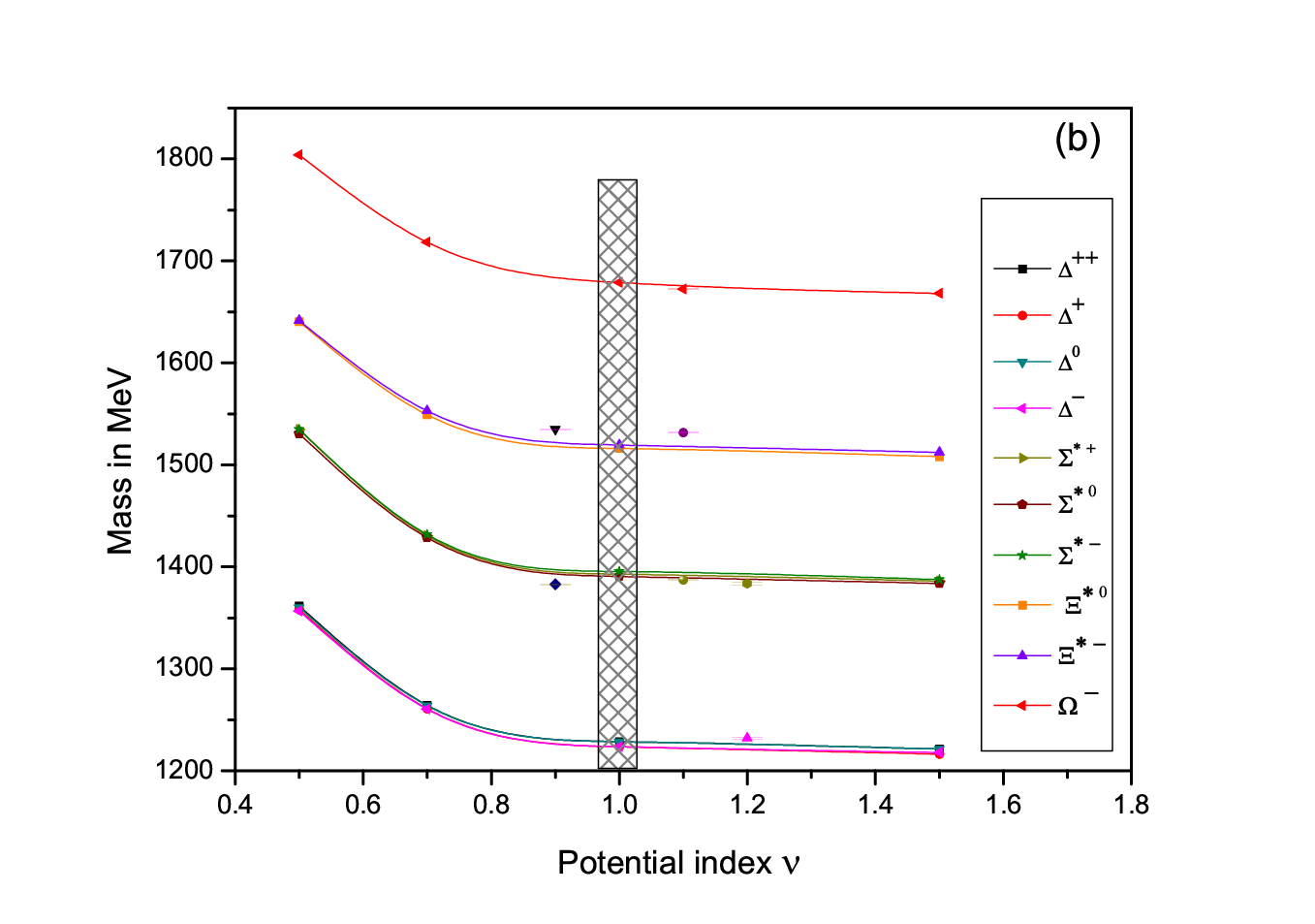
of potential index have been studied. Fig.(1) and
Fig.(2) show the behaviour of the predicted masses of the
octet and decuplet baryons with the potential index in the
range, 0.5 1.5. The trend lines here show saturation
of the masses beyond 1.0. The shaded regions in
Fig.(1) and in Fig.(2) show the neighbour hood
region of at which the predicted masses are having
minimum root mean square deviation with the experimental masses.
The computed magnetic moments of the octet and decuplet baryons are
compared with the known experimental results as well as with other
model predictions in Table 3 and 4 respectively.
Present results for the choice of 0.7 are found to be
in agreement with the known experimental values as well as with
other model predictions. Here, it should be noted that the better
agreement occur for the choice of ()
slightly below the saturation region () (See Fig.1 - 4). However the experimental measurements of
decuplet states are difficult and the known values for the
- baryons carry large errors [1, 2, 3].
The available experimental results for the are
4.50.95 and 3.5-7.5 are in very good agreement with our
calculated magnetic moment 4.52 at = 0.7. The calculated
magnetic moments for , , and are
also in good agreement with experimental result while comparing with
other theoretical models.
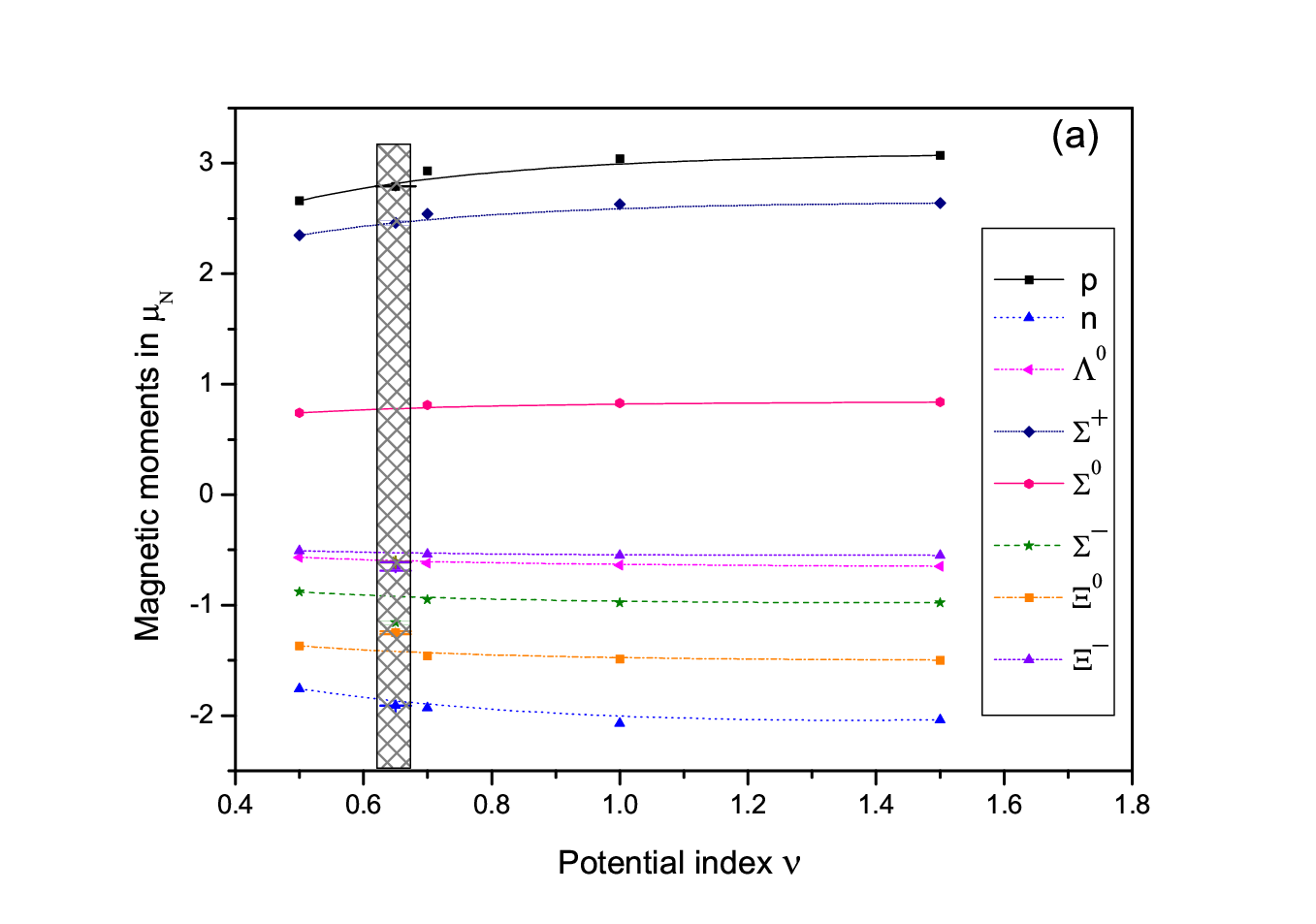
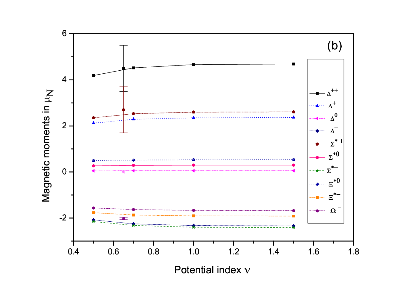
The behavior of the predicted magnetic moments of octet and decuplet
baryons with potential index are shown in Fig.(3)
and Fig.(4) respectively. The same saturation trends
towards saturation beyond the potential index 1.0 are observed. The shaded region in Fig.(3) corresponds to
the region of for which the predicted octet
baryon magnetic moments show minimum root mean square deviation with
the experiments. The predicted magnetic moments of the decuplet
baryons in the same region of are found to be
closer to the existing experimental values of and
baryons.
As the octet magnetic moments are known experimentally, we calculate
the percentage variations of the different model predictions with
respect to the experimental values and are given in Table
7 for comparison. The present
prediction for p, n, , baryons are much better
with lesser percentage error compared to other model predictions.
And the average percentage variations from proton to
obtained from the Table 7 is about only, while
that for the lattice predictions and that of PT predictions is
about and respectively. It can also be seen that the
predictions of QCDSR and PQM are having lower
variations of about 4 only.
The transition magnetic moments obtained from the present study
( model) are in accordance with other theoretical
predictions with much less variations with the choices of . However the experimentally known value for the transition magnetic
moments of (3.23) is
higher than theoretical model predictions (see Table 5).
The parameter free predictions of the radiative decay width for
(N=n,p) transitions obtained here are
in very good agreement with experiment compared to other model
predictions (see Table 6). Prediction for other decuplet to
octet radiative transitions are well within the experimental
limits.
At the end, we like to point out important feature of the
model is the saturation behaviour of the predicted properties of the
baryons with . Similar saturation behaviour was also
observed in the mass predictions of the model in the
heavy flavour sector [33].
It thus suggests that model can adequately
represents the three body interactions among the quarks constituting
the baryons.
Acknowledgement: The authors acknowledge the financial
support from the University Grant commission, Government of India
under a Major research project F. 32-31/2006 (SR).
References
References
- [1] Amsler C et al. (Particle Data Group), Phys. Lett. B 667, 1 (2008).
- [2] M. Kotulla et al. Phys. Rev. Lett. 89, 272001 (1991).
- [3] A. Bosshard et al., Phys. Rev D 44, 1962 (1991).
- [4] W. M. Yao et al. (Particle Data Group), J. Phys. G 33, 1 (2006) and references therein.
- [5] D. B. Leinweber et al. Phys. Rev D 48, 2230 (1993).
- [6] E. Kaxiras et al. Phys. Rev D 32, 695 (1985) and references therein.
- [7] S. Capstick, Phys. Rev D 46, 1965 (1992).
- [8] M. N. Butler, M. J. Savage, and R. P. Springer, Nucl. Phys. B 399, 69 (1993).
- [9] T. M. Aliev and A. Ozpineci, Nucl. Phys. B 732, 291 (2006).
- [10] T. M. Aliev, K. Azizi and A. Ozpineci, Phys. Rev D 79, 056005 (2009).
- [11] M. Bagchi, S. Daw, M. Dey, and J. Dey, Europhys. Lett.,75, 548 (2006).
- [12] T. M. Aliev and A. Ozpineci, Phys. Rev D 62, 053012 (2000).
- [13] Frank X. Lee, Phys. Rev D 57, 1801 (1998).
- [14] D. B. Leinweber, T. Draper, and R. M. Woloshyn , Phys. Rev. D 46, 3067 (1992).
- [15] I. C. Cloet, D. B. Leinweber and A. W. Thomas, Phys. Lett. B 563, 157 (2003).
- [16] I. C. Cloet, D. B. Leinweber and A. W. Thomas, arXiv:nucl-th/0211027
- [17] L. S. Geng, J. Martin Camalich, and M. J. Vicente Vacas, Chinese Physics C 33, X (2009); [arXiv:hep-ph/1001.0465].
- [18] M. N. Butler, M. J. Savage, and R. P. Springer, Phys. Rev. D 49, 3459 (1994).
- [19] Meissner and S. Steininger, Nucl. Phys. B 499, 349 (1997).
- [20] P. Ha and L. Durand, Phys. Rev. D 58, 093008 (1998).
- [21] S. J. Puglia and M. J. Ramsay, Phys. Rev. D 62, 034010 (2000).
- [22] F. Schlumpf, Phys. Rev. D 48, 4478 (1993).
- [23] K. T. Chao, Phys. Rev. D 41, 920 (1990).
- [24] Ha P. and Durand L., Phys. Rev. D 58, 093008 (1998).
- [25] Frank X. Lee, Phys. Lett. B 419, 14 (1998).
- [26] Lai Wang and Frank X. Lee, Phys. Rev. D 78, 013003 (2008).
- [27] H. C. Kim, M. Praszalowicz, and K. Goeke, Phys. Rev. D 57, 2859 (1998).
- [28] H. C. Kim, M. Praszalowicz, Phys. Lett. B 585, 99 (2004).
- [29] Harleen Dahiya, Neetika Sharma and P. K. Chatley [arXiv:hep-ph/0912.5256v1].
- [30] S. T. Hong and G. E. Brown, Nucl. Phys. A 580,408 (1994).
- [31] M. I. Krivoruchenko, Sov. J., Nucl. Phys. A 45,109 (1987).
- [32] Leinweber D. B., Draper T. and Woloshyn R. M., Phys. Rev. D 46, 3067 (1992).
- [33] Patel B, Rai A. K. and Vinodkumar P C, J. Phys. G, 35, 065001 (2008).
- [34] Patel B, Majethiya A and Vinodkumar P C, Pramana - J. Phys. 72, 679 (2009).
- [35] N.Isgur and G. Karl, Phys. Rev. D 18, 4187 (1978); 2653(1979); D 20, 1191 (1979); Phys. Lett. B 72, 109 (1977); Phys. Lett. B 74, 353 (1978).
- [36] S. Godfrey et al., Phys. Rev. D 32, 189 (1985).
- [37] S. Capstick and N. Isgur, Phys. Rev. D 34, 2809 (1986).
- [38] H. Dahiya and M. Gupta, Phys. Rev. D 67, 114015 (2003); M. Gupta anf Navjot Kaur,Phys. Rev. D 28, 534 (1983); J. Singh and M. Gupta, J. Phys. G 16, L 45 (1990).
- [39] M. V. N. Murthy, Z. Phys. C-Particles and Fields 31, 81-86 (1986).
- [40] W. Roberts and M. Pervin, [arXiv:hep-ph/0711.2492v1].
- [41] H Garcilazo, J Vijande and A Valcarce, J. Phys. G 34, 961-976 (2007).
- [42] R. Bijker, F. Iachello and A. Leviatan, Annals of Physics 284, 89-133 (2000).
- [43] E. Santopinto, F. lachello and M. M. Giannini, Eur. Phys. J. A 1, 307- 315 (1998).
- [44] Majethiya A, Patel B, and P C Vinodkumar, Eur. Phys. J A 42, 213 (2009).
- [45] Sameer M. Ikhdair and Ramazan Sever, Int. Jn. Mod. Phys. A 21, 3989 (2006); 18, 4215 (2003); 19, 1771 (2004); 21, 2190 (2006).
- [46] K. Heikkila, N. A. Tornquist and S. Ono, Phys. Rev. D 29, 110 (1984).
- [47] X. T. Song, J. Phys. G 17, 49 (1991).
- [48] J. G. Contreras, R. Huerta, and L. R. Quintero, Revista Mexicana de Fisica 50, 490 (2004).
- [49] Rohit Dhir and R. C. Verma, Eur. Phys. J A 42, 243 (2009).
- [50] Lang Yu et al. Phys. Rev. D 66, 033010 (2002) and references therein.
- [51] Phuoc Ha , J.Phys. G 35, 075006 (2008).
- [52] Mariaaline B. Do Vale et al., Revista brasileira de Fisica 16, 4 (1986).
- [53] J. Franklin, Phys. Rev. D 73, 114001 (2006).
- [54] Bae M. and McGovern J. A., J. Phys. G 22, 199 (1996).
- [55] S.K.Gupta and S.B.Khadkikar, Phys. Rev. D 36, 307 (1987).
- [56] Dai J., Dashen R., Jenkins E. and Manohar A. V., Phys. Rev. D 53, 273 (1996).
- [57] B. O. Kerbikov and Yu. A. Simonov, Phys. Rev. D 62, 093016 (2000).
- [58] J. W. Bos et al. Chinese J. of Phys. 35, 2 (1997).
- [59] K. Azizi, Eur. Phys. J C 61, 311 (2009).
- [60] Lang Yu et al., Phys. Rev. D 73, 114001 (2006).
- [61] S. T. Hong, Phys. Rev. D 76, 094029 (2007).
- [62] S. Eidelman et al., Phys. Lett. B 592, 1 (2004).
- [63] J. Colas et al., Nucl. Phys. B 91, 253 (1975).
- [64] T. S. Mast et al., Phys. Rev. Lett. 21, 1715 (1968).
- [65] V. V. Molchanov et al., Phys. Lett. B 590, 161 (2004).