Optical Integral and Sum Rule Violation

In BCS theory the quantity $Z(\omega)$ is given by

and

This is consistent with having in the NS, $\Sigma=i\Gamma$ in accordance with Eq 6. In the SCS, $\Sigma(\omega)$ is purely imaginary for $\omega>\Delta$ and purely real for $\omega<\Delta$. The self-energy has a square-root singularity at $\omega=\Delta$.

It is worth noting that Eq.12 is derived from the integration over infinite band. If one uses Eq.6 for finite band, Eq.12 acquires an additional frequency dependence at large frequencies of the order of bandwidth (the low frequency structure still remains the same as in Eq.12). In principle, in a fully self-consistent analysis, one should indeed evaluate the self-energy using a finite bandwidth. In practice, however, the self-energy at frequencies of order bandwidth is generally much smaller than $\omega$ and contribute very little to optical conductivity which predominantly comes from frequencies where the self-energy is comparable or even larger than $\omega$. Keeping this in mind, below we will continue with the form of self-energy derived form infinite band. We use the same argument for all four models for the self-energy.

For completeness, we first present some well known results about the conductivity and optical integral for a constant DOS and then extend the discussion to the case where the same calculations are done in the presence of a particular lattice dispersion.

For a constant DOS, $\Delta W(\omega_{c})=W_{SC}(\omega_{c})-W_{NS}(\omega_{c})$ is zero at $\omega_{c}=\infty$ and Kubo sum rule reduces to FGT sum rule. In Fig. 3 we plot for this case $\Delta W(\omega_{c})$ as a function of the cutoff $\omega_{c}$ for different $\Gamma^{\prime}s$. The plot shows the two well known features: zero-crossing point is below $2\Delta$ in the clean limit $\Gamma<<\Delta$ and is roughly $2\Gamma$ in the dirty limit [40, 21] The magnitude of the ‘dip’ decreases quite rapidly with increasing $\Gamma$. Still, there is always a point of zero crossing and $\Delta W({\omega}_{c})$ at large ${\omega}_{c}$ approaches zero from below.

We now perform the same calculations in the presence of lattice dispersion. The results are summarized in Figs 4,5, and 6.

Fig 4 shows conductivities $\sigma(\omega)$ in the NS and the SCS and Kubo sums $W_{K}$ plotted against impurity scattering $\Gamma$. We see that the optical integral in the NS is always greater than in the SCS. The negative sign of $\Delta W_{K}$ is simply the consequence of the fact that $n_{k}$ is larger in the NS for $\epsilon_{k}<0$ and smaller for $\epsilon_{k}<0$, and $\nabla^{2}\varepsilon_{\vec{k}}$ closely follows $-\varepsilon_{\vec{k}}$ for our choice of dispersion [38]), Hence $n_{k}$ is larger in the NS for $\nabla^{2}\varepsilon_{\vec{k}}>0$ and smaller for $\nabla^{2}\varepsilon_{\vec{k}}<0$ and the Kubo sum rule, which is the integral of the product of $n_{k}$ and $\nabla^{2}\varepsilon_{\vec{k}}$ (Eq. 3), is larger in the normal state.

We also see from Fig. 4 that $\Delta W_{K}$ decreases with $\Gamma$ reflecting the fact that with too much impurity scattering there is little difference in $n_{k}$ between NS and SCS.

Fig 5 shows the optical sum in NS and SCS in clean and dirty limits (the parameters are stated in the figure). This plot shows that the Kubo sums are almost completely recovered by integrating up to the bandwidth of $1eV$: the recovery is $95\%$ in the clean limit and $\thicksim 90\%$ in the dirty limit. In Fig 6 we plot $\Delta W({\omega}_{c})$ as a function of ${\omega}_{c}$ in clean and dirty limits. $\Delta W(\infty)$ is now non-zero, in agreement with Fig. 4 and we also see that there is little variation of $\Delta W(\omega_{c})$ at above $0.1-0.3eV$ what implies that for larger ${\omega}_{c}$, $\Delta W({\omega}_{c})\approx\Delta W_{K}>>\Delta f({\omega}_{c})$.

To make this more quantitative, we compare in Fig. 6 $\Delta W({\omega}_{c})$ obtained for a constant DOS, when $\Delta W({\omega}_{c})=\Delta f({\omega}_{c})$, and for the actual lattice dispersion, when $\Delta W({\omega}_{c})=\Delta W_{K}+\Delta f({\omega}_{c})$. In the clean limit there is obviously little cutoff dependence beyond $0.1eV$, i.e., $\Delta f({\omega}_{c})$ is truly small, and the difference between the two cases is just $\Delta W_{K}$. In the dirty limit, the situation is similar, but there is obviously more variation with $\omega_{c}$, and $\Delta f({\omega}_{c})$ becomes truly small only above $0.3eV$. Note also that the position of the dip in $\Delta W({\omega}_{c})$ in the clean limit is at a larger ${\omega}_{c}$ in the presence of the lattice than in a continuum.

We next consider the case of electrons interacting with a single boson mode which by itself is not affected by superconductivity. The primary candidate for such mode is an optical phonon. The imaginary part of the NS self energy has been discussed numerous times in the literature. We make one simplifying assumption – approximate the DOS by a constant in calculating fermionic self-energy. We will, however, keep the full lattice dispersion in the calculations of the optical integral. The advantage of this approximation is that the self-energy can be computed analytically. The full self-energy obtained with the lattice dispersion is more involved and can only be obtained numerically, but its structure is quite similar to the one obtained with a constant DOS.

The self-energy for a constant DOS is given by

where

and $\lambda_{n}$ is a dimensionless electron-boson coupling. Integrating and transforming to real frequencies, we obtain

In the SCS, we obtain for $\omega<0$

Observe that $\Sigma^{\prime\prime}(\omega)$ is no-zero only for $\omega\,<\,-\omega_{o}-\Delta$. Also, although it does not straightforwardly follow from Eq. 16, but real and imaginary parts of the self-energy do satisfy $\Sigma^{\prime}(\omega)=-\Sigma^{\prime}(-\omega)$ and $\Sigma^{\prime\prime}(\omega)=\Sigma^{\prime\prime}(-\omega)$.

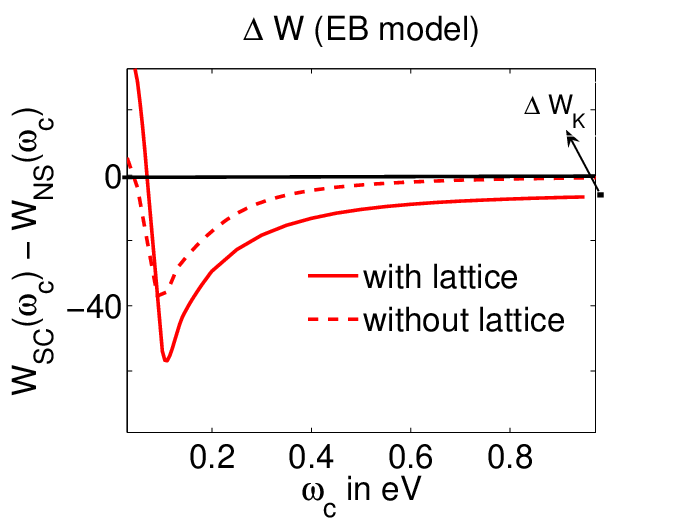
Fig7 shows conductivities $\sigma(\omega)$ and Kubo sums $W_{K}$ as a function of the dimensionless coupling $\lambda$. We see that, like in the previous case, the Kubo sum in the NS is larger than that in the SCS. The difference $\Delta W_{K}$ is between 5 and 8 meV.

Fig 8 shows the evolution of the optical integrals. Here we see the difference with the BCSI model – only about $75\%$ of the optical integral is recovered, both in the NS and SCS, when we integrate up to the bandwidth of $1eV$. The rest comes from higher frequencies.

In Fig 9 we plot $\Delta W({\omega}_{c})$ as a function of ${\omega}_{c}$. We see the same behavior as in the BCSI model in a clean limit – $\Delta W({\omega}_{c})$ is positive at small frequencies, crosses zero at some ${\omega}_{c}$, passes through a deep minimum at a larger frequency, and eventually saturates at a negative value at the largest $w_{c}$. However, in distinction to BCSI model, $\Delta W({\omega}_{c})$ keeps varying with ${\omega}_{c}$ up a much larger scale and saturates only at around $0.8eV$. In between the dip at $0.1eV$ and $0.8eV$, the behavior of the optical integral is predominantly determined by the variation of the cut-off term $\Delta f({\omega}_{c})$ as evidenced by a close similarity between the behavior of the actual $\Delta W$ and $\Delta W$ in the absence of the lattice (the dashed line in Fig. 9).

For their analysis of the optical integral, Norman and Pépin [30] introduced a phenomenological model for the self energy which fits normal state scattering rate measurements by ARPES[41]. It constructs the NS $\Sigma^{{}^{\prime\prime}}(\omega)$ out of two contributions - impurity scattering and electron-electron scattering which they approximated phenomenologically by the marginal Fermi liquid form of $\alpha\omega$ at small frequencies [6] (MFLI model). The total $\Sigma^{{}^{\prime\prime}}$ is

where $\omega_{sat}$ is about $\thicksim\frac{1}{2}$ of the bandwidth, and $f(x)\approx 1$ for $x<1$ and decreases for $x>1$. In Ref 30 $f(x)$ was assumed to scale as $1/x$ at large $x$ such that $\Sigma^{\prime\prime}$ is flat at large $\omega$. The real part of $\Sigma(\omega)$ is obtained from Kramers-Krönig relations. For the superconducting state, they obtained $\Sigma^{{}^{\prime\prime}}$ by cutting off the NS expression on the lower end at some frequency $\omega_{1}$ (the analog of $\omega_{0}+\Delta$ that we had for EB model):

where $\Theta(x)$ is the step function. In reality, $\Sigma^{{}^{\prime\prime}}$ which fits ARPES in the NS has some angular dependence along the Fermi surface [42], but this was ignored for simplicity. This model had gained a lot of attention as it predicted the optical sum in the SCS to be larger than in the NS, i.e., $\Delta W>0$ at large frequencies. This would be consistent with the experimental findings in Refs. 8, 9 if, indeed, one identifies $\Delta W$ measured up to 1eV with $\Delta W_{K}$.

We will show below that the sign of $\Delta W$ in the MFLI model actually depends on how the normal state results are extended to the superconducting state and, moreover, will argue that $\Delta W_{K}$ is actually negative if the extension is done such that at $\alpha=0$ the results are consistent with BCSI model. However, before that, we show in Figs 10-12 the conductivities and the optical integrals for the original MFLI model.

In Fig 10 we plot the conductivities in the NS and the SCS and Kubo sums $W_{K}$ vs $\Gamma$ at $\alpha=0.75$ showing that the spectral weight in the SCS is indeed larger than in the NS. In Fig 11 we show the behavior of the optical sums $W({\omega}_{c})$ in NS and SCS. The observation here is that only $\sim 75-80\%$ of the Kubo sum is recovered up to the scale of the bandwidth implying that there is indeed a significant spectral weight well beyond the bandwidth. And in Fig 12 we show the behavior of $\Delta W(w_{c})$. We see that it does not change sign and remain positive at all ${\omega}_{c}$, very much unlike the BCS case. Comparing the behavior of $W(w_{c})$ with and without a lattice (solid and dashed lines in Fig. 12) we see that the ‘finite bandwidth effect’ just shifts the curve in the positive direction. We also see that the solid line flattens above roughly half of the bandwidth, i.e., at these frequencies $\Delta W({\omega}_{c})\approx\Delta W_{K}$. Still, we found that $\Delta W$ continues going down even above the bandwidth and truly saturates only at about $2\,eV$ (not shown in the figure) supporting the idea that there is ‘more’ left to recover from higher frequencies.

The rationale for $\Delta W_{K}>0$ in the original MFLI model has been provided in Ref. 30. They argued that this is closely linked to the absence of quasiparticle peaks in the NS and their restoration in the SCS state because the phase space for quasiparticle scattering at low energies is smaller in a superconductor than in a normal state. This clearly affects $n_{k}$ because it is expressed via the full Green’s function and competes with the conventional effect of the gap opening. The distribution function from this model, which we show in Fig.2b brings this point out by showing that in a MFLI model, at $\epsilon<0$, $n_{k}$ in a superconductor is larger than $n_{k}$ in the normal state, in clear difference with the BCSI case.

We analyzed the original MFLI model for various parameters and found that the behavior presented in Fig. 12, where $\Delta W({\omega}_{c})>0$ for all frequencies, is typical but not not a generic one. There exists a range of parameters $\alpha$ and $\Gamma$ where $\Delta W_{K}$ is still positive, but $\Delta W({\omega}_{c})$ changes the sign twice and is negative at intermediate frequencies. We show an example of such behavior in Fig14. Still, for most of the parameters, the behavior of $\Delta W({\omega}_{c})$ is the same as in Fig. 12.

On more careful looking we found the problem with the original MFLI model. We recall that in this model the self-energy in the SCS state was obtained by just cutting the NS self energy at $\omega_{1}$ (see Eq.18). We argue that this phenomenological formalism is not fully consistent, at least for small $\alpha$. Indeed, for $\alpha=0$, the MFLI model reduces to BCSI model for which the behavior of the self-energy is given by Eq. (12). This self-energy evolves with $\omega$ and $\Sigma^{{}^{\prime\prime}}$ has a square-root singularity at $\omega=\Delta+\omega_{o}$ (with $\omega_{o}=0$). Meanwhile $\Sigma^{{}^{\prime\prime}}$ in the original MFLI model in Eq. (18) simply jumps to zero at $\omega=\omega_{1}=\Delta$, and this happens for all values of $\alpha$ including $\alpha=0$ where the MFLI and BCSI model should merge. This inconsistency is reflected in Fig 13, where we plot the near-BCS limit of MFLI model by taking a very small $\alpha=0.05$. We see that the optical integral $W_{K}$ in the SCS still remains larger than in the NS over a wide range of $\Gamma$, in clear difference with the exactly known behavior in the BCSI model, where $W_{K}$ is larger in the NS for all $\Gamma$ (see Fig. 4). In other words, the original MFLI model does not have the BCSI theory as its limiting case.

We modified the MFLI model is a minimal way by changing the damping term in a SCS to $\frac{\Gamma}{\sqrt{-\omega^{2}+\Delta^{2}}}$ to be consistent with BCSI model. We still use Eq. (18) for the MFL term simply because this term was introduced in the NS on phenomenological grounds and there is no way to guess how it gets modified in the SCS state without first deriving the normal state self-energy microscopically (this is what we will do in the next section). The results of the calculations for the modified MFLI model are presented in Figs. 15 and 16. We clearly see that the behavior is now different and $\Delta W_{K}<0$ for all $\Gamma$. This is the same behavior as we previously found in BCSI and EB models. So we argue that the ‘unconventional’ behavior exhibited by the original MFLI model is most likely the manifestation of a particular modeling inconsistency. Still, Ref. 30 made a valid point that the fact that quasiparticles behave more close to free fermions in a SCS than in a NS, and this effect tends to reverse the signs of $\Delta W_{K}$ and of the kinetic energy  [43]. It just happens that in a modified MFLI model the optical integral is still larger in the NS.

We now turn to a more microscopic model- the CB model. The model describes fermions interacting by exchanging soft, overdamped collective bosons in a particular, near-critical, spin or charge channel [45, 31, 44]. This interaction is responsible for the normal state self-energy and also gives rise to a superconductivity. A peculiar feature of the CB model is that the propagator of a collective boson changes below $T_{c}$ because this boson is not an independent degree of freedom (as in EB model) but is made out of low-energy fermions which are affected by superconductivity [32].

The most relevant point for our discussion is that this model contains the physics which we identified above as a source of a potential sign change of $\Delta W_{K}$. Namely, at strong coupling the fermionic self-energy in the NS is large because there exists strong scattering between low-energy fermions mediated by low-energy collective bosons. In the SCS, the density of low-energy fermions drops and a continuum collective excitations becomes gaped. Both effects reduce fermionic damping and lead to the increase of $W_{K}$ in a SCS. If this increase exceeds a conventional loss of $W_{K}$ due to a gap opening, the total $\Delta W_{K}$ may become positive.

The CB model has been applied numerous times to the cuprates, most often under the assumption that near-critical collective excitations are spin fluctuations with momenta near $Q=(\pi,\pi)$. This version of a CB boson is commonly known as a spin-fermion model. This model yields $d_{x^{2}-y^{2}}$ superconductivity and explains in a quantitative way a number of measured electronic features of the cuprates, in particular the near-absence of the quasiparticle peak in the NS of optimally doped and underdoped cuprates[39] and the peak-dip-hump structure in the ARPES profile in the SCS[46, 32, 31, 47]. In our analysis we assume that a CB is a spin fluctuation.

The results for the conductivity within a spin-fermion model depend in quantitative (but not qualitative) way on the assumption for the momentum dispersion of a collective boson. This momentum dependence comes from high-energy fermions and is an input for the low-energy theory. Below we follow Refs. 33, 31 and assume that the momentum dependence of a collective boson is flat near $(\pi,\pi)$. The self energy within such model has been worked out consistently in Ref. 33, 31. In the normal state

where $\lambda_{n}$ is the spin-fermion coupling constant, and $\omega_{sf}$ is a typical spin relaxation frequency of overdamped spin collective excitations with a propagator

where $\chi_{Q}$ is the uniform static susceptibility. If we use Ornstein-Zernike form of $\chi(q)$ and use either Eliashberg  [45] or FLEX computational schemes [48], we get rather similar behavior of $\Sigma$ as a function of frequency and rather similar behavior of optical integrals.

The collective nature of spin fluctuations is reflected in the fact that the coupling $\lambda$ and the bosonic frequency $\omega_{sf}$ are related: $\lambda$ scales as $\xi^{2}$, where $\xi$ is the bosonic mass (the distance to a bosonic instability), and $\omega_{sf}\propto\xi^{-2}$ (see Ref. 49). For a flat $\chi(q\sim Q)$ the product $\lambda\omega_{sf}$ does not depend on $\xi$ and is the overall dimensional scale for boson-mediated interactions.

In the SCS fermionic excitations acquire a gap. This gap affects fermionic self-energy in two ways: directly, via the change of the dispersion of an intermediate boson in the exchange process involving a CB, and indirectly, via the change of the propagator of a CB. We remind ourselves that the dynamics of a CB comes from a particle-hole bubble which is indeed affected by $\Delta$.

The effect of a $d-$wave pairing gap on a CB has been discussed in a number of papers, most recently in [31]. In a SCS a gapless continuum described by Eq. (20) transforms into a gaped continuum, with a gap about $2\Delta$ and a resonance at $\omega=\omega_{0}<2\Delta$, where for a $d-$wave gap we define $\Delta$ as a maximum of a $d-$wave gap.

The spin susceptibility near $(\pi,\pi)$ in a superconductor can generally be written up as

where $\Pi$ is evaluated by adding up the bubbles made out of two normal and two anomalous Green’s functions. Below $2\Delta$, $\Pi(\Omega)$ is real ($\sim\Omega^{2}/\Delta$ for small $\Omega$), and the resonance emerges at $\Omega=\omega_{0}$ at which $\Pi(\omega_{0})=\omega_{sf}$. At frequencies larger than $2\Delta$, $\Pi(\Omega)$ has an imaginary part, and this gives rise to a gaped continuum in $\chi(\Omega)$.

The imaginary part of the spin susceptibility around the resonance frequency $\omega_{0}$ is [31]

where $Z_{o}\sim 2\,\omega_{sf}\chi_{0}/\frac{\partial\Pi}{\partial\omega}_{|\Omega=\omega_{0}}$ . The imaginary part of the spin susceptibility describing a gaped continuum exists for for $\Omega\geq 2\Delta$ and is

In Eq. (23) $D(x)=\frac{K_{1}(x)-K_{2}(x)}{x}$, and $K_{1}(x)$ and $K_{2}(x)$ are Elliptic integrals of first and second kind. The real part of $\chi$ is obtained by Kramers-Krönig transform of the imaginary part.

Substituting Eq 6 for $\chi(q,\Omega)$ into the formula for the self-energy one obtains $\Sigma^{\prime\prime}(\omega)$ in a SCS state as a sum of two terms [31]

where,

comes from the interaction with the resonance and

comes from the interaction with the gaped continuum. The real part of $\Sigma$ is obtained by Kramers-Krönig transform of the imaginary part.

We performed the same calculations of conductivities and optical integrals as in the previous three cases. The results are summarized in Figs. 17 - 22. Fig 17 shows conductivities in the NS and the SCS for two couplings $\lambda=1$ and $\lambda=10$ (keeping $\lambda\omega_{sf}$ constant). Other parameters $Z_{o}$ and $\omega_{o}$ are calculated according to the discussion after Eq 21. for $\omega_{sf}=26\,meV$, $\lambda=1$, we find $\omega_{o}=40\,meV$, $Z_{o}=0.77$. And for $\omega_{sf}=2.6\,meV$, $\lambda=10$, we find $\omega_{o}=13.5\,meV$, $Z_{o}=1.22$. Note that the conductivity in the SCS starts at $2\Delta+\omega_{o}$ (i.e. the resonance energy shows up in the optical gap), where as in the BCSI case it would have always begun from $2\Delta$. In Fig 18 we plot the Kubo sums $W_{K}$ vs coupling $\lambda$. We see that for all $\lambda$, $W_{K}$ in the NS stays larger than in the SCS. Fig 19 shows the cutoff dependence of the optical integrals $W({\omega}_{c})$ for $\lambda=1$ separately in the NS and the SCS. We again see that only about $73\%$ of the Kubo sum is recovered up to the bandwidth of $1\,eV$ indicating that there is a significant amount left to recover beyond this energy scale. Fig 20 shows $\Delta W$ for the two different couplings. We see that, for both $\lambda$’s, there is only one zero-crossing for the $\Delta W$ curve, and $\Delta W$ is negative at larger frequencies. The only difference between the two plots is that for larger coupling the dip in $\Delta W$ gets ‘shallower’. Observe also that the solid line in Fig. 20 is rather far away from the dashed line at $\omega_{c}>1meV$, which indicates that, although $\Delta W({\omega}_{c})$ in this region has some dependence on ${\omega}_{c}$, still the largest part of $\Delta W({\omega}_{c})$ is $\Delta W_{K}$, while the contribution from $\Delta f(\omega_{c})$ is smaller.

The negative sign of $\Delta W({\omega}_{c})$ above a relatively small $\omega_{c}\sim 0.1-0.2eV$ implies that the ‘compensating’ effect from the fermionic self-energy on $\Delta W$ is not strong enough to overshadow the decrease of the optical integral in the SCS due to gap opening. In other words,the CB model displays the same behavior as BCSI, EB, and modified MFLI models. It is interesting that this holds despite the fact that for large $\lambda$ CB model displays the physics one apparently needs to reverse the sign of $\Delta W_{K}$ – the absence of the quasiparticle peak in the NS and its emergence in the SCS accompanied by the dip and the hump at larger energies. The absence of coherent quasiparticle in the NS at large $\lambda$ is also apparent form Fig 21 where we show the normal state distribution functions for two different $\lambda$. For large $\lambda$ the jump (which indicates the presence of quasiparticles) virtually disappears.

On a more careful look, we found that indifference of $\delta W({\omega}_{c})$ to the increase of $\lambda$ is merely the consequence of the fact that above we kept $\lambda\omega_{sf}$ constant. Indeed, at small frequencies, fermionic self-energy in the NS is $\Sigma^{\prime}=\lambda\omega$, $\Sigma"=\lambda^{2}\omega^{2}/(\lambda\omega_{sf})$, and both $\Sigma^{\prime}$ and $\Sigma^{\prime\prime}$ increase with $\lambda$ if we keep $\lambda\omega_{sf}$ constant. But at frequencies larger than $\omega_{sf}$, which we actually probe by $\Delta W({\omega}_{c})$, the self-energy essentially depends only on $\lambda\omega_{sf}$, and increasing $\lambda$ but keeping $\lambda\omega_{sf}$ constant does not bring us closer to the physics associated with the recovery of electron coherence in the SCS. To detect this physics, we need to see how things evolve when we increase $\lambda\omega_{sf}$ above the scale of $\Delta$ , i.e., consider a truly strong coupling when not only $\lambda\gg 1$ but also the normal state $\Sigma_{NS}(\omega\geq\Delta)>>\Delta$.

To address this issue, we took a larger $\lambda$ for the same $\omega_{sf}$ and re-did the calculation of the conductivities and optical integrals. The results for $\sigma(\omega)$ and $\Delta W({\omega}_{c})$ are presented in Fig. 22. We found the same behavior as before, i.e., $\Delta W_{K}$ is negative. But we also found that the larger is the overall scale for the self-energy, the larger is a frequency of zero-crossing of $\Delta W({\omega}_{c})$. In particular, for the same $\lambda$ and $\omega_{sf}$ that were used in Ref. 33 to fit the NS conductivity data, the zero crossing is at $\sim 0.8\,eV$ which is quite close to the bandwidth. This implies that at a truly strong coupling the frequency at which $\Delta W({\omega}_{c})$ changes sign can well be larger than the bandwidth of $1eV$ in which case $\Delta W$ integrated up to the bandwidth does indeed remain positive. Such behavior would be consistent with Refs.8, 9. we also see from Fig. 22 that $\Delta W_{K}$ becomes small at a truly strong coupling, and over a wide range of frequencies the behavior of $\Delta W({\omega}_{c})$ is predominantly governed by $\Delta f({\omega}_{c})$, i.e. by the cut-off term. [50] The implication is that, to first approximation, $\Delta W_{K}$ can be neglected and positive $\Delta W(w_{c})$ integrated to a frequency where it is still positive is almost compensated by the integral over larger frequencies. This again would be consistent with the experimental data in Refs. 8, 9.

It is also instructive to understand the interplay between the behavior of $\Delta W({\omega}_{c})$ and the behavior of the difference of the kinetic energy between the SCS and the NS, $\delta_{KE}$. We computed the kinetic energy as a function of $\lambda\omega_{sf}$ and present the results in Fig. 23 for $\lambda=1$ and $10$. For a relatively weak $\lambda=1$ the behavior is clearly BCS like- $\delta_{KE}>0$ and increases with increasing $\lambda\omega_{sf}$. However, at large $\lambda=10$, we see that the kinetic energy begin decreasing at large $\lambda\omega_{sf}$ and eventually changes sign. The behavior of $\delta_{KE}$ at a truly strong coupling is consistent with earlier calculation of the kinetic energy for Ornstein-Zernike form of the spin susceptibility [43].

We clearly see that the increase of the zero crossing frequency of $\Delta W({\omega}_{c})$ at a truly strong coupling is correlated with the non-BCS behavior of $\delta_{KE}$. At the same time, the behavior of $\delta W({\omega}_{c})$ is obviously not driven by the kinetic energy as eventually $\delta W({\omega}_{c})$ changes sign and become negative. Rather, the increase in the frequency range where $\Delta W({\omega}_{c})$ remains positive and non-BCS behavior of $\delta_{KE}$ are two indications of the same effect that fermions are incoherent in the NS but acquire coherence in the SCS.

References

- [1] R. Kubo, J. Phys. Soc. Jpn 12, 570(1957).
- [2] R.A. Ferrrel and R.E. Glover, Phys. Rev.109, 1398 (1958).
- [3] M. Tinkham and R.A. Ferrrel, Phys. Rev. Lett. 2, 331 (1959), M. Tinkham, Introduction to Superconductivity (McGraw-Hill, New York, 1975).
- [4] J. Hirsch, Physica C 199, 305 (1992).
- [5] D. N. Basov and T. Timusk, Rev. Mod. Phys. 77, 721 (2005); A. V. Puchkov, D. N. Basov and T. Timusk, J. Phys. Cond. Matter 8, 10049 (1996).
- [6] C. M. Varma et al, Phys. Rev. Lett. 63, 1996 (1989).
- [7] D. N. Basov, S. I. Woods, A. S. Katz, E. J. Singley, R. C. Dynes, M. Xu, D. G. Hinks, C. C. Homes and M. Strongin, Science 283, 49 (1999).
- [8] H.J.A Molegraaf, C. Presura, D. van der Marel, P.H. Kess, M. Li, Science 295, 2239 (2002); A. B. Kuzmenko, H. J. A. Molegraaf, F. Carbone and D. van der Marel, Phys. Rev. B 72, 144503 (2005).
- [9] A. F. Santander-Syro, R. P. S. M. Lobo, N. Bontemps, Z. Konstantinovic, Z. Z. Li and H. Raffy, Europhys. Lett. 62, 568 (2003);
- [10] A. V. Boris, N. N. Kovaleva, O. V. Dolgov, T. Holden, C. T. Lin, B. Keimer and C. Bernhard, Science 304, 708 (2004).
- [11] G. Deutscher, A. F. Santander-Syro and N. Bontemps, Phys. Rev. B 72, 092504 (2005).
- [12] F. Carbone, A. B. Kuzmenko, H. J. A. Molegraaf, E. van Heumen, V. Lukovac, F. Marsiglio, D. van der Marel, K. Haule, G. Kotliar, H. Berger, S. Courjault, P. H. Kes and M. Li, Phys. Rev. B 74, 064510 (2006).
- [13] C. C. Homes, S. V. Dordevic, D. A. Bonn, R. Liang and W. N. Hardy, Phys. Rev. B 69, 024514 (2004).
- [14] J. Hwanget al, Phys. Rev. B 73, 014508 (2006).
- [15] E. van Heumen, R. Lortz, A. B. Kuzmenko, F. Carbone, D. van der Marel, X. Zhao, G. Yu, Y. Cho, N. Barisic, M. Greven, C. C. Homes and S. V. Dordevic, Phys. Rev. B 75, 054522 (2007).
- [16] M. Ortolani, P. Calvani and S. Lupi, Phys. Rev. Lett. 94, 067002 (2005).
- [17] A.F. Santander-Syro, R.P.S.M. Lobo, and N. Bontemps, Phys. Rev. B 70, 134504(2004), A. F. Santander-Syro, R. P. S. M. Lobo, N. Bontemps, Z. Konstantinovic, Z. Z. Li and H. Raffy, Europhys. Lett. 62, 568 (2003).
- [18] P. F. Maldague, Phys. Rev. B 16 2437 (1977); E. H. Kim, Phys. Rev. B 58 2452 (1998).
- [19] J. Hirsch, Physica C, 201, 347 (1992) and Ref 4.
- [20] for a review see F. Marsiglio, J. Superconductivity and Novel Magnetism 22, 269 (2009).
- [21] F. Marsiglio, E. van Heumen, A. B. Kuzmenko, Phys. Rev. B 77 144510 (2008).
- [22] M. R. Norman, A. V. Chubukov, E. van Heumen, A. B. Kuzmenko, and D. van der Marel, Phys. Rev. B 76, 220509 (2007).
- [23] J. E. Hirsch and F. Marsiglio, Physica C 331, 150 (2000) and Phys. Rev. B 62, 15131 (2000).
- [24] A. Toschi, M. Capone, M. Ortolani, P. Calvani, S. Lupi and C. Castellani, Phys. Rev. Lett. 95, 097002 (2005).
- [25] F. Marsiglio, F. Carbone, A. Kuzmenko and D. van der Marel, Phys. Rev. B 74, 174516 (2006).
- [26] L. Benfatto, S. G. Sharapov, N. Andrenacci and H. Beck, Phys. Rev. B 71, 104511 (2005).
- [27] D. van der Marel, H.J.A. Molegraaf, C. Presura, and I. Santoso, Concepts in Electron Correlations, edited by A. Hewson and V. Zlatic (Kluwer, 2003)
- [28] L. Benfatto, J.P. Carbotte and F. Marsiglio, Phys. Rev. B 74, 155115 (2006)
- [29] F. Marsiglio, Phys. Rev. B 73, 064507(2006).
- [30] M.R. Norman and C. Pépin, Phys. Rev. B 66, 100506(R) (2002).
- [31] J. Fink et al., Phys. Rev. B 74, 165102(R) (2006).
- [32] M. Eschrig, Adv. Phys. 55, 47-183 (2006)
- [33] M.R. Norman and A.V. Chubukov, Phys. Rev. B 73, 140501(R)(2006).
- [34] A.E. Karakozov and E.G. Maksimov, cond-mat/0511185, A. E. Karakozov, E. G. Maksimov and O. V. Dolgov, Solid State Comm. 124, 119 (2002); A. E. Karakozov and E. G. Maksimov, ibid. 139, 80 (2006).
- [35] see e.g., P. B. Allen, Phys. Rev. B 3, 305 (1971); S. V. Shulga, O. V. Dolgov and E. G. Maksimov, Physica C 178, 266 (1991).
- [36] A. A. Abriskov and L. P. Gor’kov, JETP 35, 1090 (1959), Sang Boo Nam, Phys. Rev. 156, 470 (1967).
- [37] Theory of superconductivity, Schrieffer, (W. A. Benjamin Inc., New York 1964).
- [38] M.R. Norman, M. Randeria, H. Ding, and J.C. Campuzano, Phys. Rev. B 52, 615 (1995).
- [39] Z.X. Shen and D.S. Dessau, Phys. Rep. 253, 1(1995), J. C. Campuzano, M. R. Norman, and M. Randeria, “Superconductivity”(Vol-1), 923-992, Springer (2008).
- [40] A. V. Chubukov, Ar. Abanov, and D. N. Basov, Phys. Rev. B 68, 024504 (2003).
- [41] T. Valla et al., Phys. Rev. Lett 85, 828(2000).
- [42] Kaminski et al., Phys. Rev. B 71, 014517 (2005).
- [43] Robert Haslinger and Andrey V. Chubukov, Phys. Rev. B 67, 140504(2003).
- [44] C. Castellani, C. DiCastro, and M. Grilli, Phys. Rev. Lett. 75, 4650 (1995).
- [45] Ar. Abanov, A. Chubukov, and J. Schmalian, Adv. Phys. 52, 119 (2003).
- [46] Dessau et al., Phys. Rev. Lett 66, 2160(1991), Norman et al, Phys. Rev. Lett. 79, 3506(1997).
- [47] M.R. Norman and H. Ding, Phys. Rev. B 57, 11089(1998).
- [48] C. Timm, D. Manske and K. H. Bennemann, Phys. Rev. B 66, 094515(2002).
- [49] A.V. Chubukov, M.R. Norman, Phys. Rev. B 70, 174505(2004).
- [50] In this respect, our results are consistent with the analysis of in a system without a lattice (Ref.[51]). The authors of that work also found that the frequency of zero-crossing of increases with the coupling strength.
- [51] Ar. Abanov and A.V. Chubukov, Phys. Rev. B 70, 100504 (2004).