Inference of global clusters from locally distributed data
Abstract
We consider the problem of analyzing the heterogeneity of clustering distributions for multiple groups of observed data, each of which is indexed by a covariate value, and inferring global clusters arising from observations aggregated over the covariate domain. We propose a novel Bayesian nonparametric method reposing on the formalism of spatial modeling and a nested hierarchy of Dirichlet processes. We provide an analysis of the model properties, relating and contrasting the notions of local and global clusters. We also provide an efficient inference algorithm, and demonstrate the utility of our method in several data examples, including the problem of object tracking and a global clustering analysis of functional data where the functional identity information is not available. 11 1 This work was partially supported by NSF-CDI grant No. 0940671. The author wishes to thank the referees and the Associate Editor for valuable comments that help improve the presentation of this work.
XuanLong Nguyen
Department of Statistics
University of Michigan
Keywords: global clustering, local clustering, nonparametric Bayes, hierarchical Dirichlet process, Gaussian process, graphical model, spatial dependence, Markov chain Monte Carlo, model identifiability
1 Introduction
In many applications it is common to separate observed data into groups (populations) indexed by some covariate . A particularly fruitful characterization of grouped data is the use of mixture distributions to describe the populations in terms of clusters of similar behaviors. Viewing observations associated with a group as local data, and the clusters associated with a group as local clusters, it is often of interest to assess how the local heterogeneity is described by the changing values of covariate . Moreover, in some applications the primary interest is to extract some sort of global clustering patterns that arise out of the aggregated observations.
Consider, for instance, a problem of tracking multiple objects moving in a geographical area. Using covariate to index the time point, at a given time point we are provided with a snapshot of the locations of the objects, which tend to be grouped into local clusters. Over time, the objects may switch their local clusters. We are not really interested in the movement of each individual object. It is the paths over which the local clusters evolve that are our primary interest. Such paths are the global clusters. Note that the number of global and local clusters are unknown, and are to be inferred directly from the locally observed groups of data.
The problem of estimating global clustering patterns out of locally observed groups of data also arises in the context of functional data analysis where the functional identity information is not available. By the absence of functional identity information, we mean the data are not actually given as a collection of sampled functional curves (even if such functional curves exist in reality or conceptually), due to confidentiality constraints or the impracticality of matching the identity of individual functional curves. As another example, the progesterone hormone behaviors recorded by a number of women on a given day in their monthly menstrual cycle is associated with a local group, which are clustered into typical behaviors. Such local clusters and the number of clusters may evolve throughout the monthly cycle. Moreover, aggregating the data over days in the cycle, there might exist one or more typical monthly (“global” trend) hormone behaviors due to contraception or medical treatments. These are the global clusters. Due to privacy concern, the subject identity of the hormone levels are neither known nor matched across the time points . In other words, the data are given not as a collection of hormone curves, but as a collection of hormone levels observed over time.
In the foregoing examples, the covariate indexes the time. In other applications, the covariate might index geographical locations where the observations are collected. More generally, observations associated with different groups may also be of different data types. For instance, consider the assets of a number of individuals (or countries), where the observed data can be subdivided into holdings according to different currency types (e.g., USD, gold, bonds). Here, each is associated with a currency type, and a global cluster may be taken to represent a typical portforlio of currency holdings by a given individual. In view of a substantial existing body of work drawing from the spatial statistics literature that we shall describe in the sequel, throughout this paper a covariate value is sometimes referred to as a spatial location unless specified otherwise. Therefore, the dependence on varying covariate values of the local heterogeneity of data is also sometimes referred to as the spatial dependence among groups of data collected at varying local sites.
We propose in this paper a model-based approach to learning global clusters from locally distributed data. Because the number of both global and local clusters are assumed to be unknown, and because the local clusters may vary with the covariate , a natural approach to handling this uncertainty is based on Dirichlet process mixtures and their variants. A Dirichlet process defines a distribution on (random) probability measures, where is called the concentration parameter, and parameter denotes the base probability measure or centering distribution (Ferguson, 1973). A random draw from the Dirichlet process (DP) is a discrete measure (with probability 1), which admits the well-known “stick-breaking” representation (Sethuraman, 1994):
| (1) |
where the ’s are independent random variables distributed according to , denotes an atomic distribution concentrated at , and the stick breaking weights are random and depend only on parameter . Due to the discrete nature of the DP realizations, Dirichlet processes and their variants have become an effective tool in mixture modeling and learning of clustered data. The basic idea is to use the DP as a prior on the mixture components in a mixture model, where each mixture component is associated with an atom in . The posterior distribution of the atoms provides the probability distribution on mixture components, and also yields a probability distribution of partitions of the data. The resultant mixture model, generally known as the Dirichlet process mixture, was pioneered by the work of Antoniak (1974) and subsequentially developed by many others (e.g., (Lo, 1984; Escobar and West, 1995; MacEachern and Mueller, 1998)).
A Dirichlet process (DP) mixture can be utilized to model each group of observations, so a key issue is how to model and assess the local heterogeneity among a collection of DP mixtures. In fact, there is an extensive literature in Bayesian nonparametrics that focuses on coupling multiple Dirichlet process mixture distributions (e.g., MacEachern (1999); Mueller et al. (2004); DeIorio et al. (2004); Ishwaran and James (2001); Teh et al. (2006)). A common theme has been to utilize the Bayesian hierarchical modeling framework, where the parameters are conditionally independent draws from a probability distribution. In particular, suppose that the -indexed group is modeled using a mixing distribution . We highlight the hierarchical Dirichlet process (HDP) introduced by Teh et al. (2006), a framework that we shall subsequentially generalize, which posits that for some base measure and concentration parameter . Moreover, is also random, and is distributed according to another DP: . The HDP model and other aforementioned work are inadequate for our problem, because we are interested in modeling the linkage among the groups not through the exchangeability assumption among the groups, but through the more explicit dependence on changing values of a covariate .
Coupling multiple DP-distributed mixture distributions can be described under a general framework outlined by MacEachern (1999). In this framework, a DP-distributed random measure can be represented by the random “stick” and “atom” random variables (see Eq. (1)), which are general stochastic processes indexed by . Starting from this representation, there are a number of proposals for co-varying infinite mixture models (Duan et al., 2007; Petrone et al., 2009; Rodriguez et al., 2010; Dunson, 2008; Nguyen and Gelfand, 2010). These proposals were designed for functional data only, i.e., where the data are given as a collection of sampled functions of , and thus not suitable for our problem, because functional identity information is assumed unknown in our setting. In this regard, the work of Griffin and Steel (2006); Dunson and Park (2008); Rodriguez and Dunson (2009) are somewhat closer to our setting. These authors introduced spatial dependency of the local DP mixtures through the stick variables in a number of interesting ways, while Rodriguez and Dunson (2009) additionally considered spatially varying atom variables, resulting in a flexible model. These work focused mostly on the problem of interpolation and prediction, not clustering. In particular, they did not consider the problem of inferring global clusters from locally observed data groups, which is our primary goal.
To draw inferences about global clustering patterns from locally grouped data, in this paper we will introduce an explicit notion of and model for global clusters, through which the dependence among locally distributed groups of data can be described. This allows us to not only assess the dependence of local clusters associated with multiple groups of data indexed by , but also to extract the global clusters that arise from the aggregated observations. From the outset, we use a spatial stochastic process, and more generally a graphical model indexed over to characterize the centering distribution of global clusters. Spatial stochastic process and graphical models are versatile and customary choice for modeling of multivariate data (Cressie, 1993; Lauritzen, 1996; Jordan, 2004). To “link” global clusters to local clusters, we appeal to a hierarchical and nonparametric Bayesian formalism: The distribution of global clusters is random and distributed according to a DP: . For each , the distribution of local clusters is assumed random, and is distributed according to a DP: , where denotes the marginal distribution at induced by the stochastic process . In other words, in the first stage, the Dirichlet process provides support for global atoms, which in turn provide support for the local atoms of lower dimensions for multiple groups in the second stage. Due to the use of hierarchy and the discreteness property of the DP realizations, there is sharing of global atoms across the groups. Because different groups may share only disjoint components of the global atoms, the spatial dependency among the groups is induced by the spatial distribution of the global atoms. We shall refer to the described hierarchical specification as the nested Hierarchical Dirichlet process (nHDP) model.
The idea of incorporating spatial dependence in the base measure of Dirichlet processes goes back to Cifarelli and Regazzini (1978); Muliere and Petrone (1993); Gelfand et al. (2005), although not in a fully nonparametric hierarchical framework as is considered here. The proposed nHDP is an instantiation of the nonparametric and hierarchical modeling philosophy eloquently advocated in Teh and Jordan (2010), but there is a crucial distinction: Whereas Teh and Jordan generally advocated for a recursive construction of Bayesian hierarchy, as exemplified by the popular HDP (Teh et al., 2006), the nHDP features a richer nested hierarchy: instead of taking a joint distribution, one can take marginal distributions of a random distribution to be the base measure to a DP in the next stage of the hierarchy. This feature is essential to bring about the relationship between global clusters and local clusters in our model. In fact, the nHDP generalizes the HDP model in the following sense: If places a prior with probability one on constant functions (i.e., if then ) then the nHDP is reduced to the HDP.
Most closely related to our work is the hybrid DP of Petrone et al. (2009), which also considers global and local clustering, and which in fact serves as an inspiration for this work. Because the hybrid DP is designed for functional data, it cannot be applied to situations where functional (curve) identity information is not available, i.e., when the data are not given as a collection of curves. When such functional id information is indeed available, it makes sense to model the behavior of individual curves directly, and this ability may provide an advantage over the nHDP. On the other hand, the hybrid DP is a rather complex model, and in our experiment (see Section 5), it tends to overfit the data due to the model complexity. In fact, we show that the nHDP provides a more satisfactory clustering performance for the global clusters despite not using any functional id information, while the hybrid DP requires not only such information, it also requires the number of global clusters (“pure species”) to be pre-specified. It is worth noting that in the proposed nHDP, by not directly modeling the local cluster switching behavior, our model is significantly simpler from both viewpoints of model complexity and computational efficiency of statistical inference.
The paper outline is as follows. Section 2 provides a brief background of Dirichlet processes, the HDP, and we then proceed to define the nHDP mixture model. Section 3 explores the model properties, including a stick-breaking characterization, an analysis of the underlying graphical and spatial dependency, a Pólya-urn sampling characterization. We also offer a discussion of a rather interesting issue intrinsic to our problem and the solution, namely, the conditions under which global clusters can be identified based on only locally grouped data. As with most nonparametric Bayesian methods, inference is an important issue. We demonstrate in Section 4 that the confluence of graphical/spatial with hierarchical modeling allows for efficient computations of the relevant posterior distributions. Section 5 presents several experimental results, including a comparison to a recent approach in the literature. Section 6 concludes the paper.
2 Model formalization
2.1 Background
We start with a brief background on Dirichlet processes (Ferguson, 1973), and then proceed to hierarchical Dirichlet processes (Teh et al., 2006). Let be a probability space, and . A Dirichlet process is defined to be the distribution of a random probability measure over such that, for any finite measurable partition of , the random vector is distributed as a finite dimensional Dirichlet distribution with parameters . is referred to as the concentration parameter, which governs the amount of variability of around the centering distribution . A DP-distributed probability measure is discrete with probability one. Moreover, it has a constructive representation due to Sethuraman (1994): , where are iid draws from , and denotes an atomic probability measure concentrated at atom . The elements of the sequence are referred to as “stick-breaking” weights, and can be expressed in terms of independent beta variables: , where are iid draws from . Note that satisfies with probability one, and can be viewed as a random probabity measure on the positive integers. For notational convenience, we write , following Pittman (2002).
A useful viewpoint for the Dirichlet process is given by the Pólya urn scheme, which shows that draws from the Dirichlet process are both discrete and exhibit a clustering property. From a computational perspective, the Pólya urn scheme provides a method for sampling from the random distribution , by integrating out . More concretely, let atoms are iid random variables distributed according to . Because is random, are exchangeable. Blackwell and MacQueen (1973) showed that the conditional distribution of given has the following form:
This expression shows that has a positive probability of being equal to one of the previous draws . Moreover, the more often an atom is drawn, the more likely it is to be drawn in the future, suggesting a clustering property induced by the random measure . The induced distribution over random partitions of is also known as the Chinese restaurant process (Aldous, 1985).
A Dirichlet process mixture model utilizes as the prior on the mixture component . Combining with a likelihood function , the DP mixture model is given as: ; . Such mixture models have been studied in the pioneering work of Antoniak (1974) and subsequentially by a number of authors (Lo, 1984; Escobar and West, 1995; MacEachern and Mueller, 1998), For more recent and elegant accounts on the theories and wide-ranging applications of DP mixture modeling, see Hjort et al. (2010).
Hierarchical Dirichlet Processes.
Next, we proceed giving a brief background on the HDP formalism of Teh et al. (2006), which is typically motivated from the setting of grouped data. Under this setting, the observations are organized into groups indexed by a covariate , where is the index set. Let , be the observations associated with group . For each , the are assumed to be exchangeable. This suggests the use of mixture modeling: The are assumed identically and independently drawn from a mixture distribution. Specifically, let denote the parameter specifying the mixture component associated with . Under the HDP formalism, is the same space for all , i.e., for all , and is endowed with the Borel -algebra of subsets of . is referred to as local factors indexed by covariate . Let denote the distribution of observation given the local factor . Let denote a prior distribution for the local factors . We assume that the local factors ’s are conditionally independent given . As a result we have the following specification:
| (2) |
Under the HDP formalism, to statistically couple the collection of mixing distributions , we posit that random probability measures are conditionally independent, with distributions given by a Dirichlet process with base probability measure :
Moreover, the HDP framework takes a fully nonparametric and hierarchical specification, by positing that is also a random probability measure, which is distributed according to another Dirichlet process with concentration parameter and base probability measure :
An interesting property of the HDP is that because ’s are discrete random probability measures (with probability one) whose support are given by the support of . Moreover, is also a discrete measure, thus the collection of are random discrete measures sharing the same countable support. In addition, because the random partitions induced by the collection of within each group are distributed according to a Chinese restaurant process, the collection of these Chinese restaurant processes are statistically coupled. In fact, they are exchangeable, and the distribution for the collection of such stoschastic processes is known as the Chinese restaurant franchise (Teh et al., 2006).
2.2 Nested hierarchy of DPs for global clustering analysis
Setting and notations. In this paper we are interested in the same setting of grouped data as that of the HDP that is described by Eq. (2). Specifically, the observations within each group are iid draws from a mixture distribution. The local factor denotes the parameter specifying the mixture component associated with . The are iid draws from the mixing distribution .
Implicit in the HDP model is the assumptions that the spaces all coincide, and that random distributions are exchangeble. Both assumptions will be relaxed. Moreover, our goal here is the inference of global clusters, which are associated with global factors that lie in the product space . To this end, is endowed with a -algebra to yield a measurable space . Within this paper and in the data illustrations, , and corresponds to the Borel -algebra of subsets of , Formally, a global factor, which are denoted by or in the sequel, is a high dimensional vector (or function) in whose components are indexed by covariate . That is, , and . As a matter of notations, we always use to denote the numbering index for (so we have ). We always use and to denote the number index for instances of ’s and ’s, respectively (e.g., and ). The components of a vector () are denoted by (). We may also use letters and beside to denote the group indices.
Model description.
Our modeling goal is to specify a distribution on the global factors , and to relate to the collection of mixing distributions associated with the groups of data. Such resultant model shall enable us to infer about the global clusters associated with a global factor on the basis of data collected locally by the collection of groups indexed by . At a high level, the random probability measures and the ’s are “glued” together under the nonparametric and hierarchical framework, while the probabilistic linkage among the groups are governed by a stochastic process indexed by and distributed according to . Customary choices of such stochastic processes include either a spatial process, or a graphical model .
Specifically, let denote the induced marginal distribution of . Our model posits that for each , is a random measure distributed as a DP with concentration parameter , and base probability measure : . Conditioning on , the distributions are independent, and varies around the centering distribution , with the amount of variability given by . The probability measure is random, and distributed as a DP with concentration parameter and base probability measure : , where is taken to be a spatial process indexed by , or more generally a graphical model defined on the collection of variables indexed by . In summary, collecting the described specifications gives the nested Hierarchical Dirichlet process (nHDP) mixture model:
As we shall see in the next section, the ’s, which are draws from , provide the support for global factors , which in turn provide the support for the local factors . The global and local factors provide distinct representations for both global clusters and local clusters that we envision being present in data. Local factors ’s provide the support for local cluster centers at each . The global factors in turn provide the support for the local clusters, but they also provide the support for global cluster centers in the data, when observations are aggregated across different groups.
Relations to the HDP.
Both the HDP and nHDP are instances of the nonparametric and hierarchical modeling framework involving hierarchy of Dirichlet processes (Teh and Jordan, 2010). At a high-level, the distinction here is that while the HDP is a recursive hierarchy of random probability measures generally operating on the same probability space, the nHDP features a nested hierarchy, in which the probability spaces associated with different levels in the hierarchy are distinct but related in the following way: the probability distribution associated with a particular level, say , has support in the support of the marginal distribution of a probability distribution (i.e., ) in the upper level in the hierarchy. Accordingly, for , and have support in distinct components of vectors . For a more explicit comparison, it is simple to see that if places distribution for constant global factors with probability one (e.g., for any there holds ), then we obtain the HDP of Teh et al. (2006).
3 Model properties
3.1 Stick-breaking representation and graphical or spatial dependency
Given that the multivariate base measure is distributed as a Dirichlet process, it can be expressed using Sethuraman’s stick-breaking representation: . Each atom is multivariate and denoted by . The ’s are independent draws from , and . The ’s and are mutually independent. The marginal induced by at each location is: . Since each has support at the points , each necessarily has support at these points as well, and can be written as:
| (3) |
Let . Since ’s are independent given , the weights ’s are independent given . Moreover, because it is possible to derive the relationship between weights ’s and . Following Teh et al. (2006), if is non-atomic, it is necessary and sufficient for defined by Eq. (3) to satisfy that the following holds: , where and are interpreted as probability measures on the set of positive integers.
The connection between the nHDP and the HDP of Teh et al. (2006) can be observed clearly here: The stick-breaking weights of the nHDP-distributed have the same distributions as those of the HDP, while the atoms are linked by a graphical model distribution, or more generally a stochastic process indexed by .
The spatial/graphical dependency given by base measure induces the dependency between the DP-distributed ’s. We shall explore this in details by considering specific examples of .
 |
 |
Example 1 (Graphical model ). For concreteness, we consider a graphical model of three variables which are associated with three locations . Moreover, assume the conditional independence relation: . Let be a random draw from . Because , also has distribution once is integrated out. Thus, .
At each location , the marginal distribution of variable is random and . Moreover, in general the ’s are mutually dependent regardless of any (conditional) independence relations that might confer. This fact can be easily seen from Eq. (3). With probability 1, all ’s share the same . It follows that . Because is random, the conditional independence relation no longer holds among in general. From a modeling standpoint, the dependency among the ’s is natural for our purpose, as provides the distribution for the global factors associated with the global clusters that we are also interested in inferring.
Turning now to distributions for local factors , we note that are independent given . Moreover, for each , the support of is the same as that of (i.e., for take value among ). Integrating over the random , for any measurable partition , there holds: . In sum, the global factors ’s take values in the set of , and provide the support set for the local factors ’s at each . The prior means of the local factors ’s are also derived from the prior mean of the global factors.
Example 2 (Spatial model ). To quantify more detailed dependency among DP-distributed ’s, let be a finite subset of and be a second-order stochastic process indexed by . A customary choice for is a Gaussian process. In effect, , where the covariance has entries of the exponential form: .
For any measurable partitions , and , we are interested in expressions for variation and correlation measures under and ’s. Let . Define . Applying stick-breaking representation for , it is simple to derive that:
Proposition 1.
For any pair of distinct locations , there holds:
| (4) | |||||
| (5) | |||||
| (6) | |||||
For any pair of locations , if , it follows that . Due to standard properties of Gaussian variables, and become less dependent of each other, and , so that . On the other hand, if , we obtain that , as desired.
Turning to distributions ’s for the local factors, the following result can be shown:
Proposition 2.
For any pair of , there holds:
| (7) | |||||
where .
Eq. (7) exhibits an interesting decomposition of variance. Note that . That is, the variation of a local factor is greater than that of the global factor evaluated at the same location, where the extra variation is governed by concentration parameter . If so that , the local variation at disappears, with the remaining variation contributed by the global factors only. If so that , the local variation contributed by completely dominates the global variation contributed by .
Finally, turning to correlation measures in the two stages in our hierachical model, we note that . That is, the correlation across the locations in among the distributions ’s of the local factors is bounded from above by the correlation among the distribution ’s for the global factors. Note that vanishes as . The correlation measure increases as either or increases. The dependence on is quite interesting. As ranges from to so that decreases from to , and as a result the correlation measure ratio decreases from to .
3.2 Pólya-urn characterization
The Pólya-urn characterization of the canonical Dirichlet process is fully retained by the nHDP. It is also useful in highlighting both local clustering and global clustering aspects that are described by the nHDP mixture. In the sequel, the Pólya-urn characterization is given as a sampling scheme for both the global and local factors. Recall that the global factors are i.i.d. random variables distributed according to . We also introduced random vectors which are i.i.d. draws from . Both and are multivariate, denoted by and . Finally, for each location , the local factor variables are distributed according to .
Note that each is associated with one , and each is associated with one . Let be the index of the associated with the local factor , and be the index of the associated with the global factor . Let be the present number of distinct global factors . The sampling process starts with and increases as needed. We also need notations for counts. We use notation to denote the present number of local factors taking value . denotes the number of local factors at group (which is also the number of observations at group ). is the number of local factors at taking value . Let denote the number of factors that provide supports for group . The notation denotes the number of global factors ’s taking value , while denotes the total number of global factors ’s. To be precise:
First, consider the conditional distribution for given , and , where the is integrated out:
| (8) |
This is a mixture, and a realization from this mixture can be obtained by drawing from the terms on the right-hand side with probabilities given by the corresponding mixing proportions. If a term in the first summation is chosen, then we set for the chosen , and let , and increment . If the second term is chosen, then we increment by one, draw . In addition, we set , and .
Now we proceed to integrate out . Since appears only in its role as the distribution of the variable , we only need to draw sample from . The samples from can be obtained via the conditional distribution of as follows:
| (9) |
If we draw via choosing a term in the summation on the right-hand side of this equation, we set , and let for the chosen , and increment . If the second term is chosen then we increment by one, draw and set , , and .
The Pólya-urn characterization of the nHDP can be illustrated by the following culinary metaphor. Suppose that there are three groups of dishes (e.g., appetizer, main course and dessert) indexed by , and . View a global factor ’s as a typical meal box where each , and is associated with a dish group. In an electic eatery, the dishes are sold in meal boxes, while customers come in, buy dishes and share among one another according to the following process. A new customer can join either one of the three groups of dishes. Upon joining the group, she orders a dish to contribute to the group, i.e., a local factor , based on its popularity within the group. She can also choose to order a new dish, but to do so, she needs to order the entire meal box, i.e. a global factor . A meal box is chosen based on its popularity as a whole, across all eating groups.
The “sharing” of global factors (meal box) across indices can be seen by noting that the “pool” of present global factors has support in the discrete set of global factor values . Moreover, the spatial (graphical) distribution of the global factors induces the spatial dependence among local factors associated with each group indexed by . See Fig. 2 for an illustration.
 |
3.3 Model identifiability and complexity
This section investigates the nHDP mixture’s inferential behavior, including issues related to the model identifiability. It is useful to recall that a DP mixture model can be viewed as the infinite limit of finite mixture models (Neal, 1992; Ishwaran and Zarepour, 2002b). The nHDP can also be viewed as the limit of a finite mixture counterpart. Indeed, consider the following finite mixture model:
| (10) |
It is a known fact that as , weakly, in the sense that for any real-valued bounded and continuous function , there holds in distribution (Muliere and Secchi, 1995). 22 2 A stronger result was obtained by Ishwaran and Zarepour (2002b), Theorem 2, in which convergence holds for any integrable function with respect to . Because for each , there holds , it also follows that weakly. The above characterization provides a convenient means of understanding the behavior of the nHDP mixture by studying the behavior of its finite mixture counterpart with global mixture components, as .
Information denseness of nHDP prior. For concreteness in this section we shall assume that for any the likelihood is specified by the normal distribution whose parameters such as mean and variance are represented by . Write . Recall that conditionally on , ’s are independent across . Given , the marginal distribution on observation has the following density:
| (11) |
Thus, each is the density of a location-scale mixture of normal distribution. The ’s are random due to the randomness of ’s. In other words, the nHDP places a prior distribution, which we denote by , over the collection of random measures . This in turn induces a prior over the joint density of , which we call as well. Replacing the mixing distributions and by the finite mixture and ’s (as specified by Eq. (10)), we obtain the corresponding marginal density:
| (12) |
Let to denote the induced prior distribution for . From the above, weakly.
We shall show that for each the prior is information dense in the space of finite mixtures as . Indeed, for any group index , consider any finite mixture of normals associated with mixing distributions and of the form:
| (13) |
Proposition 3.
Suppose that the base measure places positive probability on a rectangle containing the support of , then the prior places a positive probability in arbitrarily small Kullback-Leibler neighborhood of for sufficiently large. That is, for any , there holds: for any sufficiently large .
At a high level, this result implies that the nHDP provides a prior over the space of mixture distributions that is “well spread” in the Kullback-Leibler topology. A proof of this result can be obtained using the same proof techniques of Ishwaran and Zarepour (2002a) for a similar result applied to (non-hierarchical) finite-dimensional Dirichlet distributions, and is therefore omitted. An immediate consequence of the information denseness property is the weak consistency of the posterior distribution of for any , thanks to the asymptotic theory of Schwartz (1965).
Identifiability of factors . The above results are relevant from the viewpoint of density estimation (for the joint vector ). From a clustering viewpoint, we are also interested in the ability of the nHDP prior in recovering the underlying local factors ’s, as well as the global factors ’s for the global clusters. This is done by studying the identifiability of the finite mixtures that lie in the union of the support of for all . This is the set of all densities whose corresponding mixing distributions are given by Eq. (10).
Recall that each marginal is a normal mixture, and the mixture components are parameterised by for . Again, let be the “true” marginal density of a mixture distribution for group that has mixture components, and the associated mixing distributions and are given by Eq. (13). The parameter for the -th component for each is denoted by . The following is a direct consequence of Theorem 2 of Ishwaran and Zarepour (2002a):
Proposition 4.
Suppose that for any , . In addition, the mixing distributions satisfy the following condition:
for any , where . Then, .
In other words, this result claims that it is possible to identify all local clusters specified by and for , up to the ordering of the mixture component index . A more substantial issue is the identifiability of global factors. Under additional conditions of “true” global factors ’s, and the distribution of global factors , the identification of global factors ’s is possible. Viewing a global factor (likewise, ) as a function of , a trivial example is that when are constant functions, and that base measure (and consequentially ) places probability 1 on such set of functions, then the identifiability of local factors implies the identifiability of global factors. A nontrivial condition is that the “true” global factors as a function of can be parameterised by a small number of parameters (e.g. a linear function, or an appropriately defined smooth function in ). Then, it is possible that the identifiability of local factors also implies the identifiability of global factors. An in-depth theoretical treatment of this important issue is beyond the scope of the present paper.
The above observations suggest several prudent guidelines for prior specifications (via the base measure ). To ensure good inferential behavior for the local factors ’s, it is essential that the base measure places sufficiently small tail probabilities on both and . In addition, if it is believed the underlying global factors are smooth function in the domain , placing a very vague prior over the global factors (such as a factorial distribution by assuming the are independent across ) may not do the job. Instead, an appropriate base measure that puts most of its mass on smooth functions is needed. Indeed, these observations are also confirmed by our empirical experiments in Section 5.
4 Inference
In this section we shall describe posterior inference methods for the nested Hierarchical Dirichlet process mixture. We describe two different sampling approaches: The “marginal approach” proceeds by integrating out the DP-distributed random measures, while the “conditional approach” exploits the stick-breaking representation. The former approach arises directly from the Pólya-urn characterization of the nHDP. However its implementation is more involved due to book-keeping of the indices. Within this section we shall describe the conditional approach, leaving the details of the marginal approach to the supplemental material. Both sampling methods draw from the basic features of the sampling methods developed for the Hierarchical Dirichlet Process of Teh et al. (2006), in addition to the computational issues that arise when high-dimensional global factors are sampled.
For the reader’s convenience, we recall key notations and introduce a few more for the sampling algorithms. is the index of the associated with the local factor , i.e., ; and is the index of the associated with the global factor , i.e., . The local and global atoms are related by . Let denote the mixture component associated with observation . Turning to count variables, denotes the number of local atoms ’s that are associated with , excluding atom . denotes the number of local atoms that such that , leaving out . denotes the vector of all ’s leaving out element . Likewise, denotes the vector of all ’s leaving out element . In the sequel, the concentration parameters , and parameters for are assumed fixed. In practice, we also place standard prior distributions on these parameters, following the approaches of Escobar and West (1995); Teh et al. (2006) for , and, e.g., Gelfand et al. (2005) for ’s.
The main idea of the conditional sampling approach is to exploit the stick-breaking representation of DP-distributed instead of integrating it out. Likewise, we also consider not integrating over the base measure . Recall that a priori . Due to a standard property of the posterior of a Dirichlet process, conditioning on the global factors ’s and the index vector , is distributed as . Note that vector can be computed directly from . Thus, an explicit representation of is , where , and
Conditioning on , or equivalently conditioning on ’s in the stick breaking representation, the distributions ’s associated with different locations are decoupled (independent). In particular, the posterior of given and and the ’s is distributed as . Thus, an explicit representation of the conditional distribution of is given as , where and
In contrast to the marginal approach, we consider sampling directly in the mixture component variable , and in doing so we bypass the sampling steps involving and . Note that the likelihood of the data involves only the variables and the global atoms ’s. The mixture proportion vector involves only count vectors . It suffices to construct a Markov chain on the space of .
Sampling . As mentioned above, .
Sampling . Recall that a priori where . Let denote the number of data items in the group , except , associated with the mixture component . This can be readily computed from the vector .
| (14) |
where
| (15) |
Note that if is taken to be , then we update . (Obviously, takes the value of the updated ).
Sampling . To clarify the distribution for vector , we recall an observation at the end of Section 3.2 that the set of global factors ’s can be organized into disjoint subsets , each of which is associated with a location . More precisely, if and only if . Within each group , let denote the number of ’s taking value . Then, .
Conditioning on we can collect all data items in group that are associated with mixture component , i.e., item indices such that . There are such items, which are distributed according to a Dirichlet process with concentration parameter . The count variable corresponds to the number of mixture components formed by the items. It was shown by Antoniak (1974) that the distribution of has the form:
where are unsigned Stirling number of the first kind. By definition, for , and for . For other entries, there holds .
Sampling . The sampling of follows from the following conditional probabilities:
Let us index the set by , where . We return to our two examples.
As the first example, suppose that is normally distributed, i.e., under , , and that the likelihood is given as well by , then the posterior distribution of is also Gaussian with mean and variance , where:
| (16) |
For the second example, we assume that is very high dimensional, and the prior distribution is not tractable (e.g., a Markov random field). Direct computation is no longer possible. A simple solution is to Gibbs sample each component of vector . Suppose that under a Markov random field model , the conditional probability is simple to compute. Then, for any ,
Computation of conditional density of data
A major computational bottleneck in sampling methods for the nHDP is the computation of conditional densities given by Eq. (15) and (18). In general, is very high dimensional, and integrating over is intractable. However it is possible to exploit the structure of to alleviate this situation. As an example, if is conjugate to , the computation of these conditionals can be achieved in closed form. Alternatively, if is specified as a graphical model where conditional independence assumptions can be exploited, efficient inference methods in graphical models can be brought to bear on our computational problem.
Example 1. Suppose that the likelihood function is given by a Gaussian distribution, i.e., for all , and that the prior is conjugate, i.e., is also a Gaussian distribution: . Due to conjugacy, the computations in Eq. (18) are readily available in closed forms. Specifically, the density in Eq. (18) takes the following expression:
where
| (17) |
It is straightforward to obtain required expressions for , , and – the latter two quantities are given in the Appendix.
Example 2. If is a chain-structured model, the conditional densities defined by Eq. (18) are not available in closed forms, but we can still obtain exact computation using an algorithm that is akin to the well-known alpha-beta algorithm in the Hidden Markov model (Rabiner, 1989). The running time of such algorithm is proportional to the size of the graph (i.e., ). For general graphical models, one can apply a sum-product algorithm or approximate variational inference methods (Wainwright and Jordan, 2008).
 |
 |
 |
 |
 |
 |
 |
 |
 |
 |
 |
 |
 |
 |
 |
 |
 |
 |
 |
 |
 |
 |
 |
 |
 |
 |
 |
 |
5 Illustrations
Simulation studies.
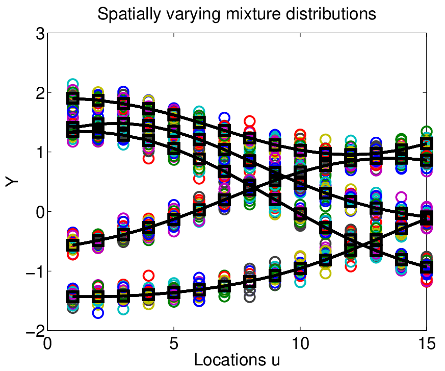
We generate two data sets of spatially varying clustered populations (see Fig. 3 for illustrations). In both data sets, we set . For data set A, global factors are generated from a Gaussian process (GP). These global factors provide support for 15 spatially varying mixtures of normal distributions, each of which has 5 mixture components. The likelihood is given by . For each we generated independently 100 samples from the corresponding mixture (20 samples from each mixture components). Note that each circle in the figures denote a data sample. This kind of data can be encountered in tracking problems, where the samples associating with each covariate can be viewed as a snapshot of the locations of moving particles at time point . The particles move in clusters. They may switch clusters at any time, but the identification of each particle is not known as they move from one time step to the next. The clusters themselves move in relatively smoother paths. Moreover, the number of clusters is not known. It is of interest to estimate the cluster centers, as well as their moving paths. 33 3 Particle-specific tracking is possible if the identity of the specific particle is maintained across snapshots. For data set B, to illustrate the variation in the number of local clusters at different locations, we generate a number of global factors that simulate the bifurcation behavior in a collection of longitudinal trajectories. Here a trajectory corresponds to a global factor. Specifically, we set . Starting at there is one global factor, which is a random draw from a relatively smooth GP with mean function , where and the exponential covariance function parameterised by , . At , the global factor splits into two, with the second one also an independent draw from the same GP, which is re-centered so that its value at is the same as the value of the previous global factor at . At , the second global factor splits once more in the same manner. These three global factors provide support for the local clusters at each . The likelihood is given by a normal distribution with . At each we generated 30 independent observations.
Although it is possible to perform clustering analysis for data at each location , it is not clear how to link these clusters across the locations, especially given that the number of clusters might be different for different ’s. The nHDP mixture model provides a natural solution to this problem. It is fit for both data sets using essentially the same prior specifications. The concentration parameters are given by and . is taken to be a mean-0 GP using for data set A, and for data set B. The variance is endowed with prior . The results of posterior inference (via MCMC sampling) for both data sets are illustrated by Fig. 4 and Fig. 5. With both data sets, the number global clusters are estimated almost exactly (5 and 3, respectively, with probability ). The evolution of the posterior distributions on the number of local clusters for data set B is given in Fig. 7. In both data sets, the local factors are accurately estimated (see Figs. 4 and 5). For data set B, due to the varying number of local clusters, there are regions for , specifically the interval where multiple global factors alternate the role of supporting local clusters, resulting in wider credible bands.
In Section 3 we discussed the implications of prior specifications of the base measure for the identifiability of global factors. We have performed a sensitivity analysis for data set A, and found that the inference for global factors is robust when is set to be in . For , for instance, which implies that are weakly dependent across ’s, we are not able to identify the desired global factors (see Fig. 6), despite the fact that local factors are still estimated reasonably well.
The effects of prior specification for on the inference of global factors are somewhat similar to the hybrid DP model: a smaller encourages higher numbers of and less smooth global curves to expand the coverage of the function space (see Sec. 7.3 of Nguyen and Gelfand (2010)). Within our context, the prior for is relatively more robust than that of as discussed above. The prior for concentration parameter is extremely robust while the priors for ’s are somewhat less. We believe the reason for this robustness is due to the modeling of the global factors in the second stage of the nested hierarchy of DPs, and the inference about these factors has the effect of pooling data from across the groups in the first stage. In practice, we take all ’s to be equal to increase the robustness of the associated prior.
Progesterone hormone clustering.
We turn to a clustering analysis of Progesterone hormone data. This data set records the natural logarithm of the progesterone metabolite, measured by urinary hormone assay, during a monthly cycle for 51 female subjects. Each cycle ranges from -8 to 15 (8 days pre-ovulation to 15 days post-ovulation). We are interested in clustering the hormone levels per day, and assessing the evolution over time. We are also interested in global clusters, i.e., identifying global hormone pattern for the entire monthly cycle and analyzing the effects on contraception on the clustering patterns. See Fig. 8 for the illustration and Brumback and Rice (1998) for more details on the data set.
For prior specifications, we set , and for all . Let . For , we set , and . It is found that the there are 2 global clusters with probability close to 1. In addition, the mean estimate of global clusters match very well with the sample means from the two groups of women, a group of those using contraceptives and a group that do not (see Fig. 9). Examining the variations of local clusters, there is a significant probability of having only one local cluster during the first 20 days. Between day 21 and 24 the number of local clusters is 2 with probability close to 1.
To elaborate the effects of contraception on the hormone behavior (the last 17 female subjects are known to use contraception), a pairwise comparison analysis is performed. For every two hormone curves, we estimate the posterior probability that they share the same local cluster on a given day, which is then averaged over days in a given interval. It is found that the hormone levels among these women are almost indistinguishable in the first 20 days (with the clustering-sharing probabilities in the range of ), but in the last 4 days, they are sharply separated into two distinct regimes (with the clustering- sharing probability between the two groups are dropped to ).
We compare our approach to the hybrid Dirichlet process (hybrid-DP) approach (Petrone et al., 2009; Nguyen and Gelfand, 2010), perhaps the only existing approach in the literature for joint modeling of global and local clusters. The data are given to the hybrid-DP as the replicates of a random functional curve, whereas in our approach, such functional identity information is not used. In other words, for us only a collection of hormone levels across different time points are given (i.e., the subject ID of hormone levels are neither revealed nor matched with one another across time points). For a sensible comparison, the same prior specification for base measure of the global clusters were used for both approaches. The inference results are illustrated in Fig. 9. A close look reveals that the global clusters obtained by the hybrid-DP approach is less faithful to the contraceptive/no contraceptive grouping than ours. This can be explained by the fact that hybrid-DP is a more complex model that directly specifies the local cluster switching behavior for functional curves. It is observed in this example that an individual hormone curve tends to over-switch the local cluster assignments for , resulting in significantly less contrasts between the two group of women (see Fig. 10 and 12). This is probably due the complexity of the hybrid-DP, which can only be overcome with more data (see Propositions 7 and 8 of Nguyen and Gelfand (2010) for a theoretical analysis of this model’s complexity and posterior consistency). Finally, it is also worth noting that the hybrid-DP approach practically requires the number of clusters to be specified a priori (as in the so-called -hybrid-DP in Petrone et al. (2009)), while such information is directly infered from data using the nHDP mixture.
6 Discussions
We have described a nonparametric approach to the inference of global clusters from locally distributed data. We proposed a nonparametric Bayesian solution to this problem, by introducing the nested Hierarchical Dirichlet process mixture model. This model has the virtue of simultaneous modeling of both local clusters and global clusters present in the data. The global clusters are supported by a Dirichlet process, using a stochastic process as its base measure (centering distribution). The local clusters are supported by the global clusters. Moreover, the local clusters are randomly selected using another hierarchy of Dirichlet processes. As a result, we obtain a collection of local clusters which are spatially varying, whose spatial dependency is regulated by an underlying spatial or a graphical model. The canonical aspects of the nHDP (because of its use of the Dirichlet processes) suggest straightforward extensions to accomodate richer behaviors using Poisson-Dirichlet processes (also known as the Pittman-Yor processes), where they have been found to be particularly suitable for certain applications, and where our analysis and inference methods can be easily adapted. It would also be interesting to consider a multivariate version of the nHDP model. Finally, the manner in which global and local clusters are combined in the nHDP mixture model is suggestive of ways of direct and simultaneous global and local clustering for various structured data types.
7 Appendix
7.1 Marginal approach to sampling
The Pólya-urn characterization suggests a Gibbs sampling algorithm to obtain posterior distributions of the local factors ’s and the global factors ’s, by integrating out random measures and ’s. Rather than dealing with the ’s and directly, we shall sample index variables and instead, because ’s and ’s can be reconstructed from the index variables and the ’s. This representation is generally thought to make the MCMC sampling more efficient. Thus, we construct a Markov chain on the space of . Although the number of variables is in principle unbounded, only finitely many are actually associated to data and represented explicitly.
A quantity that plays an important role in the computation of conditional probabilities in this approach is the conditional density of a selected collection of data items, given the remaining data. For a single observation -th at location , define the conditional probability of under a mixture component , given and all data items except :
| (18) |
Similary, for a collection of observations of all data such that for a chosen , which we denote by vector , let be the conditional probability of under the mixture component , given and all data items except .
Sampling . Exploiting the exchangeability of the ’s within the group of observations indexed by , we treat as the last variable being sampled in the group. To obtain the conditional posterior for , we combine the conditional prior distribution for with the likelihood of generating data . Specifically, the prior probability that takes on a particular previously used value is proportional to , while the probability that it takes on a new value is proportional to . The likelihood due to given for some previously used is . Here, . The likelihood for is calculated by integrating out the possible values of :
| (19) |
where is the prior density of . As a result, the conditional distribution of takes the form
| (20) |
If the sampled value of is , we need to obtain a sample of by sampling from Eq. (19):
| (21) |
Sampling . As with the local factors within each group, the global factors ’s are also exchangeable. Thus we can treat for a chosen as the last variable sampled in the collection of global factors. Note that changing index variable actually changes the mixture component membership for relevant data items (across all groups ) that are associated with , the likelihood obtained by setting is given by , where denotes the vector of all data such that . So, the conditional probability for is:
| (22) |
where .
Sampling of and . We follow the method of auxiliary variables developed by Escobar and West (1995) and Teh et al. (2006). Endow with a prior. At each sampling step, we draw . Then the posterior of is can be obtained as a gamma mixture, which can be expressed as , where . The procedure is the same for each , with and playing the role of and , respectively. Alternatively, one can force all to be equal and endow it with a gamma prior, as in Teh et al. (2006).
References
- Aldous (1985) Aldous, D. (1985), “Exchangeability and related topics,” École d’Été de Probabilités de Saint-Flour XIII-1983, 1–198.
- Antoniak (1974) Antoniak, C. (1974), “Mixtures of Dirichlet Processes with Applications to Bayesian Nonparametric Problems,” Annals of Statistics, 2, 1152––1174.
- Blackwell and MacQueen (1973) Blackwell, D. and MacQueen, J. (1973), “Ferguson Distributions via Polya Urn Schemes,” Annals of Statistics, 1, 353–355.
- Brumback and Rice (1998) Brumback, B. and Rice, J. (1998), “Smoothing spline models for the analysis of nested and crossed samples of curves,” J. Amer. Statist. Assoc., 93, 961–980.
- Cifarelli and Regazzini (1978) Cifarelli, D. and Regazzini, E. (1978), “Nonparametric statistical problems under partial exchangeability: The role of associative means,” Tech. rep., Quaderni Istituto Matematica Finanziaria dell’Universit‘a di Torino.
- Cressie (1993) Cressie, N. (1993), Statistics for Spatial Data, Wiley, NY.
- DeIorio et al. (2004) DeIorio, M., Mueller, P., Rosner, G., and MacEachern, S. (2004), “An ANOVA model for dependent random measures,” J. Amer. Statist. Assoc., 99, 205–215.
- Duan et al. (2007) Duan, J., Guindani, M., and Gelfand, A. (2007), “Generalized spatial Dirichlet processes,” Biometrika, 94, 809–825.
- Dunson (2008) Dunson, D. (2008), “Kernel local partition processes for functional data,” Tech. Rep. 26, Department of Statistical Science, Duke University.
- Dunson and Park (2008) Dunson, D. and Park, J.-H. (2008), “Kernel stick-breaking processes,” Biometrika, 95, 307–323.
- Escobar and West (1995) Escobar, M. and West, M. (1995), “Bayesian Density Estimation and Inference Using Mixtures,” Journal of the American Statistical Association, 90, 577––588.
- Ferguson (1973) Ferguson, T. (1973), “A Bayesian analysis of some nonparametric problems,” Ann. Statist., 1, 209–230.
- Gelfand et al. (2005) Gelfand, A., Kottas, A., and MacEachern, S. (2005), “Bayesian nonparametric spatial modeling with Dirichlet process mixing,” J. Amer. Statist. Assoc., 100, 1021–1035.
- Griffin and Steel (2006) Griffin, J. and Steel, M. (2006), “Order-based dependent Dirichlet processes,” J. Amer. Statist. Assoc., 101, 179–194.
- Hjort et al. (2010) Hjort, N., Holmes, C., Mueller, P., and (Eds.), S. W. (2010), Bayesian Nonparametrics: Principles and Practice, Cambridge University Press.
- Ishwaran and James (2001) Ishwaran, H. and James, L. (2001), “Gibbs sampling methods for stick-breaking priors,” J. Amer. Statist. Assoc., 96, 161–173.
- Ishwaran and Zarepour (2002a) Ishwaran, H. and Zarepour, M. (2002a), “Dirichlet prior sieves in finite normal mixtures,” Statistica Sinica, 12, 941–963.
- Ishwaran and Zarepour (2002b) — (2002b), “Exact and Approximate Sum-Representations for the Dirichlet Process,” Canadian Journal of Statistics, 30, 269––283.
- Jordan (2004) Jordan, M. (2004), “Graphical models,” Statistical Science, Special Issue on Bayesian Statistics (19), 140–155.
- Lauritzen (1996) Lauritzen, S. (1996), Graphical models, Oxford University Press.
- Lo (1984) Lo, A. (1984), “On a class of Bayesian nonparametric estimates I: Density estimates,” Annals of Statistics, 12, 351–357.
- MacEachern (1999) MacEachern, S. (1999), “Dependent Nonparametric Processes,” in Proceedings of the Section on Bayesian Statistical Science, American Statistical Association.
- MacEachern and Mueller (1998) MacEachern, S. and Mueller, P. (1998), “Estimating Mixture of Dirichlet Process Models,” Journal of Computational and Graphical Statistics, 7, 223––238.
- Mueller et al. (2004) Mueller, P., Quintana, F., and Rosner, G. (2004), “A Method for Combining Inference Across Related Nonparametric Bayesian Models,” Journal of the Royal Statistical Society, 66, 735–749.
- Muliere and Petrone (1993) Muliere, P. and Petrone, S. (1993), “A Bayesian Predictive Approach to Sequential Search for an Optimal Dose: Parametric and Nonparametric Models,” Journal of the Italian Statistical Society, 2, 349–364.
- Muliere and Secchi (1995) Muliere, P. and Secchi, P. (1995), “A note on a proper Bayesian bootstrap,” Tech. Rep. 18, Dipartimento di Economia Politica e Metodi Quantitativi, Universita degli Sudi di Pavia.
- Neal (1992) Neal, R. (1992), “Bayesian Mixture Modeling,” in Proceedings of the Workshop on Maximum Entropy and Bayesian Methods of Statistical Analysis, vol. 11, pp. 197––211.
- Nguyen and Gelfand (2010) Nguyen, X. and Gelfand, A. (2010), “The Dirichlet labeling process for clustering functional data,” Statistica Sinica, to appear.
- Petrone et al. (2009) Petrone, S., Guidani, M., and Gelfand, A. (2009), “Hybrid Dirichlet processes for functional data,” Journal of the Royal Statistical Society B, 71(4), 755–782.
- Pittman (2002) Pittman, J. (2002), “Poisson-Dirichlet and GEM invariant distributions for split-and-merge transformations of an interval partition,” Combinatorics, Probability and Computing, 11, 501–514.
- Rabiner (1989) Rabiner, L. (1989), “A Tutorial on Hidden Markov Models and Selected Applications in Speech Recognition,” Proceedings of the IEEE, 77, 257––285.
- Rodriguez and Dunson (2009) Rodriguez, A. and Dunson, D. (2009), “Nonparametric Bayesian models through probit stick-breaking processes,” Tech. rep., University of California, Santa Cruz.
- Rodriguez et al. (2010) Rodriguez, A., Dunson, D., and Gelfand, A. (2010), “Latent stick-breaking processes,” J. Amer. Statist. Assoc., 105(490), 647–659.
- Schwartz (1965) Schwartz, L. (1965), “On Bayes procedures,” Z. Wahr. Verw. Gebiete, 4, 10–26.
- Sethuraman (1994) Sethuraman, J. (1994), “A constructive definition of Dirichlet priors,” Statistica Sinica, 4, 639–650.
- Teh et al. (2006) Teh, Y., Jordan, M., Beal, M., and Blei, D. (2006), “Hierarchical Dirichlet processes,” J. Amer. Statist. Assoc., 101, 1566–1581.
- Teh and Jordan (2010) Teh, Y. W. and Jordan, M. I. (2010), “Hierarchical Bayesian nonparametric models with applications,” Bayesian Nonparametrics: Principles and Practice, In N. Hjort, C. Holmes, P. Mueller, and S. Walker (Eds.).
- Wainwright and Jordan (2008) Wainwright, M. J. and Jordan, M. I. (2008), “Graphical models, exponential families, and variational inference,” Foundations and Trends in Machine Learning, 1, 1–305.