New analytical progress in the theory of vesicles under linear flow
Abstract
Vesicles are becoming a quite popular model for the study of red blood cells (RBCs). This is a free boundary problem which is rather difficult to handle theoretically. Quantitative computational approaches constitute also a challenge. In addition, with numerical studies, it is not easy to scan within a reasonable time the whole parameter space. Therefore, having quantitative analytical results is an essential advance that provides deeper understanding of observed features and can be used to accompany and possibly guide further numerical development. In this paper shape evolution equations for a vesicle in a shear flow are derived analytically with precision being cubic (which is quadratic in previous theories) with regard to the deformation of the vesicle relative to a spherical shape. The phase diagram distinguishing regions of parameters where different types of motion (tank-treading, tumbling and vacillating-breathing) are manifested is presented. This theory reveals unsuspected features: including higher order terms and harmonics (even if they are not directly excited by the shear flow) is necessary, whatever the shape is close to a sphere. Not only does this theory cure a quite large quantitative discrepancy between previous theories and recent experiments and numerical studies, but also it reveals a new phenomenon: the VB mode band in parameter space, which is believed to saturate after a moderate shear rate, exhibits a striking widening beyond a critical shear rate. The widening results from excitation of fourth order harmonic. The obtained phase diagram is in a remarkably good agreement with recent three dimensional numerical simulations based on the boundary integral formulation. Comparison of our results with experiments is systematically made.
pacs
87.16.D- 83.50.Ha 87.17.Jj 83.80.Lz 87.19.rhI Introduction
A vesicle is a closed simply connected membrane separating two liquids. Its dynamics in an ambient flow is an important research target due to various medical applications. For instance, they are employed as biochemical reactors [1, 2], as vectors for targeted drug and gene delivery [3, 4], and as artificial cells for hemoglobin encapsulation and oxygen transport [5].
One can also regard a vesicle, from mechanical point of view, as a simplified model of a living cell. The most prominent biological counterpart for a vesicle is the red blood cell (RBC). The vesicle system allows to identify the elementary processes of visco-elastic properties of cells moving passively in a fluid. The study of a single vesicle under a shear flow is one of the simplest nonequilibrium example. Nevertheless, this problem gives rise to a very complicated dynamics with different types of vesicle motion because of the nontrivial competition between the interactions of straining and rotational parts of shear flow with the vesicle. Three main types of motion for a vesicle in a shear flow have been identified so far: (i) tank-treading (TT), when shape and orientation of the vesicle is a steady-state, (ii) tumbling (TB), when the vesicle makes full rotations, and (iii) vacillating-breathing (VB, aka trembling or swinging), when the longest axis of the vesicle oscillates around certain direction with the shape strongly changing during these oscillation cycles. Since many properties of a vesicle (e.g. the effective viscosity) strongly depend on its type of motion, it is important to define the phase diagram of a vesicle in a shear flow, predicting which type of motion will be realized for each set of parameters defining the vesicle dynamics.
A widely accepted model for a vesicle proposes the following assumptions: zero Reynolds number limit, membrane impermeability and local inextensibility, and the continuity of velocity field and mechanical stress across the membrane. The force exerted on the membrane by the liquids is balanced by the membrane rigidity force that is calculated from the energy of membrane bending taken as[6]
| (1) |
where is the bending rigidity coefficient of the membrane, is the mean curvature and is a Lagrange multiplier, ensuring the local membrane inextensibility. Under these assumptions, and after a certain choice of units for all variables, the vesicle dynamics can be completely described by three dimensionless numbers (see for example [7]): the viscosity contrast
| (2) |
the excess area relative to a sphere
| (3) |
and the capillary number
| (4) |
Here are the viscosities of fluids inside and outside the membrane respectively, is the surface area of the vesicle, is the radius of a sphere containing the same volume as the vesicle, and is the shear rate. It is convenient to choose as the unit of distance so that the volume of the vesicle is
| (5) |
We also use as the unit of viscosity and as the unit of time.
Several studies have been recently dedicated to the determination of the phase diagram regarding different types of motion of an almost spherical vesicle in a shear flow. These studies were theoretical[8, 9, 10, 11], experimental [12, 13, 14, 15], and numerical [17, 16]. Those theoretical works treat the membrane deviation from a spherical shape as a perturbation ( is the small expansion parameter), represented as a series of spherical harmonics. Then it is suggested that one or two first orders in the expansion of the shape evolution equations must be retained. Generally, the resulting equations differ only because the authors propose distinct rules of neglection. The Leading Order Theory[8] (LOT) keeps only the terms of order of the imposed flow and the effects of the vorticity in the final equations. This theory is precise up to in the expansion scheme. Later studies have included higher order terms in the expansion (up to . Lebedev et al. [11] included the next order terms in the membrane Helfrich force (as compared to LOT), while another study (hereafter called Higher Order Theory[10] (HOT)) accounted for the next order terms not only in the Helfrich force but also in the hydrodynamic field as well.
In the theories of Ref. [10] and Ref. [11], as well as in numerical studies based on dissipative particles dynamics [17], a saturation of the VB/TB phase border for large enough was suggested– i.e. the value of at which the transition from VB to tumbling occurs becomes almost independent on the capillary number (or equivalently on shear rate).
Recent advances in three dimensional numerical computations based on the boundary integral formulation [16] have made it possible to study vesicle dynamics quantitatively. The results of this study show, that the loss of stability of the TT solution occurs at values of significantly higher than those predicted by analytical calculations[10, 11]. Furthermore, no saturation of the VB/TB phase border upon increasing shear rate (or ) was found. These results provide a new input that is worth understanding from the analytical point view.
The main objective of this work is to investigate the reasons for the discrepancies between the results provided by the recent numerical simulations [16] and analytical theories. It was pointed out in Ref.[11] that the critical values of at which the steady-state solution loses its stability, scales as for a fixed shear rate. However, this behaviour, which also agrees with the result of Keller and Skalak [18], does not provide the correct information about the next order terms, as will be seen here. The next correction turns out to cause a rather big shift of the phase borders.
This peculiar behavior (i.e. that the critical diverges at vanishing ) confers to the vesicle problem a special status: in the small limit, one further order and only one in the expansion scheme in powers of is needed as compared to previous studies. As a consequence, it will be shown, in particular, that the next order term, previously unaccounted for, survives whatever small the deviation from a sphere is. This is the source of deviation between the recent numerical work and the existing analytical theories. As will be seen inclusion of one more order in the expansion will allow us to extract a phase diagram that is in quantitative agreement with the results of numerical simulations[16]. It will also be shown that fourth order spherical harmonics (in previous theories only second order harmonics were included) can not be neglected, and especially beyond a certain shear rate. Indeed, it will be revealed that these harmonics give rise to a new important feature recently revealed in numerical simulations [16]. More precisely, the VB/TB phase border does not saturate for fixed when shear rate exceeds a certain value, rather a significant widening is revealed, in contrast to previous theoretical [11, 10], numerical [17] and experimental investigations [14].
II Shape evolution equations
II.1 Basic definitions and the expansion scheme
Here we perform the expansion of the shape evolution equations one order higher as compared to the most advanced of previous papers[10]. Since a slightly deflated vesicle in the absence of flow takes a centro-symmetric shape, and the shear flow has a symmetry center in every point, we consider only symmetric shapes.
Naturally, we take the origin of coordinates at the center of the vesicle moving with the velocity of the undisturbed shear flow. That the vesicle moves with the same velocity as the applied shear flow is a consequence of the symmetry of the problem. We use the conventional parametrization of the vesicle membrane with reference points belonging to a sphere of radius unity
| (6) |
The shape function is then expanded in spherical harmonics of Note that the shape depends also on time, but the temporal variable will be specified only when need be. Following Ref.[9, 10] we introduce a formal expansion parameter which helps classifying different orders. Only second order harmonics are present to the order of in the equilibrium shape function of an almost spherical vesicle in the absence of flow. They are also the only harmonics that can interact with linear flow directly. For consistency considerations, pushing the expansion to next order implies that the fourth and zeroth order harmonics cannot be neglected. They enter dynamics as a result of interactions between the vesicle shape and the Helfrich force and the flow; they are of order The shape function does not contain spherical harmonics of odd orders owing to the centro-symmetry. The spherical harmonics of even orders higher than have an amplitude and thus are neglected. As follows from the inequality
the average radius of the vesicle is not exactly 1. Therefore a negative correction must be added to it in order to satisfy (5). This correction is of order and leads to a non-zero coefficient for zero-order spherical harmonic in the expansion of which will be denoted below.
The expansion takes formally the form:
| (7) |
There are various definitions of spherical harmonics, here we use those that satisfy the following normalization conditions:
However, all equations are written in universal form and are valid for any rescaling of spherical harmonics.
The condition (5) together with the definition provide two additional constraints on the coefficients of the expansion (7). We use the former to express through
| (8) |
and the latter to norm the coefficients
| (9) |
We retain one more order in these expressions compared to previous works for the sake of consistency. Note that the volume and the surface have been expanded to the order in order to obtain the equalities (8) and (9).
II.2 Derivation of the evolution equations of the from the boundary integral formulation
We shall adopt here a different spirit from that of previous theories [8, 10, 11, 9]. There the Lamb solution is used (a solution of the Stokes equations inside and outside the vesicle). We find it convenient to take the boundary integral formulation as a starting point. The present spirit is equivalent to using the Lamb solution, but it has the advantage that the boundary conditions at the membrane are already implemented in the boundary integral formulation. Indeed, the Stokes equations together with the boundary conditions on the membrane, and far away from it, can be converted into boundary integral formulation [19]. This leads to the following integral equation
| (10) |
Here is the actual velocity of point is the velocity of point in the imposed flow, is the membrane rigidity force at point is the outward pointing normal to the vesicle surface at point The integration is taken over the surface of the vesicle and is the surface area element. The integration kernels have the following form:
Using the expression for the Helfrich force, we can find from (10) the velocity field on the surface of the vesicle. The Helfrich force is given in terms of the shape as
| (11) |
where is the Gaussian curvature and is the Laplace-Beltrami operator. It can easily be checked that expression (11) vanishes for a spherical shape, and thus is of order In order to balance (10) at order we need to assume the imposed flow to be of the same order as (11). This requirement can equivalently be fulfilled, following Refs. [8, 10], by the demand that scale as We then set with of order
The precise technical details will be given elsewhere, while here we shall present only the spirit and some intermediate steps. We expand and into vector spherical harmonics of For convenience we define them as
Here the differentiation with respect to is taken formally as if were a regular 3D vector not bound to a sphere of radius unity, and is the Levi-Civita (unit anti-symmetric) tensor. The advantage of such a definition is that not only do these spherical harmonics constitute an orthogonal set with respect to the integration of dot product over i.e. the quantity
is zero unless but also operators and are diagonal in the chosen basis for a spherical vesicle, so that the integrals
are zero unless Given the centro-symmetry we impose, in our expansion of and the absence of for even and and for odd In order to find the evolution equations we need to expand the velocity field to the order of Coefficients for for are and thus can be neglected. It will be shown later that coefficients of 5th and 6th orders of vector spherical harmonics make corrections to the evolution equations for with which are So only five first orders (starting from the zeroth one) of vector spherical harmonics should be taken into account in the expansion of any space-dependent quantity under consideration.
In order to fulfil the condition of local inextensibility of the membrane we impose zero surface divergence of the velocity field[8].
| (12) |
Here
is the Jacobian matrix. We can take the derivatives as if were a regular 3D vector, because the surface divergence is fully determined by the distribution of the velocity field on the membrane and does not depend on the continuation of the flow into the liquids.
We expand equations (10,12) to order and the resulting integrals could be performed analytically. Projecting the results of the integration on the space of vector spherical harmonics up to the fourth order, we obtain a set of equations satisfied by the coefficients entering the expansions of and Since the surface area is evaluated up to order while the velocity field in (12) is expanded only up to order it is not appropriate to use (12) in order to ensure the conservation of the whole surface area. Therefore, we only use the projections of (12) on for equal to or Accordingly, we leave the isotropic part of (denoted here as ) undetermined. Once the final shape evolution equations are obtained we shall use the constraint that the time derivative of (9) is equal to zero in order to determine This way of reasoning was used in previous studies [8, 10, 9, 11]. Note that unlike other theories [8, 10, 9, 11], since we expand the equations to higher order, it is not legitimate to replace in (12) with prior to projection on the spherical harmonics sub-space. Such a substitution would imply neglecting terms of order in final equations, and would be inconsistent with the spirit of the present theory.
Having determined the velocity field thanks to the above expansions, we are in a position to obtain the final evolution equation by making use of the kinematic equation expressing the fact that the membrane velocity is equal to the fluid velocity at the membrane
| (13) |
Then the task is to substitute the expanded velocity field into this equation (in terms of coefficients of the velocity field) and project the resulting expression onto the space of spherical harmonics of interest. This then leads to the determination of the evolution equations that must be satisfied by the shape coefficients It can be shown that the following identities hold and Therefore the projection of the first part of the right hand side of (13) on the subspace of spherical harmonics of orders up to four does not depend on the coefficients of the vector spherical harmonics of orders five and six in the velocity field. Regarding the the second part, is of order and the coefficients for fifth and sixth orders of vector spherical harmonics in the velocity field expansion are of order so that their contribution in the shape evolution equation is of order that is beyond our accuracy.
It is convenient to decompose the applied shear flow into its elongational and rotational parts to simplify the final equations. The same decomposition can be applied to general linear flow: the quantity defines the straining part, while the vector represents the vorticity. Note, that in (10) is the velocity of the imposed flow evaluated at the point which takes the following form
The shape evolution equations for the second and fourth order harmonics can be written in a compact form:
| (14) |
| (15) |
The left hand side term of the equation is a special derivative of that naturally arises in a non-rotating coordinate system, and its definition is
| (16) |
To the order at which our expansion is performed, the rotational velocity of the vesicle is not equal to the vorticity of the imposed flow (unlike lower order calculations [8, 9, 10, 11]), but rather it has a new contribution originating from the shape function
| (17) |
Note that if only the first term is retained [8, 9, 10, 11], then (16) coincides with the Jaumann derivative.
The functions can be written as
The coefficients and are rational functions of and The exact expressions are listed in the appendix.
III The phase diagram
III.1 The analytical phase diagram and comparison with previous works

The phase diagram for is presented on the Fig.1. The value is chosen for the sake of comparison with available numerical data [16]. Also shown on that Figure are the results obtained in two previous theories[10, 11]. As can be seen the basic structure of the phase diagram bears similarity with previous ones. There are however some important distinctions. First, the phase borders are significantly shifted towards the region of higher viscosity contrasts. Second, the VB/TB transition curve does not saturate upon increasing shear rate (or ), rather it exhibits a striking widening. We have also compared the results with those obtained recently by full three dimensional simulations. A remarkable agreement between the two approaches is found (see comparison in Ref. [16]).
III.2 Basic reasons for necessity of higher order expansion
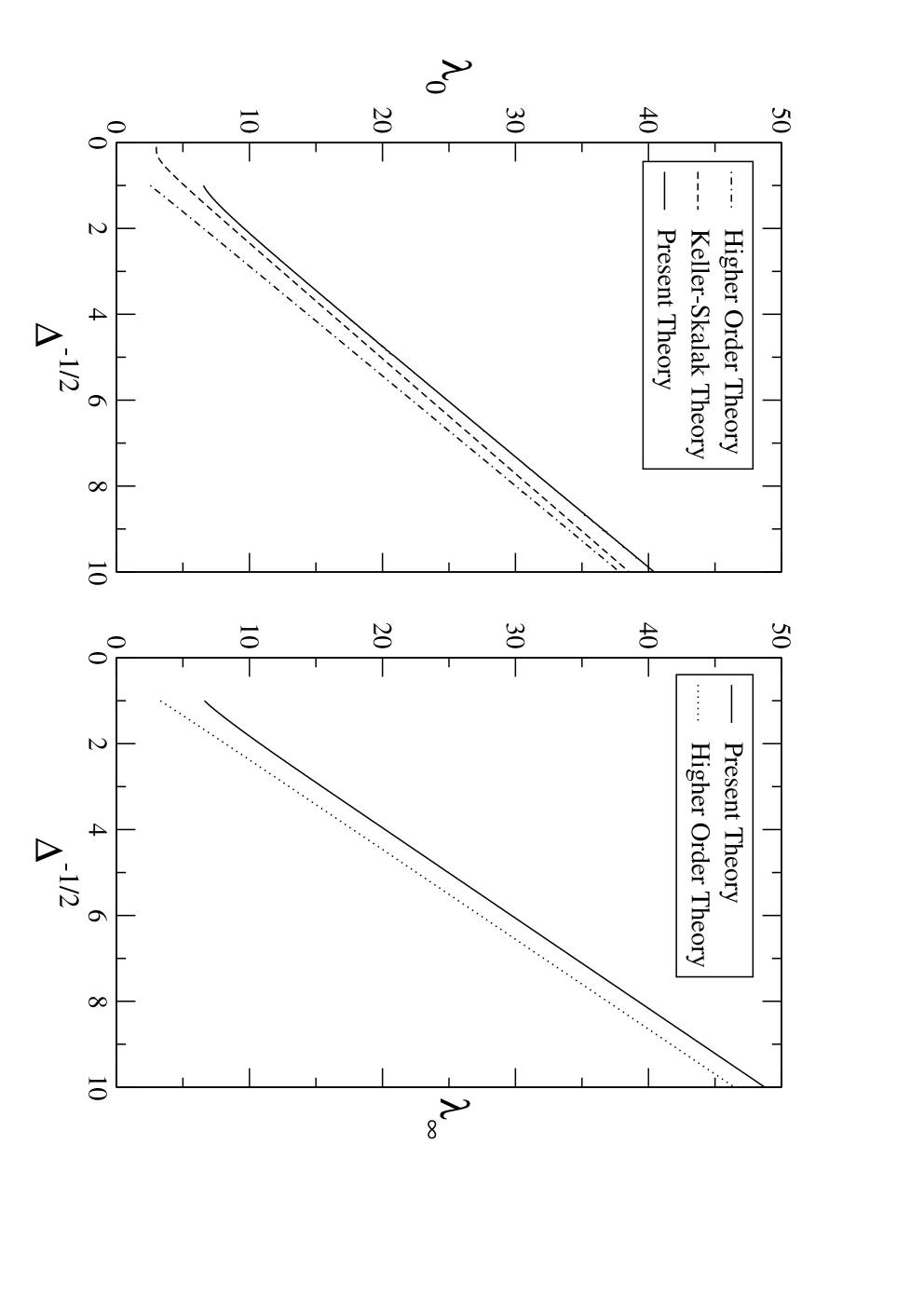
Our first concern is to understand why the inclusion of the terms of order provides such a dramatic shift of the phase borders even though the shape is almost spherical (the relative excess area is only ). We have studied the evolution of the phase diagram as a function of in order to gain further insight. We have tracked the viscosity contrast at which the loss of stability of TT motion occurs in the two asymptotic limits (the corresponding value is denoted as ) and (denoted as ). It was reported in [11] that Since we expect the expansions of to be analytic in we have thus attempted the following ansatz:
| (18) |
To check the validity of this expansion we plot these critical values as a function of We expect then a linear behavior. This is presented on Fig.2 where we also compare our results with those of previous theories. A key point to be discussed further below is the fact that previous theories provide correct values for the dominant term in the expansions (18), but not for which does not vanish even in the limit of almost spherical vesicles (note that the next order terms in the expansion (18) tend to with the excess area). Because remains finite whatever small is the deviation from a sphere, the discrepancy between the TT phase borders obtained by different theories (with one lower order below the present one, namely of the order of ) persists for any excess area. In contrast the present theory valid to order has the property that even if one wishes to make an expansion to the next order (i.e. order ), then the shift in the borders in the phase diagram would be negligibly small, i.e. the shift would vanish in the small excess area limit. In other words, the present theory shows that there is a convergence of the small deformation scheme at order This implies that there is no need to continue the expansion of the shape evolution equation beyond the order since this would neither notably modify the results for nor significantly extend the applicability to higher values of Comparison of the present theory with numerical results (see comparison provided in Ref. [16]) shows a good agreement for (the only value explored to date by the numerical scheme).
III.3 Discussion of the tank-treading phase borders
As can be seen the dependencies shown on Fig.2 are fairly linear for and are almost indistinguishable from straight lines for The region of where the curves noticeably deviate from straight lines is wider for present theory than for HOT. This is most likely caused by the introduction of fourth order spherical harmonics, their amplitude is no more small compared to that of the second order harmonics for The expression (9) becomes inapplicable, and as a result grow uncontrollably with time in solutions of the differential equations. This problem can be fixed by expanding the excess area to the order but the results of such patching are not trustworthy because they go beyond the precision of the differential equations.
Note also that the second term in (17) tends to align the vesicle to the elongating direction of the straining part of the shear flow which makes the angle with the direction of the flow. In the TT phase close to the loss of the stability of the steady-state solution the vesicle is almost parallel to the flow. The effective vorticity (17) turns out to be less than in the TT phase, and it leads to the increased stability of the steady-state solution. The correction to the vorticity is proportional to and thus increases with and dominates over in the large excess area limit. As a consequence, the truncation (17) becomes illegitimate. Generally, we may assert that is a good estimate for the applicability limits of the small deformation approximation.
Some theories[8, 11, 18] allow for analytical extraction of the coefficients and and for HOT and the present theory the extraction is numerical by using the slope and offset of the lines on the Fig.2. The combined data are presented in the tables 1 and 2.
| Theory | ||
|---|---|---|
| LOT[8] | ||
| HOT[10] | ||
| Lebedev et al.[11] | ||
| Keller and Skalak [18] | ||
| Present | 3.89 | 1.54 |
| Theory | ||
|---|---|---|
| LOT[8] | ||
| HOT[10] | ||
| Lebedev et al.[11] | ||
| Present | 4.76 | 1.13 |
HOT and Lebedev et al. theories show a good agreement for the coefficients with the present calculation. This means, that expansion of the shape evolution equations to the order was indeed sufficient in order to capture the correct value of even for large values of where Lebedev et al. theory loses its applicability. The present theory shows that the correct value of is captured thanks to the fact that the expansion scheme is pushed one step further in the excess area. Keller-Skalak theory gives a slightly different result for the difference is caused by the fact they used a velocity field having a surface divergence of order whereas the membrane local inextensibility requires zero surface divergence instead. On the other hand Keller-Skalak theory provides a better estimate for the value of than the one proposed by HOT and this explains why its results are relatively close to the results of numerical simulations for
III.4 Discussion of TB/VB transition
We plan to dedicate a separate research to the properties of different types of vesicle motion, so here we only briefly discuss further implication of the new theory on the TB/VB transition. Neglecting harmonics of orders higher than two, as done in previous theories, provides two major simplifications. First, the vesicle shape has three symmetry planes, which make the definition of the orientation angle obvious, and second the in-plane motion is defined by only two independent variables. As a consequence, the dynamics relaxes with time to a cyclic motion (which degenerates into a point in the TT phase). Thus only a simple limit cycle can exist, and this shows that each of the VB and TB modes has its own region of existence in parameter space. The above assertions can not be made in general, and especially when the fourth order harmonics are included. It also turns out that near the transition region the vesicle tends to finish its TB quasi-cycles by assuming an oblate almost axisymmetric shape in the shear plane rather than an elongated shape perpendicular to the flow. For such shape the error in the definition of the orientation angle is very large.
Let us now discuss how each type of motion is determined from our evolution equations. We start with some initial values for and wait a ceratin time interval until the initial data are irrelevant. Then it was checked whether during one oscillation quasi-cycle has a maximum for lying in the shear plane and perpendicular to the shear velocity. Despite some noise due to the aforementioned complications it is clearly seen that unlike with previous theories the VB/TB phase border does not saturate even for and the VB region broadens with the increase of the capillary number (Fig. 1).
Note that it was suggested recently [20] that higher orders of spherical harmonics can be excited close to the VB/TB phase border and this may cause some widening of the VB phase region (but still saturation at large is found, unlike our theory). It can be checked that when , the fourth order harmonics are excited (i.e. the corresponding decay time becomes infinite to leading order). Here, we found that close to the VB/TB transition at some times during the oscillation the quantity
| (19) |
exceeds 20. This is probably the reason why the VB/TB phase border remains unsaturated for much larger values than in previous analytical studies. It was proposed in [20], however, that excitation of higher harmonics was due to thermal fluctuations. This contrasts in spirit with our theory where the fourth order harmonic is excited as non-linear interaction of second harmonics and no reference to temperature is required.
IV Comparison with experiments
Experiments have been performed recently regarding determination of the phase diagram of vesicle motions under shear flow[14]. They referred to a previous theoretical work [11] which had suggested that the phase diagram should depend on only two independent dimensionless control parameters (and not three), namely
| (20) |
It has been reported [14] (with a certain degree of uncertainty) that the experimental data were consistent with the fact that only the above two parameters determine the phase diagram. Our results do not comply with this report, as shown on Figure 3. Indeed, besides and , the excess area plays an important role. Experiments mixed data for different ’s in the plane . The band of the VB mode in experiments looks quite wide, and we believe that this reflects the sensitivity of the location of the VB band to excess area (in other words the experimental data may be viewed as juxtaposition of bands each representing a value of ; see the example of Figure 3). It is hoped that a study representing each value of will be performed in the future with the aim of making comparison with theory clearer.

Furthermore, it must be noted that our estimates for the TT-VB phase borders are higher than those observed in experiments. This is not very surprising since transients are found to be very long close to TT-VB transition (as also discussed in our recent full numerical simulations [16]), and therefore a firm conclusion on the type of motion can not be made on the basis of the current experimental data, which are limited to only few periods of oscillation (while transient can exhibit up to hundreds of cycles as discussed recently [16]). In other words, this kind of long relaxation would convey the impression that dynamics is of VB type, whereas in reality it is a TT one.


Other experiments[15] were performed under linear flow with applied velocity field , which is different from a simple shear flow. The experiments were performed with no viscosity contrast and the ratio of the rotational () and the straining () parts of the flow was varied instead. The results of the experiments were plotted in coordinates
| (21) |
representing the generalization of (20). It was then claimed [15] that the phase diagram depends on these two parameters only (at least with no viscosity contrast). The Fig.4 simulates this experiment using the present theory. The discrepancy between resulting phase diagrams for various values of is indeed not as striking as for the simple shear flow (Fig.3): the TT phase borders fall close to each other and VB bands overlap for a wide range of At the same time, the VB/TB phase borders still vary significantly with the excess area. However, by fixing and varying we can produce series of phases diagrams in the and plane corresponding to different values of (see Fig.5). Here we find the same kind of discrepancy as on Fig.3 .
Finally, let us compare our results with other set of experiments in the TT regime[13]. We represent the vesicle orientation angle under strong shear flow(Fig. 3) (for the sake of comparison with experiments which were performed at high shear rates). It can be checked that the exact form of the bending energy becomes insignificant under strong flows, because the dominant contribution to the membrane force comes form the tension part which enforces incompressibility of the membrane. Unlike for the VB/TB phase border, the dependence of on quickly saturates with We take in our calculation. We use the artificial parameter (20) instead of in order to show the effect of terms taken into account by the present calculation. Note that the results of Lebedev it et al. theory [11] do not depend on the excess area in this representation, unlike our results and those reported by experiments (see Fig. 5). The results of HOT depend also on , but that dependence is weak so that they hardly differ from theoretical results of Ref.[11] (we do not plot them here in order to avoid encumbering of the figure). Experimental results[13] are provided for four different values of and We exclude , since we do not expect our theory to be applicable to a such large value of excess area. As can be seen, theoretical results and experimental ones show a rather good agreement provided that one is not close to the TT/VB border (i.e. if the angle is not too close to zero). The discrepancy for small inclination angles may be attributed to thermal fluctuations or interactions with walls. However, a systematic theoretical study of these factors should be performed before drawing conclusive answers.

V Discussion and conclusion
Here we have presented a small deformation theory of a vesicle in shear flow keeping one more order in the expansion of the shape evolution equations than prior studies. We have confirmed the leading term in the asymptotic expansion of critical viscosity ratios determined by previous analytical studies, but we also were able to determine accurately the next term in the expansion. This term is constant and survives no matter how small the excess area is. Moreover, this theory provides a correction to the phase borders that is significant in a wide range of excess areas. Unlike previous analytical works, but in agreement with the results of the numerical simulations [16], we observe an unsaturated growth of the VB/TB phase border in a quite large range of the capillary number.
We hope that this work will incite future experimental research. It will also be interesting to investigate experimentally the presence of widening of the VB band as a function of shear rate. Finally, we did not include third order spherical harmonics in the expansion of the shape function, restricting our calculations only to centro-symmetric vesicles. In the full numerical simulation [16], no symmetry restriction is imposed and so far no manifestation of the third order harmonic has been observed. This confers to our assumption of centro-symmetry a certain legitimacy.
Acknowledgements: We would like to thank G. Danker, S. S. Vergeles, and P. M. Vlahovska for helpful discussions. A.F. and C.M. acknowledge financial support from CNES (Centre National D’études Spatiales) and ANR (Agence Nationale pour la Recherche); "MOSICOB project".
Appendix A The shape evolution equations and the expression of various coefficients in terms of physical parameters
We remind that
The coefficients are then written as
References
- [1] V. Noireaux, A. Libchaber, PNAS 101, 17669–17674 (2004).
- [2] M. Karlsson, M. Davidson, R. Karlsson, A. Karlsson, J. Bergenholtz, Z. Konkoli, A. Jesorka, T. Lobovkina, J. Hurtig, M. Voinova, O. Orwar, Ann. Rev. Phys. Chem. 55, 613–649 (2004).
- [3] T. M. Allen, P. R. Cullis, Science 303, 1818–1822 (2004).
- [4] G. Gregoriadis, Trends Biotechnol. 13, 527–537 (1995).
- [5] D. R. Arifin, A. F. Palmer, Biomacromolecules 6, 2172–2181 (2005).
- [6] W. Helfrich, Z. Naturforsch. 28c, 693-703 (1973).
- [7] B. Kaoui, A. Farutin, and C. Misbah, Phys. Rev. E. 80 061905 (2009).
- [8] C. Misbah. Phys. Rev. Lett 96, 028104 (2006).
- [9] P. M. Vlahovska, R. S. Gracia. Phys. Rev. E 75, 016313 (2007).
- [10] G. Danker, T. Biben, T. Podgorski, C. Verdier, C. Misbah, Phys. Rev. E 76, 041905 (2007).
- [11] V. V. Lebedev, K. S. Turitsyn, S. S. Vergeles, Phys. Rev. Lett. 99, 218101 (2007).
- [12] M. Mader, V. Vitkova, M. Abkarian, A. Viallat, T. Podgorski, Eur. Phys. J. E 19, 389 (2006).
- [13] V. Kantsler, V. Steinberg, Phys. Rev. Lett. 96, 036001 (2006).
- [14] J. Deschamps, V. Kantsler, V. Steinberg, Phys. Rev. Lett. 102, 118105 (2009).
- [15] J. Deschamps, V. Kantsler, E. Segre, V. Steinberg, PNAS 106 11444 (2009).
- [16] T. Biben, A. Farutin, C. Misbah, arXiv:0912.4702v1.
- [17] H. Noguchi, G. Gompper. Phys. Rev. Lett. 98, 128103 (2007).
- [18] S. R. Keller, R. Skalak, J. Fluid Mech. 120, 27 (1982).
- [19] C. Pozrikidis, Boundary integral and singularity methods for linearized viscous flow, Cambridge University Press (1992).
- [20] S. S. Vergeles, V. V. Lebedev, K. S. Turitsyn (unpublished) (2009).