Gravitational instability of the inner static region of a Reissner-Nordström black hole

Gustavo Dotti and Reinaldo J. Gleiser Affiliation: Facultad de Matemática, Astronomía y Física (FaMAF), Universidad Nacional de Córdoba and
Instituto de Física Enrique Gaviola, CONICET.
Ciudad Universitaria, (5000) Córdoba, Argentina

Abstract

Reissner–Nordström black holes have two static regions: $r>r_{o}$ and $0<r<r_{i}$ , where $r_{i}$ and $r_{o}$ are the inner and outer horizon radii. The stability of the exterior static region has been established long time ago. In this work we prove that the interior static region is unstable under linear gravitational perturbations, by showing that field perturbations compactly supported within this region will generically excite a mode that grows exponentially in time. This result gives an alternative reason to mass inflation to consider the space time extension beyond the Cauchy horizon as physically irrelevant, and thus provides support to the strong cosmic censorship conjecture, which is also backed by recent evidence of a linear gravitational instability in the interior region of Kerr black holes found by the authors. The use of intertwiners to solve for the evolution of initial data plays a key role, and adapts without change to the case of super-extremal Reissner-Nordström black holes, allowing to complete the proof of the linear instability of this naked singularity. A particular intertwiner is found such that the intertwined Zerilli field has a geometrical meaning -it is the first order variation of a particular Riemann tensor invariant-. Using this, calculations can be carried out explicitely for every harmonic number.

pacs

04.50.+h,04.20.-q,04.70.-s, 04.30.-w

I Introduction

In the course of a program [1, 2, 3, 4] to study the stability under linear gravitational perturbations of the most notable nakedly singular solutions of Einstein’s field equations, namely, negative mass Schwarzschild’s solution [1, 6, 4], $|Q|>M>0$ Reissner–Nordström space-time [2] and $|J|>M^{2}$ Kerr space-time [2, 3] (see also [7]), we noticed that the stationary interior region beyond the inner horizon of a Kerr black hole is unstable [3, 5]. The existence of an initially bounded and exponentially growing solution of Teukolsky equations in the “super-extreme” case $|J|>M^{2}$ , of which some numerical evidence had been given earlier in [2], was established in [3], where it was shown that there are actually infinitely many unstable modes. It was also shown in [3], that the stationary region beyond the inner horizon of a Kerr black hole (i.e. $|J|\leq M^{2}$ ) is linearly unstable under gravitational perturbations. These results show that linear perturbation theory is a valuable tool to study not only weak cosmic censorship (impossibility of formation of naked singularities), but also strong cosmic censorship (impossibility of formation of Cauchy horizons).

For the Kerr spacetime, an explicit expression for the unstable modes is not given in [3], since they involve solutions of complicated second order ordinary differential equations, which can at best be written in terms of Heun functions, providing little extra information. This, added to the complexity of the reconstruction of the perturbed metric from a solution of Teukolski’s equations, makes it extremely difficult to evaluate the physical meaningfulness of these unstable modes.

The situation is different for the negative mass Schwarzschild and the super-extremal Reissner–Nordström space-times, where explicit expressions for some unstable modes, which involve only elementary functions, are given in [1, 4] and [2] respectively. Since the metric reconstruction process in the spherically symmetric case is much simpler, it is possible to study the effect of perturbations on the singularity, by calculating the perturbed Riemann tensor invariants. We use these to select appropriate boundary conditions at the singularity that ensure the self-consistency of the linear perturbation scheme, by requiring that curvature scalars do not get corrections that diverge faster at the singularity than the zeroth order term. As an example, in the case of the Schwarzschild negative mass naked singularity there are infinitely many possible boundary conditions at the singularity, parameterized by $S^{1}$ [6, 1], only one of which satisfies the above requirement. Thus, besides assuring the self-consistency of the perturbative treatment, the above procedure solves the problem of having a unique, well defined evolution of perturbations in a non globally hyperbolic background.

The unstable modes in [1] were recognized by Cardoso and Cavaglia [7] to correspond to Chandrasekar’s “algebraic special” (AS) solutions of the linearized Einstein’s equations [9, 10]. This observation hinted in the right direction where to look for unstable modes of super-extremal Reissner-Nordström black holes [7, 2]. As shown in [2], some of the Reissner–Nordström AS modes grow exponentially in time while keeping appropriate spatial boundary conditions in the super-extremal case, as happens in the negative mass Schwarzschild case. With no exception, the AS solutions are irrelevant to the stability problem of the exterior region of black holes, since they do not satisfy suitable boundary conditions, a probable reason why they remained unnoticed for such a long time. For the Kerr solution, the AS modes do not satisfy appropriate boundary conditions, neither for the black hole stationary regions, nor for the naked singularity. However, it was proved in [3] that unstable modes exist for every harmonic (i.e., spin weighted spheroidal harmonic) of the Teukolski equations in the super-extreme case. Moreover, in [3] a connection was spot between the unstable modes of Kerr naked singularities, and unstable modes for the interior stationary region ( $r<r_{i}$ ) of a Kerr black hole. Given the similarities in the structures of the maximal analytic extensions of Kerr and Reissner-Nordström black holes, and the fact that both are affected by Cauchy horizon issues, one is naturally led to ask whether the interior region of a Reissner-Nordström black hole is also unstable. In this paper we show that this is the case. We give a detailed proof of the instability of the inner region of a Reissner-Nordström black hole under linear gravitational perturbations initially restricted to a compact subset of the inner region.

This provides an alternative reason to the mass inflation mechanism to disregard the extension of the space time manifold beyond the Cauchy horizon: since the inner region is static but unstable, it cannot be the endpoint of an evolving space time. A similar result for the Kerr black hole would imply cutting off the inner region of this space time, which has closed time like curves and other pathologies.

We will concentrate on type one (also called “gravitational”, as opposed to type two or “electromagnetic”) scalar (also called “polar”) linear perturbations of the metric and electromagnetic fields around the Reissner-Nordström solution, since it is in this sector that we have found explicit unstable modes. The linearized Einstein’s equations for these type of perturbations can be reduced to a $1+1$ wave equation on a field $\Phi_{1}^{+}$ in a semi-infinite domain bounded by the singularity world-line, with a time independent potential (Zerilli’s equation [12, 11, 13]). This formalism was used to prove the stability of the exterior static region [11] of the Reissner-Nordström black hole. In this case, Zerilli’s equation can be written as a wave equation in a complete $1+1$ Minkowski spacetime, with a nonsingular potential which, being positive definite, guarantees the stability under this kind of gravitational perturbations [11].
When applied to the static black hole inner region $r<r_{i}$ , instead, one gets a wave equation on a half $1+1$ fiducial Minkowski spacetime bounded by the singularity worldline, and the potential has an unexpected second order pole at an inner point in the domain (that we call “kinematic singularity”), besides the expected divergence at the singularity. This makes the initial value problem for the inner region far more difficult than that for $r>r_{o}$ . These technical difficulties, however, are entirely analogous to those that arise in the linear perturbation problem of a negative mass Schwarzschild spacetime, a problem which was solved recently in [4]. As in the Schwarzschild case, the second order pole in the potential can be traced back to the fact that the Zerilli field $\Phi_{1}^{+}$ , as defined, is a singular function of the perturbed metric and electromagnetic fields at the kinematic singularity (from where the name “kinematic” comes). Thus, an alternative field $\hat{\Phi}$ has to be introduced to properly analyze perturbations [4]. This is related to $\Phi_{1}^{+}$ by an intertwiner operator: $\hat{\Phi}={\cal I}\Phi_{1}^{+}$ , where ${\cal I}=\partial/\partial x+g$ , and $x$ is a tortoise radial coordinate. In terms of $\hat{\Phi}$ , the type one scalar gravitational perturbation equation is a $1+1$ wave equation $\partial^{2}\hat{\Phi}/\partial t^{2}+\hat{\cal H}\hat{\Phi}=0$ , $\hat{\cal H}=\partial^{2}/\partial{x}^{2}+\hat{V}(x)$ , with a potential $\hat{V}$ that is regular everywhere. Once an appropriate self-adjoint extension of $\hat{\cal H}$ is chosen -and, as explained above, there is a unique physically motivated choice-, the evolution of initial data is unambiguously defined by means of an $\hat{\cal H}$ mode expansion of the data. This gives a dynamics in spite of the fact that the background is non globally hyperbolic (see [15] for a similar approach). The intertwining technique and choice of self-adjoint extension is explained in detail in Section III. Previously, in Section II, we review of the basics of the Reissner-Nordström solution, its linear perturbations, the factorization of Zerilli’s Hamiltonian, and Chandrasekhar’s algebraic special modes.

Several technical aspects of the problem are dealt with in the Appendixes. In particular, we include an algebraic procedure for the explicit construction of the vector and scalar zero modes considered in the paper.

II Linear perturbations of a Reissner-Nordström black hole

This section contains all the material required for the proof of instability in Section III. We first review some basic facts on the maximal analytic extension of the Reissner-Nordström solution to the Einstein-Maxwell equations (Section II.1), and on the reduction of the linearized field equations around this solution to decoupled 1+1 wave equations (Section II.2). Then in Section II.3 we calculate the perturbed Riemann tensor invariants, to determine the appropriate boundary conditions at the singularity for the self-consistency of the perturbation method. In Section II.4 we review from [9, 10] the factorization of the Regge-Wheeler and Zerilli hamiltonians, and its connection to Chandrasekhar’s “algebraic special” modes, which are central in the proof of instability that follows.

II.1 The Reissner-Nordström spacetime and its maximal analytic extension

The Reissner–Nordström space-time metric

ds^{2}=-fdt^{2}+\frac{dr^{2}}{f}+r^{2}(d\theta^{2}+\sin^{2}\theta\;d\phi^{2})=:g_{ab}dy^{a}dy^{b}+r^{2}\hat{g}_{ij}dx^{i}dx^{j},

(1)

is a warped product ${\cal N}\times_{r^{2}}S^{2}$ of a two dimensional Lorentzian “orbit” manifold times a unit two sphere. The Maxwell field on this space-time is

F=\frac{Q}{r^{2}}\;dt\wedge dr.

(2)

In (1), $f$ is the norm of the Killing vector $k^{a}=\partial/\partial t$ ,

f=1-\frac{2M}{r}+\frac{Q^{2}}{r^{2}}=\frac{(r-r_{o})(r-r_{i})}{r^{2}},

(3)

the latter form being useful when $|Q|<M$ , in which case the roots of $f$ are positive real numbers, $0<r_{i}<r_{o}$ , and correspond to the horizon radii. It is useful to keep in mind the relation between the alternative two-parameter descriptions of (1)

	$\displaystyle r_{i}$	$\displaystyle=$	$\displaystyle M-\sqrt{M^{2}-Q^{2}},\;\;r_{o}=M+\sqrt{M^{2}-Q^{2}}$		(4)
	$\displaystyle M$	$\displaystyle=$	$\displaystyle\frac{1}{2}(r_{i}+r_{o}),\;\;Q^{2}=r_{i}r_{o}.$		(5)

$k^{a}$ is timelike in the exterior ( $r>r_{o}$ ) and interior $0<r<r_{i}$ regions. As long as we restrict to a region where $r\neq r_{i},r_{o}$ , the coordinates in (1) are appropriate. These coordinates become singular at $r_{i}$ and $r_{o}$ , yet the Reissner-Nordström spacetime can be extended through the horizons, and new regions isometric to I: $r>r_{o}$ , II: $r_{i}<r<r_{o}$ and III: $0<r<r_{i}$ arise ad infinitum, giving rise to the Penrose diagram displayed in Figure 1. The stability of those regions isometric to III is the subject of this paper.

Refer to caption — Figure 1: Penrose diagram for the maximal analytic extension of the Reissner-Nordström space-time. All regions labeled I are isometric, and so are those labeled II, and III. Regions I and III are stationary, and region I is known to be linearly stable. The function $r$ is globally defined, with $r_{o}<r$ in I , $r_{i}<r<r_{o}$ in II , and $0<r<r_{i}$ in III. Also $r\to\infty$ at the conformal boundaries ${\cal J}^{\pm}$ . The $r=r_{i}$ horizon drawn thicker is a Cauchy horizon for the initial data surface $S$ , the ${\mathbb{C}}^{\infty}$ extension beyond it (in particular, the two copies of region III just above it being non unique, unless analyticity of the metric is required.

Given a complete spacelike surface such as $S$ in Figure 1, a Cauchy horizon (thicker $r_{i}$ horizon in the figure) develops at $r_{i}$ . This is the boundary of the maximal domain of development of the data, and it is connected to $S$ by timelike curves of finite proper time. The solution of the Einstein-Maxwell equations is unique only up to the Cauchy horizon, and, although the spacetime is $C^{\infty}$ extensible beyond it -as shown in Figure 1- the extension is not determined by the data in $S$ , and is non unique. This lack of predictability in a classical theory of fields moved Penrose [16] to postulate what is known as the strong cosmic censorship conjecture, according to which, for generic initial data in an appropriate class, the maximal domain of development is inextensible (thus guaranteeing the preservation of predictability). The idea that under more realistic assumptions than perfect spherical symmetry a Cauchy horizon would not develop, is supported by the finding that certain natural derivatives of a perturbation field diverge as the Cauchy horizon is approached from region II [18], and by Israel and Poisson “mass inflation” model [19]. An alternative, non perturbative approach was carried out by Dafermos [20]. In [20], spherical symmetric solutions to the Einstein-Maxwell-scalar field system are studied. The (uncharged) scalar field was added to get around the uniqueness Birchoff theorems in the spherically symmetric case. A characteristic problem is solved combining Reissner-Nordström data at the event horizon with generic matching data at the other null edge coming out the bifurcation sphere at $r_{o}$ . It is shown that, generically, the Hawking mass diverges at the Cauchy horizon, and thus the spacetime fails to be $C^{1}$ extendible beyond it.

The results in this paper contribute to the idea that the extended spacetime depicted in Figure 1 is an irrelevant solution of the Einstein-Maxwell equations. We show that a linear perturbation of the metric and Maxwell fields in region III, compactly supported away from the Cauchy horizon and the singularity, will grow exponentially in time, showing that region III is in fact an unstable static solution of the Einstein-Maxwell equations.

II.2 Linearized gravity around the Reissner-Nordström solution

The linearized Einstein-Maxwell equations around (2) have been analyzed by many authors, starting with the papers by Regge, Wheeler and Zerilli [12], generalized to higher dimensional charged black holes with constant curvature horizons by Kodama and Ishibashi [13, 14]. For polar (scalar in [13, 14], here denoted $(+)$ following [9, 10]) and axial (vector in [13, 14], here denoted $(-)$ following [9, 10]) modes with harmonic number $\ell$ ( $\ell=2,3,...$ ), the metric and electromagnetic perturbations of a Reissner–Nordström space-time can be encoded in two functions, $\Phi_{{\alpha}}^{\pm}(t,r),{\alpha}=1,2,$ that satisfy wave equations [9, 14]

0=\frac{\partial\Phi_{\alpha}^{\pm}}{\partial t^{2}}-\frac{\partial\Phi_{\alpha}^{\pm}}{\partial x^{2}}+V^{\pm}_{\alpha}\Phi_{\alpha}^{\pm}=:\frac{\partial\Phi_{\alpha}^{\pm}}{\partial t^{2}}+{\cal H}^{\pm}_{\alpha}\Phi_{\alpha}^{\pm}

(6)

with potentials

V^{\pm}_{\alpha}=\pm\beta_{{\alpha}}\frac{df_{\alpha}}{dx}+\beta_{\alpha}{}^{2}f_{\alpha}{}^{2}+\kappa f_{\alpha}

(7)

where $\kappa=(\ell-1)\ell(\ell+1)(\ell+2)$ , $\beta_{\alpha}=3M+(-1)^{\alpha}\sqrt{9M^{2}+4Q^{2}(\ell-1)(\ell+2)}$ ,

f_{\alpha}=\frac{f}{r\beta_{\alpha}+(\ell-1)(\ell+2)r^{2}}

(8)

with $f$ given in (3) (equation (8) corrects a typo in [2]) and $x$ is a “tortoise” coordinate, defined by $dx/dr=1/f$ . Eq. (6) admits separation of variables $\Phi_{\alpha}^{\pm}(t,r)=\exp(-i\omega t)\psi_{\alpha}^{\pm}(r)$ , leading to the Schrödinger like equation

\omega^{2}\psi_{\alpha}^{\pm}={\cal H}^{\pm}_{\alpha}\psi_{\alpha}^{\pm}

(9)

Unstable modes correspond to purely imaginary $\omega$ , and thus to negative eigenvalues of the “hamiltonian” ${\cal H}$ .

We are interested in the case $M>|Q|$ and $0<r<r_{i}$ , then

x=r+\frac{r_{o}^{2}}{r_{o}-r_{i}}\ln\left(\frac{r_{o}-r}{r_{o}}\right)+\frac{r_{i}^{2}}{r_{i}-r_{o}}\ln\left(\frac{r_{i}-r}{r_{i}}\right)

(10)

where the integration constant was chosen so that $x$ ranges from zero to infinity as $r$ goes from zero to $r_{i}$ . In these limits

x\simeq\begin{cases}\frac{1}{3r_{i}r_{o}}\;r^{3}+\frac{r_{i}+r_{o}}{(2r_{i}r_{o})^{2}}\;r^{4}+{\cal O}(r^{5})&,r\to 0^{+}\\ \frac{r_{i}^{2}}{r_{i}-r_{o}}\ln\left(\frac{r_{i}-r}{r_{i}}\right)+...&,r\to{r_{i}}^{-}\end{cases}

(11)

Note form (8) that $f_{1}$ has a singularity at

r_{c}=\frac{\sqrt{9M^{2}+4Q^{2}(\ell-1)(\ell+2)}-3M}{(\ell-1)(\ell+2)},

(12)

then, from (7), we expect a singularity at $r_{c}$ in $V^{\pm}_{1}$ . However, the divergences from the different terms cancel out and the vector potential $V^{-}_{1}$ is smooth at $r_{c}$ . This is not the case for the scalar mode $V^{+}_{1}$ , which has a quadratic pole at $r_{c}$ , with a positive coefficient. The singularities at $r=0$ and $r=r_{c}$ have very different origins. The first one is due to the spacetime singularity at this point, whereas the second one can be traced back to the definition of $\Phi^{+}_{1}$ , which happens to be a singular function of the metric and Maxwell field first order variations at this point (see, e.g., (63)-(57)), this being the reason why we refer to it as a “kinematic” singularity. We should stress here that the way $\Phi^{+}_{1}$ is defined in terms of the perturbed metric and Maxwell fields is crucial to disentangle the linearized Einstein-Maxwell equations, and that $r_{c}$ happens to fall outside the domain of interest $r>r_{o}$ when the stability of the exterior region is studied. Note that $r_{c}$ is a decreasing function of $\ell$ and an increasing function of $Q$ . Thus, for large enough $\ell$ we have $0<r_{c}<r_{i}$ , and $V_{1}^{+}$ is singular in the inner region, the one that we study in this paper. The “safest” mode is $\ell=2$ , for which $r_{c}>r_{i}$ , and therefore the potential regular for $0<r<r_{i}$ , as long as $Q/M<\sqrt{7}/4\simeq 0.66$ . For larger $Q/M$ rate, $r_{c}<r_{i}$ for every harmonic mode.
Fig. 2 depicts the $\ell=2$ scalar potentials $V_{\alpha}^{+}$ for some particular values of the parameters.

The behaviour of the potentials near the spacetime singularity and the inner horizon is

V_{\alpha}^{+}\simeq\begin{cases}-\frac{2}{9x{}^{2}}+...&x\simeq 0\\ C_{\alpha}^{+}\exp\left(-\frac{(r_{o}-r_{i})x}{r_{i}^{2}}\right)&x\to\infty\end{cases}

(13)

where

C_{\alpha}^{+}=\left(\frac{r_{o}-r_{i}}{r_{i}{}^{4}}\right)\left[\frac{\kappa r_{i}{}^{2}-\beta_{\alpha}(r_{o}-r_{i})}{\beta_{\alpha}+(\ell-1)(\ell+2)r_{i}}\right]

(14)

The local solutions of the equation

{\cal H}_{\alpha}^{+}\;\psi_{\alpha}^{+}=-k^{2}\;\psi_{\alpha}^{+},

(15)

near the inner horizon and the singularity are (for both $\alpha=1$ and $\alpha=2$ ) of the form

\psi_{\alpha}^{+}\simeq\begin{cases}A\cos(\theta)[x{}^{1/3}\;\sum_{n\geq 0}a_{n}^{(1)}x^{n/3}]+A\;\sin(\theta)[x{}^{2/3}\sum_{n\geq 0}a_{n}^{(2)}x^{n/3}]&\text{ for }\;x\simeq 0\\ b_{1}[\;\exp(-kx)+...]+b_{2}[\;\exp(kx)+...]&\text{ for }\;x\to\infty\end{cases}

(16)

where we have set $a_{0}^{(1)}=1=a_{0}^{(2)}$ . The differential equation (15), rewritten using $r$ as the independent variable, has a regular singular point at $r=0$ , whose indicial equation has roots $1$ and $2$ . The terms between square brackets above are just the Frobenius series solution for this equation, written in terms of $x$ by inverting (11) (thus the powers of $x^{1/3}$ ). The two arbitrary constants in front of them where parameterized with $A>0$ and $\theta\in[0,2\pi)$ for later convenience. Similar expansions are made for local solutions of differential equations near the singularity at different points below.

Fig. 3 depicts the $\ell=2$ vector potentials $V_{\alpha}^{-}$ for the same parameter values as those in Fig. 2.

The behaviour of the potentials near the spacetime singularity and the inner horizon is

V_{\alpha}^{-}\simeq\begin{cases}\frac{4}{9x{}^{2}}+...&x\simeq 0\\ C_{\alpha}^{-}\exp\left(-\frac{(r_{o}-r_{i})x}{r_{i}^{2}}\right)&x\to\infty\end{cases}

(17)

where

C_{\alpha}^{-}=\left(\frac{r_{o}-r_{i}}{r_{i}{}^{4}}\right)\left[\frac{\kappa r_{i}{}^{2}+\beta_{\alpha}(r_{o}-r_{i})}{\beta_{\alpha}+(\ell-1)(\ell+2)r_{i}}\right]

(18)

The local solutions of the equation

{\cal H}_{\alpha}^{-}\;\psi_{\alpha}^{-}=-k^{2}\;\psi_{\alpha}^{-},

(19)

which correspond to a mode $\omega=\pm ik$ , are, for both $\alpha=1,2$ , of the form

\psi^{-}_{\alpha}\simeq\begin{cases}A\cos(\theta)[x{}^{-1/3}\;\sum_{n\geq 0}a_{n}^{(1)}x^{n/3}]+A\;\sin(\theta)[x{}^{4/3}\sum_{n\geq 0}a_{n}^{(2)}x^{n/3}]&\text{ for }\;x\simeq 0\\ b_{1}[\exp(-kx)+...]+b_{2}[\exp(kx)+...]&\text{ for }\;x\to\infty\end{cases}

(20)

where we have set $a_{0}^{(1)}=1=a_{0}^{(2)}$ .

II.3 Consistency of the linearized analysis

In the linearized approach, a solution $g_{ab},A_{a}$ of the Einstein-Maxwell equations is replaced with a “perturbed” metric and electromagnetic field potential $g_{ab}+\epsilon h_{ab},A_{a}+\epsilon B_{a}$ , and the field equations are then required to hold to first order in $\epsilon$ . Given that the background solution we are interested in, region III of the Reissner-Nordström spacetime, has a curvature singularity as $r\to 0^{+}$ , the perturbation treatment will certainly be inconsistent if we find that the first order correction to a perturbed divergent curvature scalar diverges faster than the unperturbed piece in the $r\to 0^{+}$ limit, since in this case the notion of a “uniformly small metric perturbation” is lost. This is why the first order piece of the Kretschmann or some other invariant is usually computed. Here we take a systematic approach to make sure that none of the algebraic invariant made out of the Riemman tensor acquires a correction diverging faster than the corresponding background metric invariant.
Any algebraic polynomial invariant of the Riemann tensor $R_{abcd}$ can be written as a polynomial on a set of basic invariants, the basic invariants being generically subject to syzygies (constraints). The basic invariants are more compactly written in terms of the Ricci tensor $R_{ab}:=R^{c}{}_{acb}$ , the Ricci scalar $R=R^{a}{}_{a}$ , the trace free Ricci tensor $S_{ab}=R_{ab}-g_{ab}R/4$ , the Weyl tensor

C_{abcd}:=R_{abcd}-\frac{2}{n-2}(g_{a[c}S_{d]b}-g_{b[c}S_{d]a})-\frac{2}{n(n-1)}Rg_{a[c}g_{d]b}

and its dual $C^{*}_{abcd}:=\frac{1}{2}\epsilon_{abef}C^{ef}{}_{cd}$ , or just using the Ricci and Weyl spinors $\Phi_{AB\dot{A}\dot{B}},\Psi_{ABCD}$ . In the case of spacetimes with a perfect fluid or a Maxwell field, the basic invariants are those given in Table I (from [17].)

	Table I: Basic Riemann tensor invariants for perfect fluid or Maxwell field spacetimes
$R$	$:=R^{a}{}_{a}$
$R_{1}$	$:=\Phi_{AB\dot{A}\dot{B}}\Phi^{AB\dot{A}\dot{B}}=\frac{1}{4}S^{a}{}_{b}S^{b}{}_{a}$
$R_{2}$	$:=\Phi^{A}{}_{B}{}^{\dot{A}}{}_{\dot{B}}\Phi^{B}{}_{C}{}^{\dot{B}}{}_{\dot{C}}\Phi^{C}{}_{A}{}^{\dot{C}}{}_{\dot{A}}=-\frac{1}{8}S^{a}{}_{b}S^{b}{}_{c}S^{c}{}_{a}$
$R_{3}$	$:=\Phi^{A}{}_{B}{}^{\dot{A}}{}_{\dot{B}}\Phi^{B}{}_{C}{}^{\dot{B}}{}_{\dot{C}}\Phi^{C}{}_{D}{}^{\dot{C}}{}_{\dot{D}}\Phi^{D}{}_{A}{}^{\dot{D}}{}_{\dot{A}}=\frac{1}{16}S^{a}{}_{b}S^{b}{}_{c}S^{c}{}_{d}S^{d}{}_{a}$
$w_{1}$	$:=\Psi_{ABCD}\Psi^{ABCD}=\frac{1}{8}(C_{abcd}+iC^{*}_{abcd})C^{abcd}$
$w_{2}$	$:=\Psi^{AB}{}_{CD}\Psi^{CD}{}_{EF}\Psi^{EF}{}_{AB}=-\frac{1}{16}(C_{ab}{}^{cd}+iC^{*}_{ab}{}^{cd})C_{cd}{}^{ef}C_{ef}{}^{ab}$
$m_{1}$	$:=\Psi_{ABCD}\Phi^{AB{\dot{A}}{\dot{B}}}\Phi^{CD}{}_{{\dot{A}}{\dot{B}}}=\frac{1}{8}S^{ab}S^{cd}(C_{acdb}+iC^{*}_{acdb})$
$m_{2}$	$:=\Psi_{ABCD}\Psi^{AB}{}_{EF}\Phi^{CD{\dot{A}}{\dot{B}}}\Phi^{EF}{}_{{\dot{A}}{\dot{B}}}$
$m_{3}$	$:=\Psi_{ABCD}\bar{\Psi}_{\dot{A}\dot{B}\dot{C}\dot{D}}\Phi^{AB\dot{A}\dot{B}}\Phi^{CD\dot{C}\dot{D}}$
$m_{4}$	$:=\Psi_{ABCD}\bar{\Psi}_{\dot{A}\dot{B}\dot{C}\dot{D}}\Phi^{AB\dot{C}\dot{E}}\Phi^{CE\dot{A}\dot{B}}\Phi^{D}{}_{E}{}^{\dot{D}}{}_{\dot{E}}$
$m_{5}$	$:=\Psi_{ABCD}\Psi^{CDEF}\bar{\Psi}^{\dot{A}\dot{B}\dot{E}\dot{F}}\Phi^{AB}{}_{\dot{A}\dot{B}}\Phi_{EF\dot{E}\dot{F}}$

In the Maxwell case, $R=R_{2}=0$ , and the syzygies among the remaining invariants are [17]

R_{1}{}^{2}=4R_{3},\;\;m_{4}=0,\;\;m_{1}\bar{m}_{2}=R_{1}\bar{m}_{5},\;\;m_{2}\bar{m}_{2}m_{3}=R_{1}m_{5}\bar{m}_{5}

(21)

For Reissner-Nordström $R_{1}$ and $m_{2}$ do not vanish, then the syzygies imply that, as long as $R_{1},w_{1},w_{2},m_{1}$ and $m_{2}$ behave properly (correction does not diverge faster than unperturbed term), the same will happen to any curvature invariant, of any degree. Using references [12, 13], we have reconstructed the perturbed metric for each mode, and then calculated the perturbed invariants with the help of the grtensor symbolic manipulation package [21]. For the vector (axial) modes we could reduce all expressions, by repeatedly applying (6), to

$\displaystyle R_{1}$	$\displaystyle=$	$\displaystyle\frac{Q^{4}}{r^{8}}$
$\displaystyle w_{1}$	$\displaystyle=$	$\displaystyle\frac{6(Q^{2}-Mr)^{2}}{r^{8}}+i\epsilon\;\frac{6(Q^{2}-Mr){\cal Z}}{r^{8}}\;Y_{\ell m}(\theta,\phi)$
$\displaystyle w_{2}$	$\displaystyle=$	$\displaystyle\frac{6(Q^{2}-Mr)^{3}}{r^{12}}+i\epsilon\;\frac{9(Q^{2}-Mr)^{2}{\cal Z}}{r^{12}}\;Y_{\ell m}(\theta,\phi)$	(22)
$\displaystyle m_{1}$	$\displaystyle=$	$\displaystyle\frac{2(Q^{2}-Mr)Q^{4}}{r^{12}}+i\epsilon\;\frac{Q^{4}{\cal Z}}{r^{12}}\;Y_{\ell m}(\theta,\phi)$
$\displaystyle m_{2}$	$\displaystyle=$	$\displaystyle\frac{4(Q^{2}-Mr)^{2}Q^{4}}{r^{16}}-i\epsilon\;\frac{4(Q^{2}-Mr)Q^{4}{\cal Z}}{r^{16}}\;Y_{\ell m}(\theta,\phi)$

where

{\cal Z}:=\left[\frac{\kappa(\beta_{2}r-4Q^{2})\psi_{2}^{-}}{2(\beta_{2}-\beta_{1})}+\frac{2Q(\beta_{2}+(\ell+2)(\ell-1)r)\ell(\ell+1)\psi_{1}^{-}}{\beta_{2}-\beta_{1}}\right]

(23)

From (20), (22) and (23), it is clear that an unstable vector mode gives an inconsistent perturbation unless $a_{0}^{(1)}=b_{2}=0$ in (20). It is only in this case that the perturbation can be uniformly bound in the whole of region III.

For the scalar modes, the invariants can be expressed entirely in terms of the Zerilli field and its first $r-$ derivative but we were not able to reduce the resulting expressions to a reasonably compact form, except for $R_{1}$ , for which we found that

R_{1}=\frac{Q^{4}}{r^{8}}\left[1-4\epsilon\left(f\frac{\partial\psi_{1}^{+}}{\partial r}-f\frac{\partial\chi_{1}^{+}}{\partial r}\frac{\psi_{1}^{+}}{\chi_{1}}\right)Y_{\ell m}(\theta,\phi)-4\epsilon\left(f\frac{\partial\psi_{2}^{+}}{\partial r}-f\frac{\partial\chi_{2}^{+}}{\partial r}\frac{\psi_{2}^{+}}{\chi_{2}}\right)Y_{\ell m}(\theta,\phi)\right],

(24)

where the $\chi_{\alpha}^{+}$ is one of Chandrasekhar’s algebraic special modes, introduced in the following Section (see equation (26)). The above formula will turn out to be very useful in the following sections.

II.4 Factorization of Zerilli’s Hamiltonian and algebraic special modes

Chandrasekhar’s algebraic special modes (ASM) are solutions of equations (15), (19) with real $k$ , i.e., unstable modes of the perturbation equations. These modes do not satisfy appropriate boundary conditions as linear perturbations of region I of the Reissner-Nordström black hole, in agreement with the fact that this region is linearly stable. However, some ASM were shown in [2, 7] to satisfy appropriate boundary conditions as perturbations of the Reissner-Nordström naked singularity, showing that this spacetime is unstable. In this Section we consider algebraic special modes as perturbations of region III of a Reissner-Nordström black hole, and analyze their behaviour near the singularity and the inner horizon. Following [9], we introduce $\chi^{\pm}_{\alpha}$ defined by

\frac{d}{dx}\ln\chi^{\pm}_{\alpha}=\pm\left(\beta_{\alpha}f_{\alpha}+\frac{\kappa}{2\beta_{\alpha}}\right),

(25)

the general solution of this equation being an irrelevant constant times

\chi_{\alpha}^{+}=\frac{Mr\exp\left(\frac{\kappa x}{2\beta_{\alpha}}\right)}{\beta_{\alpha}+(\ell-1)(\ell+2)r}\hskip 56.9055pt\chi_{\alpha}^{-}=M\exp\left(\frac{-\kappa x}{2\beta_{\alpha}}\right)\frac{(\beta_{\alpha}+(\ell-1)(\ell+2)r)}{r}.

(26)

In terms of the functions $\chi_{\alpha}^{\pm}$ , equation (9) reads

\frac{1}{\psi_{\alpha}^{\pm}}\>\frac{d^{2}\psi_{\alpha}^{\pm}}{dx{}^{2}}+\left[\omega^{2}+\frac{\kappa^{2}}{4(\beta_{\alpha})^{2}}\right]=\frac{1}{\chi_{\alpha}^{\pm}}\>\frac{d^{2}\chi_{\alpha}^{\pm}}{dx{}^{2}},

(27)

which can easily be integrated if

\omega=\pm ik_{\alpha},\;\;k_{\alpha}:=\frac{\kappa}{2|\beta_{\alpha}|}>0

(28)

Equation (28) defines the algebraic special modes, (ASM) which give unstable solutions $\Phi_{\alpha}^{\pm}(t,r)=\exp(k_{\alpha}t)\zeta_{\alpha}^{\pm}(r)$ of the perturbation equations, with $\zeta_{\alpha}^{\pm}$ a solution of (27) when the term between brackets vanishes:

\zeta_{\alpha}^{\pm}=A_{\alpha}^{\pm}\;\chi_{\alpha}^{\pm}+B_{\alpha}^{\pm}\;\tau_{\alpha,R^{*}}^{\pm},\hskip 11.38092pt\tau_{\alpha,R^{*}}^{\pm}:=\chi_{\alpha}^{\pm}\int^{x}_{R^{*}}\frac{Mdx}{[\chi_{\alpha}^{\pm}(x)]^{2}}.

(29)

Note that a change of choice of $R^{*}$ amounts to adding a constant times $\chi$ to $\tau$ , and thus the constants $A$ and $B$ in (29) are unambiguously defined only after $R^{*}$ has been chosen.
Alternatively, ASM can be obtained from the factorization property of the Hamiltonians ${\cal H}_{\alpha}^{\pm}$

	$\displaystyle{\cal H}_{\alpha}^{+}$	$\displaystyle=$	$\displaystyle{\cal A}_{\alpha}{\cal B}_{\alpha}-\left(\frac{\kappa}{2\beta_{\alpha}}\right)^{2}$		(30)
	$\displaystyle{\cal H}_{\alpha}^{-}$	$\displaystyle=$	$\displaystyle{\cal B}_{\alpha}{\cal A}_{\alpha}-\left(\frac{\kappa}{2\beta_{\alpha}}\right)^{2},$		(31)

where

	$\displaystyle{\cal A}_{\alpha}$	$\displaystyle:=$	$\displaystyle\frac{\partial}{\partial x}+\left(\beta_{\alpha}f_{\alpha}+\frac{\kappa}{2\beta_{\alpha}}\right)$		(32)
	$\displaystyle{\cal B}_{\alpha}$	$\displaystyle:=$	$\displaystyle-\frac{\partial}{\partial x}+\left(\beta_{\alpha}f_{\alpha}+\frac{\kappa}{2\beta_{\alpha}}\right).$		(33)

$\zeta_{\alpha}^{+}$ span de kernel of ${\cal A}_{\alpha}{\cal B}_{\alpha}$ , with $\chi_{\alpha}^{+}$ in ker ${\cal B}_{\alpha}$ , whereas $\zeta_{\alpha}^{-}$ span de kernel of ${\cal B}_{\alpha}{\cal A}_{\alpha}$ , with $\chi_{\alpha}^{-}$ in ker ${\cal A}_{\alpha}$ .

II.4.1 Algebraic special vector modes

The asymptotic behaviour of $\chi_{\alpha}^{-}$ near the spacetime singularity and the inner horizon is

\chi_{\alpha}^{-}\simeq\begin{cases}\frac{M\beta_{\alpha}}{(3r_{i}r_{o})^{1/3}}\;x{}^{-1/3}+...&x\simeq 0\\ \frac{M}{r_{i}}\left[\beta_{\alpha}+(\ell-1)(\ell+2)r_{i}\right]\exp\left(-\frac{\kappa x}{2\beta_{\alpha}}\right)+...&x\to\infty\end{cases}

(34)

The vector $\tau$ modes are

\tau_{\alpha,R^{*}}^{-}:=\left[\frac{\beta_{\alpha}+(\ell-1)(\ell+2)r}{r\exp\left(\frac{\kappa x}{2\beta_{\alpha}}\right)}\right]\int^{x}_{R^{*}}\frac{r^{2}\exp\left(\frac{\kappa x}{\beta_{\alpha}}\right)dx}{[\beta_{\alpha}+(\ell-1)(\ell+2)r]^{2}}.

(35)

Since $\beta_{1}<0$ and $0<\beta_{2}$ , for $\alpha=2$ the integral in (35) near $x=\infty$ ( $r=r_{i}$ ) diverges, we can give $R^{*}$ any finite value, and the asymptotic behaviour will depend on whether $R^{*}=0$ or not:

\tau_{\alpha=2,R^{*}=0}^{-}\simeq\begin{cases}x{}^{4/3}+...&x\simeq 0\\ \exp\left(\frac{\kappa x}{2\beta_{2}}\right)+...&x\to\infty\end{cases}

(36)

\tau_{\alpha=2,R^{*}\neq 0}^{-}\simeq\begin{cases}x{}^{-1/3}+...&x\simeq 0\\ \exp\left(\frac{\kappa x}{2\beta_{2}}\right)+...&x\to\infty\end{cases}

(37)

Since those type-2 vector ASM that grow slower than $r^{0}$ as $r\to 0^{+}$ blow up at the inner horizon, it follows from the analysis of invariants in the previous subsection (equations (22)-(23)), that a pure mode $\Phi_{2}^{-}=e^{k_{2}t}\;\zeta_{2}^{-}=e^{k_{2}t}\;[A_{2}^{-}\;\chi_{2}^{-}+B_{2}^{-}\;\tau_{2,R^{*}}^{-}]$ cannot be consistently treated as a first order perturbation on the entire Reissner-Nordström region III.
If $\alpha=1$ the integral in (35) near infinity converges, thus, we can give $R^{*}$ any finite value, or take $R^{*}=\infty$ . The asymptotic behaviour will be

\tau_{\alpha=1,R^{*}=0}^{-}\simeq\begin{cases}x{}^{4/3}+...&x\simeq 0\\ \exp\left(\frac{-\kappa x}{2\beta_{1}}\right)+...&x\to\infty\end{cases}

(38)

\tau_{\alpha=1,R^{*}\neq 0}^{-}\simeq\begin{cases}x{}^{-1/3}+...&x\simeq 0\\ \exp\left(-\frac{\kappa x}{2\beta_{1}}\right)+...&x\to\infty\end{cases}

(39)

\tau_{\alpha=1,R^{*}=\infty}^{-}\simeq\begin{cases}x{}^{-1/3}+...&x\simeq 0\\ \exp\left(\frac{\kappa x}{2\beta_{1}}\right)+...&x\to\infty\end{cases}

(40)

It follows again from equations (22)-(23) that a pure AS mode $\Phi_{1}^{-}=e^{k_{1}t}\;\zeta_{1}^{-}=e^{k_{1}t}\;[A_{1}^{-}\;\chi_{1}^{-}+B_{1}^{-}\;\tau_{1,R^{*}}^{-}]$ cannot be consistently treated as a first order perturbation in the entire Reissner-Nordström region III.

Note that some care is required when interpreting equation (35) for the $\alpha=1$ vector mode, due to the singularity of the integrand at $r_{c}$ . Take, e.g., the case $R^{*}=\infty$ . The one form under the integral sign in

\tau_{1,\infty}^{-}:=\left[\frac{(r_{c}-r)}{(\ell-1)(\ell+2)r\;\exp\left(\frac{\kappa x}{2\beta_{1}}\right)}\right]\int_{x}^{\infty}\frac{r^{2}}{(r-r_{c})^{2}}\exp\left(\frac{\kappa x}{\beta_{1}}\right)\;dx.

(41)

can be written as $\left[\frac{A}{(r-r_{c})^{2}}+\frac{B}{r-r_{c}}+Z(r)\right]dr$ , $Z(r)$ the regular function obtained by subtracting the second and first order poles. The integration constants at both sides of $r_{c}$ can then be adjusted such that

\tau_{1,\infty}^{-}=\frac{A-B(r-r_{c})\ln|r-r_{c}|+\left(B\ln|r_{i}-r_{c}|-\frac{A}{r_{i}-r_{c}}\right)(r-r_{c})+(r-r_{c})\int_{r}^{r_{i}}Z(r)dr}{(\ell-1)(\ell+2)r\;\exp\left(\frac{\kappa x}{2\beta_{1}}\right)}.

This is well defined across $r_{c}$ .

II.4.2 Algebraic special scalar modes

The asymptotic behaviour of $\chi_{\alpha}^{+}$ near the spacetime singularity and the inner horizon is

\chi_{\alpha}^{+}\simeq\begin{cases}\frac{M}{\beta_{\alpha}}(3r_{i}r_{o})^{1/3}\;x{}^{1/3}+...&x\simeq 0\\ \frac{Mr_{i}}{\beta_{\alpha}+(\ell-1)(\ell+2)r_{i}}\;\exp\left(\frac{\kappa x}{2\beta_{\alpha}}\right)+...&x\to\infty\end{cases}

(42)

The asymptotic behaviour of $\tau_{\alpha,R^{*}}^{\pm}$ depends on the choice of $R^{*}$ in

\tau_{\alpha,R^{*}}^{+}:=\left[\frac{r\exp\left(\frac{\kappa x}{2\beta_{\alpha}}\right)}{\beta_{\alpha}+(\ell-1)(\ell+2)r}\right]\int^{x}_{R^{*}}\frac{[\beta_{\alpha}+(\ell-1)(\ell+2)r]^{2}dx}{r^{2}\exp\left(\frac{\kappa x}{\beta_{\alpha}}\right)}.

(43)

If $\alpha=1$ the integral (43) diverges near infinity, then $R^{*}$ is restricted to finite values, and

\tau_{\alpha=1,R^{*}=0}^{+}\simeq\begin{cases}x{}^{2/3}+...&x\simeq 0\\ \exp\left(-\frac{\kappa x}{2\beta_{1}}\right)+...&x\to\infty\end{cases}

(44)

\tau_{\alpha=1,R^{*}\neq 0}^{+}\simeq\begin{cases}x{}^{1/3}+...&x\simeq 0\\ \exp\left(-\frac{\kappa x}{2\beta_{1}}\right)+...&x\to\infty\end{cases}

(45)

If $\alpha=2$ there are three possibilities:

\tau_{\alpha=2,R^{*}=0}^{+}\simeq\begin{cases}x{}^{2/3}+...&x\simeq 0\\ \exp\left(\frac{\kappa x}{2\beta_{2}}\right)+...&x\to\infty\end{cases}

(46)

\tau_{\alpha=2,R^{*}\neq 0}^{+}\simeq\begin{cases}x{}^{1/3}+...&x\simeq 0\\ \exp\left(\frac{\kappa x}{2\beta_{2}}\right)+...&x\to\infty\end{cases}

(47)

\tau_{\alpha=2,R^{*}=\infty}^{+}\simeq\begin{cases}x{}^{1/3}+...&x\simeq 0\\ \exp\left(-\frac{\kappa x}{2\beta_{2}}\right)+...&x\to\infty\end{cases}

(48)

The only scalar AS modes that behave appropriately near the inner horizon are $\chi_{\alpha=1}^{+}$ and $\tau_{\alpha=2,R^{*}=\infty}^{+}$ . Since the integrals defining the latter one are non elementary, we proceed with $\chi_{\alpha=1}^{+}$ , for which an explicit reconstruction of the perturbed metric and invariants is relatively simple. No invariant that is trivial at order zeroth develops a first order correction. The non zero invariants to first order for the $\chi_{1}^{+}$ perturbation are

$\displaystyle R_{1}$	$\displaystyle=$	$\displaystyle\frac{Q^{4}}{r^{8}}$	(49)
$\displaystyle w_{1}$	$\displaystyle=$	$\displaystyle\frac{6(Mr-Q^{2})^{2}}{r^{8}}-\epsilon\;\left[\frac{3M\beta_{2}\;\ell(\ell+1)\;(Mr-Q^{2})}{2\beta_{1}r^{7}}\right]\;Y_{\ell m}(\theta,\phi)\;e^{-\frac{\kappa}{2\beta_{1}}(t-x)}$	(50)
$\displaystyle w_{2}$	$\displaystyle=$	$\displaystyle-\frac{6(Mr-Q^{2})^{3}}{r^{12}}+\epsilon\;\left[\frac{9M\beta_{2}\;\ell(\ell+1)\;(Mr-Q^{2})^{2}}{4\beta_{1}r^{11}}\right]\;Y_{\ell m}(\theta,\phi)\;e^{-\frac{\kappa}{2\beta_{1}}(t-x)}$	(51)
$\displaystyle m_{1}$	$\displaystyle=$	$\displaystyle-\frac{2(Mr-Q^{2})Q^{4}}{r^{12}}+\epsilon\;\left[\frac{MQ^{4}\beta_{2}\;\ell(\ell+1)}{4\beta_{1}r^{11}}\right]\;Y_{\ell m}(\theta,\phi)\;e^{-\frac{\kappa}{2\beta_{1}}(t-x)}$	(52)
$\displaystyle m_{2}$	$\displaystyle=$	$\displaystyle m_{3}=\frac{4(Mr-Q^{2})^{2}Q^{4}}{r^{16}}-\epsilon\;\left[\frac{MQ^{4}\beta_{2}\;\ell(\ell+1)\;(Mr-Q^{2})}{\beta_{1}r^{15}}\right]\;Y_{\ell m}(\theta,\phi)\;e^{-\frac{\kappa}{2\beta_{1}}(t-x)}$	(53)

This algebraic special mode satisfies all our requirements for a self consistent first order formalism in this singular spacetime. Thus, we will restrict to type one scalar perturbations from now on. $\chi_{1}^{+}$ is an example of a spatially uniformly bounded perturbation that grows exponentially in time, and thus a signal of a gravitational instability. In the following Section, we will show that this mode can be excited by a generic perturbation that is initially compactly supported within region III. The treatment will follow closely the case of the Schwarzschild naked singularity treated in [4].

III Proof of the linear instability of the inner static region

The linear instability of a static spacetime is established once an unstable mode is found. We have shown in the previous section that, out of the four modes existing for every harmonic pair $(\ell,m)$ , the type=1 scalar mode admits an unstable solution to the linearized Einstein-Maxwell equations -Chandrasekhar’s AS mode- that can consistently be treated to first order in the whole domain of region III, $0<r<r_{i}$ . The purpose of this section is to show how generic initial data with compact support in region III excites this mode. Although this problem is trivial for perturbations in region I, it exhibits a number of unexpected difficulties when dealing with perturbations of region III. Zerilli’s wave equation for this mode:

0=\frac{\partial\Phi_{1}^{+}}{\partial t^{2}}-\frac{\partial\Phi_{1}^{+}}{\partial x^{2}}+V^{+}_{1}\Phi_{1}^{+}=:\frac{\partial\Phi_{1}^{+}}{\partial t^{2}}+{\cal H}^{+}_{1}\Phi_{1}^{+}

(54)

has a potential with a singularity at $r_{c}$ given in equation (12), that generically falls in region III (see left panel in Figure 2). The origin of this singularity (a second order pole) in $V^{+}_{1}$ can be traced back to the definition of $\Phi_{1}^{+}$ [12, 13]. The first order variation of the electromagnetic field has

	$\displaystyle\delta F_{r\theta}$	$\displaystyle=$	$\displaystyle\frac{\partial{\cal A}}{\partial t}\frac{\partial Y_{\ell m}}{\partial\theta}\;f^{-1},$		(55)
	$\displaystyle\delta F_{t\theta}$	$\displaystyle=$	$\displaystyle\frac{\partial{\cal A}}{\partial r}\frac{\partial Y_{\ell m}}{\partial\theta}\;f,$		(56)

then ${\cal A}$ must be smooth for $\delta F$ to be smooth. Since

{\cal A}=\frac{\beta_{2}(r-r_{c})}{8Qr}\;\Phi_{1}^{+}(t,r),

(57)

we conclude that, for generic smooth perturbations, $\Phi_{1}^{+}$ has a first order pole at $r=r_{c}$ , and can be Laurent expanded around $r_{c}$ as

\Phi_{1}^{+}=\sum_{k\geq-1}c_{k}(r-r_{c})^{k}.

(58)

The variation of $g_{tr}$ can be simplified to the form [12, 13]

\delta g_{tr}=Y_{\ell m}\;\frac{\partial}{\partial t}\left[r\frac{\partial\Phi_{1}^{+}}{\partial r}+{\cal B}\;\;\Phi_{1}^{+}\right],

(59)

where

{\cal B}={\frac{\left(\left(\ell-1\right)\left(\ell+2\right){r}^{4}-3\,M\left(-3+{\ell}^{2}+\ell\right){r}^{3}+\left(2\,\left(\ell-1\right)\left(\ell+2\right){Q}^{2}-12\,{M}^{2}\right){r}^{2}+13\,{Q}^{2}Mr-4\,{Q}^{4}\right)}{\left({r}^{2}-2\,Mr+{Q}^{2}\right)\left(\left(\ell-1\right)\left(\ell+2\right){r}^{2}+6\,Mr-4\,{Q}^{2}\right)}}\\ +{\frac{r\sqrt{9M^{2}+4Q^{2}(\ell-1)(\ell+2)}}{\left(\left(\ell-1\right)\left(\ell+2\right){r}^{2}+6\,Mr-4\,{Q}^{2}\right)}}

(60)

It can be checked that the $(r-r_{c})^{-2}$ coefficient of the series expansion of (59) vanishes. The $(r-r_{c})^{-1}$ coefficient will vanish if

\frac{c_{0}}{c_{-1}}=-\frac{(\ell-1)^{2}(\ell+2)^{2}(2M-\beta_{1})}{\beta_{1}\left(2(\ell-1)(\ell+2)M+(\ell^{2}+\ell+2)\beta_{1}\right)}

(61)

It turns out that (58) and (61) are not only necessary but also sufficient conditions for the perturbations of the metric and electromagnetic fields to be smooth. Thus, we have proved that the Zerilli functions $\Phi_{1}^{+}$ corresponding to smooth type-1 scalar perturbations are those admitting, at any fixed time, a Laurent expansion (58) around $r_{c}$ satisfying the condition (61).
We also need to check that the perturbation does not change the character of the singularity. As explained in the previous section, this guarantees the self-consistency of the linearized theory. It then follows from equation (24) that we must demand that, for some positive $\delta$ and $N$

\Big|f\frac{\partial\Phi_{1}^{+}}{\partial r}-f\frac{\partial\chi_{1}}{\partial r}\frac{\Phi_{1}^{+}}{\chi_{1}}\Big|\leq N,\;\;\text{ if }\;\;0<r<\delta

(62)

We will show in the following Section that this condition is also sufficient to assure that all the invariants behave properly. Thus, we arrive at:

Lemma 1 In order that the metric and electromagnetic scalar type-1 perturbations be smooth and the linearized approach be self consistent, the Zerilli function $\Phi_{1}^{+}$ has to satisfy (58) and (61) whenever $r_{c}<r_{i}$ . It also has to satisfy condition (62), and decay properly as $r\to r_{i}$ . In particular, both initial data functions $\Phi_{1}^{+}(t=0,r),\dot{\Phi}_{1}^{+}(t=0,r)$ must satisfy all these conditions.

The rather odd initial value problem that these conditions pose is in fact very similar to that of the propagation of scalar gravitational perturbations on a negative mass Schwarzschild background, which also has a “kinematic” singularity. This latter problem was worked out in [4] using an intertwiner operator [24]. We will apply the same technique in what follows.

III.1 Basics of the intertwining technique

Consider a wave equation with a time independent potential:

\frac{\partial\Phi}{\partial t^{2}}-\frac{\partial\Phi}{\partial x^{2}}+V\Phi=:\frac{\partial\Phi}{\partial t^{2}}+{\cal H}\Phi=0

(63)

on a domain $t\in{\mathbb{R}}$ , $x\in(a,b)$ where $a=-\infty$ and/or $b=\infty$ is a possibility. An intertwinner for this equation has the form [4, 24]

{\cal I}=\frac{\partial}{\partial x}-g,\hskip 28.45274ptg=\frac{1}{\psi_{\cal I}}\;\frac{d\psi_{\cal I}}{dx}

(64)

with $\psi_{\cal I}$ satisfying

{\cal H}\psi_{\cal I}=E_{{\cal I}}\psi_{\cal I}.

(65)

The above equations neither assume that ${\cal H}$ is self adjoint in $L^{2}((a,b),dx)$ nor that $\psi_{\cal I}$ is an eigenfunction of such an operator. $\psi_{\cal I}$ in equation (65) is just any solution of this differential equation, without any consideration on boundary conditions, boundedness or finiteness of some $L^{2}$ norm.
In terms of

\hat{\Phi}:={\cal I}\Phi

(66)

equation (63) reads

$\displaystyle 0$	$\displaystyle=$	$\displaystyle\frac{\partial\hat{\Phi}}{\partial t^{2}}+\hat{\cal H}\hat{\Phi}$
$\displaystyle\hat{\cal H}$	$\displaystyle:=$	$\displaystyle-\frac{\partial\hat{\Phi}}{\partial x^{2}}+\hat{V}$	(67)
$\displaystyle\hat{V}$	$\displaystyle:=$	$\displaystyle V-2\frac{dg}{dx}$

That is, if $\Phi$ is a solution of (63) with initial data

(\Phi(t=0,x),\dot{\Phi}(t=0,x)),

(68)

then ${\cal I}\Phi=:\hat{\Phi}$ is a solution of (67) with initial data

(\hat{\Phi}(t=0,x),\dot{\hat{\Phi}}(t=0,x))=({\cal I}\Phi(t=0,x),{\cal I}\dot{\Phi}(t=0,x)).

(69)

The general idea of the intertwiner technique is to use this fact to search for an appropriate intertwiner such that $\hat{V}$ is simpler than the potential in the original problem.
The operator ${\cal I}$ has a nontrivial kernel spanned by $\psi_{\cal I}$ , so information is lost when switching from $\Phi$ to $\hat{\Phi}:={\cal I}\Phi$ .
The operator

\hat{\cal I}=\frac{\partial}{\partial x}+g,

(70)

can easily be seen to map solutions of (67) onto solutions of (63). A straightforward computation shows that

\hat{\cal I}\,{\cal I}=E_{{\cal I}}-{\cal H}

(71)

Since ${\cal I}$ and $\hat{\cal I}$ have non trivial kernels, information is lost when applying these operators. However, in the case of a solution of the wave equation (71) implies that

\hat{\cal I}\hat{\Phi}=\hat{\cal I}\,{\cal I}\Phi=(E_{{\cal I}}-{\cal H})\Phi=E_{{\cal I}}\Phi+\frac{\partial^{2}\Phi}{\partial t^{2}},

(72)

Thus the information lost is precisely the $\Phi$ initial data. The above equation can be regarded as a $t-$ ODE on $\hat{\Phi}$ for every $x$ , and can easily be integrated to give $\Phi$ back:
If $E_{{\cal I}}>0$ ,

\Phi(t,x)=\frac{1}{\sqrt{E_{{\cal I}}}}\int_{0}^{t}\sin\left(\sqrt{E_{{\cal I}}}(t-t^{\prime})\right)\;\hat{\cal I}\hat{\Phi}(t^{\prime},x)dt^{\prime}+\cos(\sqrt{E_{{\cal I}}}t)\Phi(0,x)+\frac{\sin(\sqrt{E_{{\cal I}}}t)}{\sqrt{E_{{\cal I}}}}\dot{\Phi}(0,x);

(73)

if $E_{{\cal I}}<0$ ,

\Phi(t,x)=\frac{1}{\sqrt{-E_{{\cal I}}}}\int_{0}^{t}\sinh\left(\sqrt{-E_{{\cal I}}}(t-t^{\prime})\right)\;\hat{\cal I}\hat{\Phi}(t^{\prime},x)dt^{\prime}+\cosh(\sqrt{-E_{{\cal I}}}t)\Phi(0,x)+\frac{\sinh(\sqrt{-E_{{\cal I}}}t)}{\sqrt{-E_{{\cal I}}}}\dot{\Phi}(0,x);

(74)

if $E_{{\cal I}}=0$ ,

\Phi(t,x)=\int_{0}^{t}(t-t^{\prime})\;\hat{\cal I}\hat{\Phi}(t^{\prime},x)dt^{\prime}+\Phi(0,x)+t\;\dot{\Phi}(0,x)=\int_{0}^{t}\left(\int_{0}^{t^{\prime}}\hat{\cal I}\hat{\Phi}(t^{\prime\prime},x)dt^{\prime\prime}\right)dt^{\prime}+t\dot{\Phi}(0,x)+\Phi(0,x).

(75)

We conclude that we can solve equation (63) subject to (68) by means of the following procedure:

1.

From the initial $\Phi$ data (68) construct initial $\hat{\Phi}$ data using (69).
2.

Find the solution $\hat{\Phi}$ of equation (67) with initial data (69).
3.

Apply (73)-(75) to obtain the solution $\Phi$ to the original equation.

Note that the evolution problem is solved in step 2, and that the initial $\Phi$ data is used twice: in steps 1 and 3.

III.2 The initial value problem for perturbations of region III

Why would be one be interested in solving (63) using the complicated intertwiner method? The intertwiner is certainly useful if $\hat{V}$ is simpler than $V$ . Our motivation, however, comes from a deeper problem: there is no available theory to deal with the initial value problem possed in Lemma 1. Unless $r_{c}>r_{i}$ , which may only happen for a finite number of harmonic numbers $\ell$ , the function space in Lemma 1 is unrelated to any recognizable Hilbert space, and the Zerilli wave equation has singular coefficients in region III (on top of this, there is the issue of non global hyperbolicity of region III, even when $r_{c}>r_{i}$ .) A similar situation is found when studying perturbations of a negative mass Schwarzschild spacetime. In this case, the problem was solved using intertwiners [4]. Less sophisticated approaches, such as using algebraic redefinitions of the variables, can be shown to fail.
As we show in Appendix A, for any (even complex) $E_{{\cal I}}$ , the intertwiner (64)-(65) produces a $\hat{V}$ that is smooth at $r=r_{c}$ , while sending functions satisfying (58) and (61) onto functions which are smooth at $r=r_{c}$ . Also, there are options for $\psi_{{\cal I}}$ for which ${\cal I}$ sends initial data (as characterized in Lemma 1) onto a subspace ${\cal D}\subset L^{2}((0,\infty),dx)$ where $\hat{\cal H}$ is a self-adjoint operator. This allows us to use the resolution of the identity for $\hat{\cal H}$ to solve the hat wave equation by separation of variables, by expanding the initial data using normalized eigenfunctions of $\hat{\cal H}$ , $\hat{\cal H}\hat{\psi}_{E}=E\hat{\psi}_{E}$ :

$\displaystyle\hat{\Phi}(t,x)$	$\displaystyle=$	$\displaystyle\sum_{E}a_{E}(t,x)\hat{\psi}_{E}(x)$	(76)
$\displaystyle\hat{\Phi}(0,x)$	$\displaystyle=$	$\displaystyle\sum_{E}a_{E}^{0}\hat{\psi}_{E}(x)$	(77)
$\displaystyle\dot{\hat{\Phi}}(t,x)$	$\displaystyle=$	$\displaystyle\sum_{E}\dot{a}_{E}^{0}\hat{\psi}_{E}(x).$	(78)

Here the coefficients are obtained by integrating against the complex conjugate of $\hat{\psi}_{E}(x)$ , and the wave equation then reduces to an infinite set of ODEs:

$\displaystyle\ddot{a}_{E}$	$\displaystyle=$	$\displaystyle-Ea_{E}$
$\displaystyle\dot{a}_{E}(0)$	$\displaystyle=$	$\displaystyle\dot{a}_{E}^{0}:=\int\overline{\hat{\psi}_{E}}\;\;\dot{\hat{\Phi}}(t=0,x)\;dx$	(79)
$\displaystyle a_{E}(0)$	$\displaystyle=$	$\displaystyle a_{E}^{0}:=\int\overline{\hat{\psi}_{E}}\;\;\hat{\Phi}(t=0,x)\;dx.$

whose solution is

a_{E}(t)=\begin{cases}a_{E}^{0}\;\cos(\sqrt{E}t)+\dot{a}_{E}^{0}\;E^{-1/2}\;\sin(\sqrt{E}t)\ &,E>0\\ a_{E}^{0}+t\;\dot{a}_{E}^{0}&,E=0\\ a_{E}^{0}\;\cosh(\sqrt{-E}t)+\dot{a}_{E}^{0}\;(-E)^{-1/2}\;\sinh(\sqrt{-E}t)&,E<0\end{cases}

(80)

The above equations define the evolution of the fields outside the domain of dependence of the initial data. This same technique was applied, e.g., in [15, 4], in similar contexts. A subtle issue is that of defining the domain ${\cal D}\subset L^{2}((0,\infty),dx)$ where $\hat{\cal H}$ is self-adjoint. This problem is identical to that of quantum mechanics on a half axis, treated in detail in the first reference in [22]. Consider the two dimensional vector space of local (Frobenius) solutions of the eigenvalue equation $\hat{\cal H}\hat{\psi}=E\hat{\psi},\hat{\psi}\neq 0$ , near $x=0$ . Given that an overall factor on $\hat{\psi}$ is irrelevant, the space of local solutions can be regarded as a circle (this is why we used $A\cos(\theta)$ and $A\sin(\theta)$ for the two arbitrary constants in equations (16), (20), etc. $\theta\in[0,2\pi)$ labels points in this circle.)
If any eigenfunction is square integrable near $x=0$ we say, following [22], that $\hat{\cal H}$ belongs to the “limit circle case”. In this case, $\hat{\cal H}$ will be a self-adjoint operator only after restricting to a subspace ${\cal D}_{\theta_{o}}\subset L^{2}((0,\infty),dx)$ of functions behaving near $x=0$ as local eigenfunctions with a fixed $\theta=\theta_{o}$ . Equations (76)-(80) will then hold in ${\cal D}_{\theta_{o}}$ , for initial data in this space. Note, however, that initial data of compact support belongs to ${\cal D}_{\theta}$ for any $\theta$ , and evolve in a different way if some $\theta_{o}^{\prime}\neq\theta_{o}$ is chosen in (76)-(80). Of course, the solution will be different only outside the domain of dependence of the initial data, but still there is an ambiguity, which must be resolved. Physical input must then dictate what the right choice of $\theta$ is in order to get rid of this ambiguity.
The other possibility is that the hamiltonian piece of the wave equation belongs to the “limit point case”, i.e., that there is a single $\theta$ value giving local solutions which are square integrable near $x=0$ . In this case we say that $\hat{\cal H}$ is “essentially self-adjoint” (since it is only self-adjoint in the domain defined by this particular $\theta$ value) and there is no ambiguity in the dynamics. This would be the case if one of the roots of the indicial equation of of the Frobenius local solution of the hamiltonian eigenfunction were less than $-1/2$ .
For the scalar gravitational perturbation problem, the situation is that of a limit circle hamiltonian. The self consistency condition (62), however, singles out a unique $\theta$ . With this choice, the degree of divergency as $x\to 0^{+}$ not only of $R_{1}$ , but also of all the remaining algebraic invariants of the Riemann tensor, gets controlled, and, since the evolution (76)-(80) preserves the local behaviour at $x=0$ , the invariants will stay properly bounded near the singularity at later times. The dynamics is thus unambiguous once we enforce the self consistency condition (62).

In [4], a “zero mode” ( $E_{{\cal I}}=0$ ) was used to construct the intertwiner and produce a self-adjoint $\hat{\cal H}$ . The resulting hamiltonian has a negative energy eigenvalue, and thus exhibits the instability of the spacetime. The Zerilli field is then recovered using equation (74), from where it is clear that the exponential growing in time of $\hat{\Phi}$ shows up in the metric and electromagnetic field perturbations. We have tried this same approach here, and found that an appropriate zero mode can be explicitly constructed for $\ell=2$ and, as happens in the Schwarzschild naked singularity case. $\hat{\cal H}$ has a smooth potential and contains a negative energy eigenvalue, at least for some $Q/M$ values for which $r_{c}<r_{i}$ (see Section III.3). Since generic perturbation initial data with compact support in region III will have a nonzero projection onto the $\ell=2$ type-one scalar mode, this is certainly enough to show that such initial data will excite unstable mode in these cases.
However, we were not able to prove that for arbitrary $\ell$ and $Q/M$ such that $r_{c}<r_{i}$ there is a zero mode intertwiner which does not introduce a new singularity in $\hat{V}$ (although it is still trivial to show that any intertwiner washes out the singularity at $r=r_{c}$ , see Appendix A.) A new singularity would be introduced if $\psi_{{\cal I}}$ had a zero for $r\in(0,r_{c})\cup(r_{c},r_{i})$ .

For this reason, in Section III.4 we exhibit an alternative intertwiner for which computations can be carried out explicitly for any $\ell$ . This uses $\psi_{I}=\chi_{1}^{+}$ , Chandrasekhar’s mode, and gives, for any $Q/M$ and $\ell$ , $\hat{\cal H}={\cal H}^{-}_{1}$ (the Hamiltonian for type-1 vector perturbations!). Since $\hat{\cal H}$ is positive definite in this case, the hat wave equation is stable, and the scalar instability shows up only when reconstructing the Zerilli field using (74). This is so because those factors inside the integral which are exponential in $t$ do not cancel the exponential factors outside the integral (as it would happen if the original wave equation were stable). These factors will then show up in the metric and electromagnetic field perturbations, the Riemann tensor, and its invariants.

III.3 The $\ell=2$ zero mode intertwiner

In [4], a “zero mode” (solution of ${\cal H}\psi=0$ that is not necessarily normalizable or well behaved at the boundaries) was used to construct an intertwiner to deal with the initial value problem for the scalar mode negative mass Schwarzschild perturbations, which has difficulties similar to those found in the present case.
We may try the same approach here, however, given the complexity of the potential in ${\cal H}^{+}_{1}$ , it is rather difficult to obtain the solutions of

{\cal H}^{+}_{1}\psi_{o}^{+}=0

(81)

for $\psi_{{\cal I}}=\psi_{o}^{+}$ required to construct the $E_{{\cal I}}=0$ intertwiner ${\cal I}$ (64). One possibility is to use the relations (30)-(31) to obtain scalar zero modes from vector ones, since, for $\psi_{o}^{-}$ a vector zero mode,

{\cal H}^{-}_{1}\psi_{o}^{-}=0,

(82)

it follows from (30)-(31) that ${\cal A}_{1}\psi^{-}_{o}$ is a scalar zero mode. Since the vector potential $V^{-}_{1}$ is much simpler than $V^{+}_{1}$ , there is some hope that we could carry on calculations in a more explicit way using this idea. This is indeed the case for $\ell=2$ , for which the general solution of equation (82) (see Appendix B) can be shown to be

\psi_{o}^{-}=A\cos(\alpha)\;\left\{{r}^{3}+\frac{\beta_{2}}{4}(Q^{2}-r^{2})-{\frac{{Q}^{4}}{r}}\right\}\\ +A\sin(\alpha)\left\{3\,\left(4\,{r}-\beta_{2}+4\,\frac{{Q}^{2}}{r}\right)\left(\frac{{r}^{2}-{Q}^{2}}{2\sqrt{{M}^{2}-{Q}^{2}}}\right)\left[\ln\left(\frac{-r+M}{\sqrt{{M}^{2}-{Q}^{2}}}-1\right)-\ln\left(\frac{-r+M}{\sqrt{{M}^{2}-{Q}^{2}}}+1\right)\right]\right.\\ \left.-\left(12\,{r}^{2}+3\,\left(\beta_{1}-2M\right)r+\left(3M\beta_{1}-2(M^{2}+2Q^{2})\right)+\frac{12\,{M}^{3}-2\,(\beta_{2}-\beta_{1})\left({M}^{2}-{Q}^{2}\right)}{r}\right)\right\}.

(83)

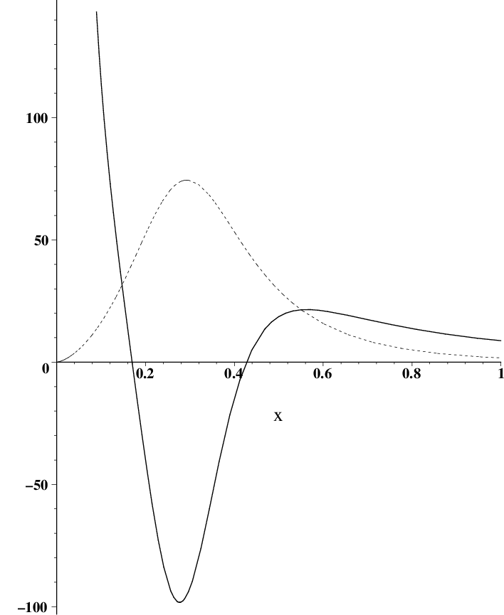
where $A$ and $\alpha$ are arbitrary constants. Note that the $\ell=2$ intertwiner operator constructed using $\psi_{{\cal I}}=\psi_{o}^{+}={\cal A}_{1}\psi^{-}_{o}$ in (64) will depend on $\alpha$ but certainly not on $A$ . It can be easily shown, however, that $\hat{V}$ is smooth at $r=r_{c}$ irrespective of the choice of $\alpha$ , the first and second order poles in $V_{1}^{+}$ being canceled by the poles in $dg/dx$ (Figure 4). This, of course, is to be expected from the more general considerations in Appendix A. The asymptotic behaviour of $\hat{V}$ near the singularity and the inner horizon is also independent of $\alpha$ :

\hat{V}\simeq\begin{cases}\frac{4}{9x{}^{2}}+...&,x\simeq 0\\ C\exp\left(-\frac{(r_{o}-r_{i})x}{r_{i}^{2}}\right)&,x\to\infty\end{cases}

(84)

Near the singularity the eigenfunctions of $\hat{\cal H}$ behave as

\hat{\psi}=A\cos(\theta)[x{}^{-1/3}\;\sum_{n\geq 0}a_{n}^{(1)}x^{n/3}]+A\;\sin(\theta)[x{}^{4/3}\sum_{n\geq 0}a_{n}^{(2)}x^{n/3}]

(85)

Thus $\hat{\cal H}$ belongs to the limit circle case, and only restricting to a subspace ${\cal D}_{\theta_{o}}$ of functions behaving as (85) with a fixed $\theta=\theta_{o}$ value does $\hat{\cal H}$ becomes self-adjoint.
We will make the choice $\theta=\pi/2$ of slowest decaying functions. This condition is certainly preserved by the hat wave equation (see (76)), and implies

\hat{\cal I}\hat{\Phi}=\sum_{k\geq 1}a_{k}r^{k},\;\;\;a_{2}=\frac{\beta_{2}}{4Q^{2}}\,a_{1},

(86)

near $r=0$ . If $\Phi_{1}^{+}(0,r),\dot{\Phi}_{1}^{+}(0,r)$ also admit expansions like those in (86), then, using (74) follows that

\Phi_{1}^{+}(t,r)=\sum_{k\geq 1}a_{k}(t)r^{k},\;\;\;a_{2}(t)=\frac{\beta_{2}}{4Q^{2}}\,a_{1}(t),

(87)

for all $t$ , a condition that can be shown to guarantee that all algebraic invariants of the Riemann tensor behave properly near the singularity.

Regarding the choice of $\alpha$ in (83), although the results do not depend on the intertwiner that we use, it is certainly easier to understand how the instability is excited by an initially compactly bounded perturbation if we use

\tan(\alpha)=\frac{2Q^{2}\,\beta_{2}\,\sqrt{M^{2}-Q^{2}}}{3Q^{2}\beta_{2}\,\ln\left(\frac{M-\sqrt{M^{2}-Q^{2}}}{M+\sqrt{M^{2}+Q^{2}}}\right)+2(3M\beta_{2}-16(M^{2}-Q^{2}))\sqrt{M^{2}-Q^{2}}},

(88)

since in this case the resulting intertwiner will send $\chi_{1}^{+}$ onto the the Hilbert space ${\cal D}_{\pi/2}$ selected by the self consistency argument, and thus ${\cal I}\chi_{1}^{+}$ will be one of the eigenfunctions of $\hat{\cal H}$ (it will actually be the only negative energy $\hat{\cal H}$ eigenfunction). The transformed potential $\hat{V}$ , together with ${\cal I}\chi_{1}^{+}$ for this choice are given in Figure 4 below for some specific $Q$ and $M$ values. An explicit expression for $\hat{V}$ can be readily obtained using equations (64), (67), $\psi_{o}={\cal A}_{1}\psi_{o}^{-}$ , (83) and (88).
Now suppose some perturbation data $(\Phi_{1}^{+}(t=0,x),\dot{\Phi}_{1}^{+}(t=0,x))$ of compact support is given. The hat wave equation data $({\cal I}\Phi_{1}^{+}(t=0,x),{\cal I}\dot{\Phi}_{1}^{+}(t=0,x))$ will be of compact support and then it will belong to ${\cal D}_{\pi/2}$ . Expanding it using (77)-(78) will generically give a nonzero projection onto the fundamental, unstable $\hat{\cal H}$ eigenfunction ${\cal I}\chi_{1}^{+}$ , and thus, from (80), an exponentially growing term in (76), which survives when $\Phi^{+}_{1}$ is reconstructed using (75) and shows up in the metric and electromagnetic field perturbations.

The use of a zero mode intertwiner has some drawbacks: although we can show that the kinematic singularity is absent from $\hat{V}$ (see Appendix B), we do not have a complete proof, even for $\ell=2$ , that the zero mode $\psi_{{\cal I}}=\psi_{o}^{+}$ has no zeroes in $(0,r_{c})\cup(r_{c},r_{i})$ , which would introduce new singularities in $\hat{V}$ . However, for $\ell=2$ , we have numerically verified that this is the case for a range of values of $Q/M$ . A particular example of a smooth $\hat{V}$ for $\ell=2$ is that given in Figure 4.

In the following Section, we show that all these issues can be avoided by using an alternative intertwiner that allows explicit calculations for every harmonic number and charge and mass values.

III.4 Intertwining using Chandrasekhar’s algebraic special mode

We can apply the intertwining technique using Chandrasekhar’s algebraic special mode $\chi_{1}^{+}$ in (64), for which

E_{{\cal I}}=-\left(\frac{\kappa}{2\beta_{1}}\right)^{2}.

(89)

Using this intertwiner has a number of advantages. Contrary to what happens for the zero mode, we have an explicit expression for $\chi_{1}^{+}$ for every harmonic number $\ell$ , equation (26). It is also simple to construct $\hat{V}$ using (7) and (25) (a prime denotes derivative with respect to $x$ ):

\hat{V}=V_{1}^{+}-2\left(\frac{{\chi_{1}^{+}}^{\prime}}{\chi_{1}^{+}}\right)^{\prime}=V_{1}^{+}-\left(\beta_{1}f_{1}+\frac{\kappa}{2\beta_{1}}\right)^{\prime}=V_{1}^{-}=\frac{f}{r^{4}}\left(\ell(\ell+1)r^{2}-\beta_{1}r+4Q^{2}\right)

(90)

(This relation between the scalar and vector modes was first noticed by Chandrasekhar [9, 10].) The fact that $\hat{V}=V_{1}^{-}$ , the type-1 vector potential, simplifies the analysis considerably, since it is clear that $V_{1}^{-}$ is smooth in $(0,r_{i})$ for any value of $Q/M$ .

From the first line in (20) follows that $\hat{\cal H}={\cal H}^{-}_{1}$ belongs to the limit circle case. As explained above, a choice $\theta_{o}$ has to be made to fix the domain ${\cal D}_{\theta_{o}}\subset L^{2}((0,\infty),dx)$ where $\hat{\cal H}$ is self adjoint. However, for type-1 scalar perturbation the consistency requirement (62) (see also Lemma 1) reduces to:

\Big|{\cal I}\Phi_{1}^{+}\Big|\leq N,\;\;\text{ if }\;\;0<r<\delta

(91)

which rules the $x^{-1/3}$ piece of (20), and forces $\theta=\pi/2$ . Once again, this condition is preserved by the hat wave equation (see (76)), and imply (86) and (87) for initial data satisfying this condition (where now ${\cal I}$ has to be understood as the intertwiner made using Chandrasekhar’s mode) Condition (87) guarantees that all algebraic invariants of the Riemann tensor behave properly near the singularity at later times.

Since $\hat{V}$ (and thus $\hat{\cal H}$ ) is positive definite, the hat wave equation is stable, and its modes oscillate in time. The instability of $\Phi_{1}^{+}$ arises as a consequence of the fact that, generically, the exponential terms in the integrand of (74) do not cancel out with those outside the integral. As a trivial example, take $\Phi_{1}^{+}(t=0,x)$ and $\dot{\Phi}_{1}^{+}(t=0,x)$ both proportional to $\chi_{1}^{+}$ (this certainly passes all the requirements in Lemma 1). Since ${\cal I}\chi_{1}^{+}=0$ , the initial data in hat space is trivial, then $\hat{\Phi}(t,x)=0$ for all $t$ , and (74) reduces to the last two terms, which are generically exponentially growing for large $t$ .

A final observation is the nontrivial fact that, unlike the Zerilli field, the intertwined variable has a geometrical significance, as, from (24), it gives the first order variation of the Riemann invariant $R_{1}$ :

{\cal I}\Phi^{+}_{1}=\hat{\Phi}=-\frac{r^{8}}{4Q^{2}}\;\delta R_{1}

(92)

This gives further significance to the dual relation between vector and scalar modes first found by Chandrasekhar, which was limited to some observations on their mode spectra. Equations (24) and (90) prove that the field giving the first order variation of $R_{1}$ (times $Q^{4}/r^{8}$ ) associated to a scalar mode perturbation is a solution of the vector mode perturbation equation of the same harmonic number.

IV Conclusions

We have proved that the inner static region $0<r<r_{i}$ of a Reissner-Nordström black hole is unstable under linear perturbations of the metric and electromagnetic field. More precisely, we have shown that a perturbation with compact support within this region will excite unstable type-1 polar modes, of which there is one for every harmonic number $(\ell,m)$ . This instability is relevant to the strong cosmic censorship conjecture, according to which this region of the black hole, lying beyond the Cauchy horizon (of a Cauchy surface like the one in Figure 1), should be disregarded, as it could not arise as a result of the collapse of ordinary matter departing from spherical symmetry.
This result has implications on some simple models of halted collapse of a pressure-less charged perfect fluid star [25], according to which the world tube of the surface of the star traces a path going from the (right copy of) region I in Figure 1, through region II, into the left copy of region III, upper copy of region II, then upper right copy of region I. To the right of this curve, this spacetime agrees with the extended Reissner-Nordström spacetime, which contains an entire copy of region III, thus being unstable. We are currently studying these models in more detail.
The difficulty in establishing in a rigorous way the Reissner-Nordström instability lies in the fact that the field variable which succeeds in disentangling the linearized equations, the Zerilli field $\Phi_{1}^{+}$ , happens to be a singular function of the perturbed fields in region III. This cannot be cured by any simple field redefinition, but requires the use of an intertwiner operator ${\cal I}=\partial/\partial x+g$ that maps to a smooth field $\hat{\Phi}:={\cal I}\Phi_{1}^{+}$ . The information lost due to the nontrivial kernel of ${\cal I}$ is entirely contained in the initial data, and thus is available. The evolution of perturbations on the non globally hyperbolic background is well defined by using the spectral theorem and a unique self-adjoint extension of the spatial piece of the wave operator that gives the dynamics of the $\hat{\Phi}$ field. We should comment here that intertwiners in the context of linear perturbations were first considered in [24], while they were first used to deal with the issue of the singularities of the Zerilli field in the proof of the instability of the Schwarzschild naked singularity in [4]. The idea of defining dynamics on non globally hyperbolic backgrounds by using a suitable self adjoint extension of the spatial piece of the wave equation together with the spectral theorem was first suggested in [15]. The main difference between the cases considered in [15], and the Reissner-Nordström and negative mass Schwarzschild cases, lies in the fact that the spatial operators (“Hamiltonian”) in the last two cases are not positive definite. A difference between the negative mass Schwarzschild and the Reissner-Nordström cases, is that the intertwiner used in the first case gives a Hamiltonian with a single self-adjoint extension (limit point case in [22]), whereas the one for Reissner-Nordström corresponds to the limit circle case in [22].
Two different intertwiners were used: one constructed out of a zero mode, the other using one of Chandrasekhar’s algebraic special modes. The first intertwiner has the advantage of exhibiting the instability in a rather obvious way, and the drawback that we lack explicit expressions for the interwtined potential, or a proof of its smoothness within the relevant parameter range. The intertwiner that uses Chandrasekhar’s “hides” the instability, which is made explicit in the metric reconstruction process through the original Zerilli field. This mode allows explicit calculations for every harmonic number and $Q$ and $M$ values. It also exhibits a very interesting connection between vector and scalar modes: the intertwined field $\hat{\Phi}$ gives the first order variation of the Riemann invariant $R_{1}$ (see equation (92). An alternative way of stating this is that the first order variation $\delta R_{1}$ of $R_{1}$ under scalar perturbations is a solution of the Zerilli vector perturbation equation.
The results presented here adapt easily to the case of a super-extreme ( $|Q|>M$ ) Reissner-Nordström spacetime, and thus can be used to fill in the details left untreated in [2] to show that a perturbation of an overcharged Reissner-Nordström spacetime, compactly supported away from the singularity, will excite modes that grow exponentially in time. This, of course, is relevant to weak cosmic censorship, this being the original motivation for our work.

Acknowledgements

This work was supported by grants PIP 112-200801-02479 from CONICET (Argentina), Secyt 05/B384 and 05/B253 from Universidad Nacional de Córdoba (Argentina), and a Partner Group grant from the Max Planck Institute for Gravitational Physics, Albert-Einstein- Institute (Germany). RJG and GD are supported by CONICET. GD wishes to thank the AEI, where part of this work was done, for hospitality and support.

Appendix A Intertwined potential

In this section we analyze the local behaviour of the intertwined potential and $\hat{\psi}$ given in equations (64),(65) and (67) as the singularity, inner horizon, and $r=r_{c}$ are approached. This is done by studying the behaviour of generic solutions of the equation

{\cal H}_{1}^{+}\psi_{{\cal I}}=-f\frac{d}{dr}\left(f\frac{d\psi_{{\cal I}}}{dr}\right)+V^{+}_{1}\psi_{{\cal I}}=E_{{\cal I}}\psi^{+}_{1}

(93)

for $r\simeq 0,r\simeq r_{c}$ , and $r\simeq r_{i}$ .

Note that $V^{+}_{1}$ may be written as,

V^{+}_{1}=\frac{f}{r\left(\beta_{1}+(\ell-1)(\ell+2)r\right)^{2}}\;\left[\left(\kappa+\beta_{1}\dfrac{df}{dr}\right)\left(\beta_{1}+(\ell-1)(\ell+2)r\right)-2f(r)\beta_{1}(\ell-1)(\ell+2)\right]

(94)

showing explicitly the double pole at,

r=r_{c}=-\frac{\beta_{1}}{(\ell-1)(\ell+2)}.

(95)

A.1 Behaviour of $\hat{V}$

Near $r=r_{c}$ , the general solution of (93) is of the form,

\psi_{{\cal I}}=\frac{1}{r-r_{c}}\left[c_{0}-\frac{(\ell-1)^{2}(\ell+2)^{2}(2M-\beta_{1})\;c_{0}}{\beta_{1}\left(2(\ell-1)(\ell+2)M+(\ell^{2}+\ell+2)\beta_{1}\right)}(r-r_{c})\right.\\ \left.+\frac{8E_{{\cal I}}\beta_{1}^{2}\;c_{0}}{\left(2(\ell-1)(\ell+2)M+(\ell^{2}+\ell+2)\beta_{1}\right)^{2}}(r-r_{c})^{2}+c_{3}(r-r_{c})^{3}+c_{4}(r-r_{c})^{4}+\dots\right]

(96)

where $c_{0}$ and $c_{3}$ are arbitrary constants, and $c_{4}$ and higher coefficients in the series are linear combinations of $c_{0}$ and $c_{3}$ with coefficients that depend on $E_{{\cal I}},Q,M$ and $\ell$ . Note that the generic local eigenfunction above satisfies the requirement (61).

If we use the generic $\psi_{{\cal I}}$ given above to construct the potential $\widehat{V}$ ,

\widehat{V}=V-2f\frac{d}{dr}\left(\frac{f}{\psi_{{\cal I}}}\frac{d}{dr}\psi_{{\cal I}}\right)

(97)

a straightforward computation shows that, provided $a_{0}\neq 0$ , near $r=r_{c}$ ,

\widehat{V}=\frac{8k^{2}\beta_{1}^{4}+(\ell+2)^{3}(\ell-1)^{3}[(\ell^{2}+\ell+4)\beta_{1}^{2}-20M\beta_{1}-12(\ell+2)(\ell-1)M^{2}]}{4\beta_{1}^{4}}+{\cal{O}}(r-r_{c}).

(98)

This means that, for any $E_{{\cal I}}$ , an arbitrary solution of (93) with $a_{0}\neq 0$ gives an intertwined potential $\widehat{V}$ that is smooth at $r=r_{c}$ . We notice also that, as can be checked, if $a_{0}=0$ , the second term in the R.H.S. of (97) does not compensate the double pole in $V$ , so that $\widehat{V}$ is also singular.

We consider next the local behaviour near $r=0$ . The general solution of (93) admits an expansion in powers of $r$ of the form,

\psi_{{\cal I}}(r)=a_{1}r+a_{2}r^{2}+\left[\frac{(\ell-1)(\ell+2)((\ell-1)(\ell+2)Q^{2}+M\beta_{1})}{Q^{2}\beta_{1}^{2}}a_{1}+\frac{M}{Q^{2}}a_{2}\right]r^{3}+a_{4}r^{4}+\dots

(99)

where $a_{1}$ , and $a_{2}$ are arbitrary constants and the higher order coefficients depend linearly on them. A dependence on $E_{{\cal I}}$ appears first at order $r^{7}$ . This result implies that, near $r=0$ , assuming $a_{1}\neq 0$ , we have,

\widehat{V}=\frac{4}{9}x{}^{-2}-\frac{2}{3^{5/3}}\left(\frac{M}{Q^{4/3}}-\frac{2a_{2}Q^{2/3}}{a_{1}}\right)x{}^{-5/3}+{\cal{O}}(x{}^{-4/3})

(100)

while, if $a_{1}=0$ ,

\widehat{V}=\frac{10}{9}x{}^{-2}+\frac{3^{2/3}}{108}\left(\frac{10\ell(\ell+1)-12)}{Q^{2/3}}+\frac{M(28M-5\beta_{1})}{Q^{8/3}}\right)x{}^{-4/3}+{\cal{O}}(x{}^{-1})

(101)

Finally we consider the behaviour near $r=r_{i}$ . The cases $E_{{\cal I}}\neq 0$ and $E_{{\cal I}}=0$ require separate treatment. For $E_{{\cal I}}\neq 0$ , since the potential vanishes for $r=r_{i}$ , the leading terms of the two linearly independent parts of the solution for real $E_{{\cal I}}$ are of the form,

	$\displaystyle\psi_{{\cal I}}$	$\displaystyle=$	$\displaystyle C_{1}(r_{i}-r)^{\left(\dfrac{r_{i}^{2}\sqrt{E_{{\cal I}}}}{r_{o}-r_{i}}\right)}+C_{2}(r_{i}-r)^{\left(\dfrac{-r_{i}^{2}\sqrt{E_{{\cal I}}}}{r_{o}-r_{i}}\right)}$		(102)
		$\displaystyle=$	$\displaystyle\tilde{C}_{1}\exp\left(\sqrt{E_{{\cal I}}}x\right)+\tilde{C}_{2}\exp\left(-\sqrt{E_{{\cal I}}}x\right)$		(102)

where $C_{1}$ , $C_{2}$ , $\tilde{C}_{1}$ , and $\tilde{C}_{2}$ are constants. For $E_{{\cal I}}=0$ , on the other hand, the general solution admits an expansion of the form,

$\displaystyle\psi_{1}^{+}(r)$	$\displaystyle=$	$\displaystyle a_{0}+\frac{\left((r_{i}-r_{o})\beta_{1}+\kappa r_{i}^{2}\right)a_{0}-r_{i}\left(\beta_{1}+(\ell+2)(\ell-1)((2\ell^{2}+2\ell-1)r_{i}+2r_{o})\right)b_{0}}{r_{i}(r_{i}-r_{o})(\beta_{1}+r_{i}(\ell+2)(\ell-1))}(r-r_{i})$	(103)
		$\displaystyle+a_{2}(r-r_{i})^{2}+\dots$
		$\displaystyle+\ln(r_{i}-r)\left[b_{0}+\frac{\left((r_{i}-r_{o})\beta_{1}+\kappa r_{i}^{2}\right)b_{0}}{r_{i}(r_{i}-r_{o})(\beta_{1}+r_{i}(\ell+2)(\ell-1))}(r-r_{i})+b_{2}(r-r_{i})^{2}+\dots\right].$

where $a_{2}$ , $b_{2}$ and higher order coefficients depend linearly on $a_{0}$ and $b_{0}$ .
The $E_{{\cal I}}=0$ transformed potential behaves as

\widehat{V}(r)=\frac{2(r_{o}-r_{i})^{2}b_{0}^{2}}{(a_{0}+b_{0}\ln(r_{i}-r))^{2}r_{i}^{4}}+\dots

(104)

where the dots indicate terms that vanish as a $(r_{i}-r)$ . In terms of $x$ , for $b_{0}\neq 0$ , this implies,

\widehat{V}(x)=\frac{2}{x^{2}}+\dots

(105)

A.2 Behaviour of $\hat{\psi}$

We consider now the behaviour of the intertwined field $\widehat{\psi}$ (64), which can be written as

\widehat{\psi}={\cal I}\psi=f\psi_{{\cal I}}\frac{d}{dr}\left(\frac{\psi}{\psi_{{\cal I}}}\right).

(106)

We will use the following result, whose proof is straightforward:

Lemma 2: Assume that $\psi$ and $\psi_{{\cal I}}$ admit a Laurent expansion

\psi=(r-r_{o})^{p}\;\sum_{k\geq 0}a_{k}\;(r-r_{o})^{k},\;\;\;\psi_{{\cal I}}=(r-r_{o})^{p}\;\sum_{k\geq 0}a_{k}^{{\cal I}}\;(r-r_{o})^{k}

(107)

where $a_{0}=1=a_{0}^{{\cal I}}$ , and $p$ is any integer number. If $s$ is the highest number for which $a_{k}=a_{k}^{{\cal I}}$ for every $k\leq s$ ( $s$ measures the degree of contact of these functions at $r_{o}$ , and, generically, $s=0$ ), then

\psi_{{\cal I}}\frac{d}{dr}\left(\frac{\psi}{\psi_{{\cal I}}}\right)=(r-r_{o})^{p}\;\sum_{k\geq s}d_{k}(r-r_{o})^{k},\;\;d_{s}=s(a_{s+1}-a_{s+1}^{{\cal I}}).

(108)

Consider first the action of the intertwiner on a function $\psi$ satisfying (58) and (61). Since, as follows from (96), $\psi_{I}$ satisfies this same condition, generically $\psi$ and $\psi_{{\cal I}}$ have (as functions of $r$ ) degree of contact $s=2$ , in the notation of Lemma 2, and thus $\hat{\psi}=f\psi_{{\cal I}}\frac{d}{dr}\left(\frac{\psi}{\psi_{{\cal I}}}\right)$ will be smooth at $r=r_{c}$ .

The local solutions of ${\cal H}^{+}_{1}\psi=E\psi$ , are of the form $\psi=\sum_{k\geq 1}a_{k}r^{k}$ with $a_{2}$ and $a_{1}$ arbitrary, $a_{k}$ independent of $E$ up to $k=7$ . Consider the action of ${\cal I}$ on a function like this further subject to the condition (86). If the intertwiner also satisfies (86), the degree of contact will be $s=5$ , then $\psi_{{\cal I}}\frac{d}{dr}\left(\frac{\psi}{\psi_{{\cal I}}}\right)$ will be ${\cal O}(r^{6})$ , and thus $\hat{\psi}$ will be ${\cal O}(r^{4})={\cal O}(x^{4/3})$ .

Appendix B The scalar and vector zero modes.

In this Appendix we describe a procedure that allows the construction of the zero mode solutions for both vector and scalar modes. We start with the vector zero modes by first considering the differential equation they satisfy. In accordance with (6, 7), and (9) with $\omega=0$ , this is given by,

-f^{2}\frac{d^{2}\psi^{-}_{0}}{dr^{2}}-f\frac{df}{dr}\frac{d\psi^{-}_{0}}{dr}+\frac{f}{r^{4}}\left(\ell(\ell+1)r^{2}-\beta_{1}r+4Q^{2}\right)\psi^{-}_{0}=0

(109)

We notice that (109) has regular singular points for $r=0$ , $r=r_{i}$ and $r=r_{o}$ , and no other singularity. From now on we will write simply $\psi$ for $\psi_{0}^{-}$ .

A simple analysis of the indicial equation shows that near $r=0$ this equation has two independent solutions, one behaving as $r^{-1}$ , and the other as $r^{4}$ , both admitting a power series expansion. We consider therefore an expansion for $\psi^{-}_{0}(r)$ of the form,

\psi^{-}_{0}(r)=\frac{1}{r}\sum_{i=0}^{\infty}{a_{i}r^{i}}

(110)

Replacing in (109) we find that we must set $a_{2}=0$ , and,

a_{1}=-\frac{\beta_{2}}{4Q^{2}}a_{0}\;\;;\;\;a_{3}=\frac{\ell(\ell+1)\beta_{2}}{24Q^{4}}a_{0}\;\;;\;\;a_{4}=\frac{\ell(\ell^{2}-1)(\ell+2)}{24Q^{4}}a_{0}

(111)

The coefficient $a_{5}$ can be chosen arbitrarily, in accordance with the indicial equation, and $a_{6}$ is given by,

a_{6}=-\frac{\ell(\ell^{2}-1)(\ell^{2}-4)(\ell+3)}{144Q^{6}}a_{0}-\frac{\beta_{1}-16M}{6Q^{2}}a_{5}

(112)

For the remaining coefficients, including $a_{6}$ , we find a three term recursion relation of the form,

-(\ell+j-2)(\ell-j+3)a_{j-1}+(\beta_{1}-2(j-1)(j-3)M)a_{j}+(j+1)(j-4)Q^{2}a_{j+1}=0

(113)

and, therefore, all the coefficients are determined once $a_{0}$ , and $a_{5}$ are given. But this implies that for any given $\ell$ , and $a_{0}\neq 0$ , we may choose $a_{5}$ such that $a_{\ell+3}=0$ , and then all coefficients for $j\geq\ell+3$ vanish. Calling $\psi_{a}$ this solution we have,

\psi_{a}(r)=\frac{1}{r}{\cal{P}}_{\ell}(r)

(114)

where ${\cal{P}}_{\ell}(r)$ is a polynomial of order $\ell+2$ . The lowest order polynomials are,

$\displaystyle{\cal{P}}_{2}(r)$	$\displaystyle=$	$\displaystyle 1-\frac{\beta_{2}}{4Q^{2}}r+\frac{\beta_{2}}{4Q^{4}}r^{3}-\frac{1}{Q^{4}}r^{4}$
$\displaystyle{\cal{P}}_{3}(r)$	$\displaystyle=$	$\displaystyle 1-\frac{\beta_{2}}{4Q^{2}}r+\frac{\beta_{2}}{2Q^{4}}r^{3}-\frac{5}{Q^{4}}r^{4}+\frac{30}{(\beta_{2}+10M)Q^{4}}r^{5}$	(115)
$\displaystyle{\cal{P}}_{4}(r)$	$\displaystyle=$	$\displaystyle 1-\frac{\beta_{2}}{4Q^{2}}r+\frac{5\beta_{2}}{6Q^{4}}r^{3}-\frac{15}{Q^{4}}r^{4}+\frac{21(24M+\beta_{2})}{4(3Q^{2}+M\beta_{2}+6M^{2})Q^{4}}r^{5}-\frac{42}{(3Q^{2}+6M^{2}+M\beta_{2})Q^{4}}r^{6}$

where we have fixed, for simplicity, ${\cal{P}}_{\ell}(r=0)=1$ . With this normalization, the polynomials are positive and decreasing functions of $r$ near $r=0$ . We shall now prove that they have no zeros in the interval $0\leq r\leq r_{i}$ . We write (109) in the form,

\frac{d^{2}\psi_{a}}{dr^{2}}=\frac{(2r_{i}r_{o}-(r_{i}+r_{o})r)}{r(r_{o}-r)(r_{i}-r)}\frac{d\psi_{a}}{dr}+\frac{(\ell(\ell+1)r^{2}-\beta_{1}r+4r_{i}r_{o})}{r^{2}(r_{o}-r)(r_{i}-r)}\psi_{a}

(117)

and notice that $\psi_{a}$ can have only simple zeros in $0<r<r_{i}$ because the coefficients in (117) are regular functions of $r$ in $0<r<r_{i}$ . Since sufficiently near $r=0$ we have $\psi_{a}>0$ and $d\psi_{a}/dr<0$ , and the coefficients on the RHS in (117) are both positive, the sign of $d^{2}\psi_{a}/dr^{2}$ is not fixed. We notice however that at the first zero of $\psi_{a}$ for $r>0$ we must have $d\psi_{a}/dr<0$ , and therefore, we also have $d^{2}\psi_{a}/dr^{2}<0$ . Since to the right of such a zero, and as long as $r<r_{i}$ , (since the coefficients are still positive) we must have both $d\psi_{a}/dr<0$ , and $d^{2}\psi_{a}/dr^{2}<0$ , and therefore $\psi_{a}<0$ , there can be no other zero for $r<r_{i}$ . This proves that there is at most one zero for $r\in(0,r_{i})$ .
But now we notice that near $r=r_{i}$ , equation (117) has a singular solution (diverging as $\ln(r_{i}-r)$ ) and a unique regular solution of the form,

\psi(r)=\psi(r_{i})\left[1-\frac{(4r_{o}+\ell(\ell+1)r_{i}-\beta_{1})}{r_{i}(r_{o}-r_{i})}(r-r_{i})+{\cal{O}}(r-r_{i})^{2}\right]

(118)

Since $\psi_{a}$ is regular, it has the form (118), and this implies that close to $r=r_{i}$ the regular solution and its first derivative have opposite signs. This contradicts the result obtained under the assumption that there is a zero in $0<r<r_{i}$ . We conclude that $\psi_{a}$ does not vanish for $r\in(0,r_{i})$ .
Similarly, we find that near $r=r_{o}$ , equation (117) has a singular solution (diverging as $\ln(r_{o}-r)$ ) and a unique non vanishing regular solution. This implies that ${\cal{P}}_{\ell}(r)$ cannot vanish for $r=r_{o}$ .

We note in passing that for the extreme case $Q=M$ , where $r_{i}=r_{o}$ , we have the exact (regular at the horizon) solutions,

\psi_{a}(r)=\frac{C(\ell r+2M)(r-M)^{(\ell+1)}}{r}

(119)

where $C$ is a constant.
Going back to (109), for any fixed $\ell$ , given the solution (114), a linearly independent solution is given by,

\psi_{b}(r)=C\frac{1}{r}{\cal{P}}_{\ell}(r)\int_{0}^{r}\frac{y^{4}}{(y^{2}-2My+Q^{2})\left({\cal{P}}_{\ell}(y)\right)^{2}}dy

(120)

where $C$ is a constant. It is easy to check that $\psi_{b}$ is regular and non vanishing in $0<r<r_{i}$ , and,

	$\displaystyle\psi_{b}(r)$	$\displaystyle\sim$	$\displaystyle C_{1}r^{4}\;\;;\;\;r\to 0^{+}$
	$\displaystyle\psi_{b}(r)$	$\displaystyle\sim$	$\displaystyle C_{2}\ln(r_{i}-r)\;\;;\;\;r\to r_{i}{}^{-}$		(121)

where $C_{1}$ and $C_{2}$ are constants. We may obtain and expansion of this solution in powers of $r$ using (120), or directly from (109),

	$\displaystyle\psi_{b}(r)$	$\displaystyle=$	$\displaystyle r^{4}+\frac{(16M-\beta_{1})r^{5}}{6Q^{2}}+\frac{5((\ell^{2}+\ell-8)Q^{2}+4M(12M-\beta_{1}))r^{6}}{42Q^{4}}$		(122)
			$\displaystyle+\frac{((\ell(\ell+1)(36M-\beta_{1})+15\beta_{1}-360M)Q^{2}+30M^{2}(32M-3\beta_{1}))r^{7}}{84Q^{6}}+\dots$		(122)

where we have set an arbitrary multiplicative constant so that the coefficient of $r^{4}$ is equal to one.

For $\ell>2$ the integrals in (120) cannot be computed directly, because that would require explicit expressions for the zeros of polynomials of degree larger that 4. We may, nevertheless, infer their general form as follows. We first notice that ${\cal{P}}_{\ell}(r)$ may be written in the form,

{\cal{P}}_{\ell}(r)=\frac{\prod_{k=1}^{\ell+2}(r-r_{k})}{\prod_{k=1}^{\ell+2}(-r_{k})}

(123)

where $r_{k}$ are the zeros of ${\cal{P}}_{\ell}(r)$ , which, as indicated are simple. Therefore, since $y^{2}-2My+Q^{2}=(y-r_{i})(y-r_{o})$ , we should have,

	$\displaystyle\int_{0}^{r}\frac{y^{4}}{(y^{2}-2My+Q^{2})\left({\cal{P}}_{\ell}(y)\right)^{2}}dy$	$\displaystyle=$	$\displaystyle A\ln(r_{i}-r)+B\ln(r_{o}-r)+C$		(124)
			$\displaystyle+\sum_{k=1}^{\ell+2}a_{i}\ln(r-r_{k})+\sum_{k=1}^{\ell+2}{\frac{b_{i}}{(r-r_{k})}}$		(124)

where $A$ , $B$ , $C$ , $a_{k}$ and $b_{k}$ are constants that depend on $M$ , $Q$ , and $r_{k}$ . The last term in (124) may be written in the form,

\sum_{k=1}^{\ell+2}{\frac{b_{i}}{(r-r_{k})}}=\frac{U_{\ell}(r)}{{\cal{P}}_{\ell}(r)}

(125)

where $U_{\ell}(r)$ is a polynomial of order $\ell-1$ , or lower. Replacing in (120),

	$\displaystyle\psi_{b}(r)$	$\displaystyle=$	$\displaystyle\frac{1}{r}{\cal{P}}_{\ell}(r)\left(A\ln(r_{i}-r)+B\ln(r_{o}-r)+C\right)+\frac{1}{r}{U}_{\ell}(r)$		(126)
			$\displaystyle+\frac{1}{r}{\cal{P}}_{\ell}(r)\sum_{k=1}^{\ell+2}a_{i}\ln(r-r_{k})$		(126)

But we notice that $\psi_{b}(r)$ is a solution of (109), which can be singular only at the regular singular points $r=0$ , $r=r_{i}$ , and $r=r_{o}$ , and that the zeros $r_{k}$ do not coincide with these points. Therefore, we must have $a_{k}=0$ for all $k$ , and the last term in (126) vanishes identically. This result implies that, for any $\ell$ , we may construct algebraically the solution (120) as follows. We first compute the coefficients of ${\cal{P}}_{\ell}(r)$ as indicated above, and then replace in (126) leaving $A$ , $B$ , $C$ and the coefficients of $U_{\ell}$ arbitrary. Next we replace in (109) and impose the condition that $\psi$ is a solution of that equation, and that $\psi\sim r^{4}$ near $r=0$ . It can be checked that this procedure determines all the coefficients, up to an arbitrary multiplicative constant, a simple example being (83) for $\ell=2$ . Since by construction these solutions satisfy the appropriate boundary condition at $r=0$ , the construction of the corresponding scalar zero modes, and the associated intertwining potential, is now a simple algebraic procedure. The resulting expressions are, unfortunately, very long and rather difficult to analyze in detail. In particular, we have not been able to show explicitly that for $0<r_{c}<r_{i}$ the scalar zero modes that satisfy the required boundary condition at $r=0$ are non vanishing everywhere in the interval $0<r<r_{i}$ , as required for the regularity of the intertwining potential. We remark, nevertheless, that this appears to be the case in all the particular solutions analyzed numerically after assigning definite numerical values for the parameters, as in the example described in Section III - C.

References

[1] R. J. Gleiser and G. Dotti, Class.Quant.Grav.23, 5063 (2006) [arXiv:gr-qc/0604021]
[2] G.Dotti, R. J. Gleiser, J. Pullin Phys.Lett. B644 (2007) 289-293 [arXiv:gr-qc/0607052]
[3] G. Dotti, R. J. Gleiser, I. F. Ranea-Sandoval and H. Vucetich, Class. Quant. Grav. 25, 245012 (2008), arXiv:0805.4306 [gr-qc].
[4] G. Dotti and R.J. Gleiser, Class.Quant.Grav.26, 215002 (2009), arXiv:0809.3615 [gr-qc]
[5] G. Dotti, R. J. Gleiser, J. Pullin, I. F. Ranea-Sandoval and H. Vucetich, Instabilities of naked singularities and black hole interiors in General Relativity, talk given at the 7th Alexander Friedmann International Seminar on Gravitation and Cosmology, Joao Pessoa, Brazil, 29 Jun - 5 Jul 2008. Int. J. Mod. Phys. A 24, 1578 (2009), [arXiv:0810.0025 [gr-qc]].
[6] Gibbons G W, Hartnoll D and Ishibashi A 2005 Prog.Theor.Phys. 113 963-978, hep-th/0409307.
[7] V. Cardoso and M. Cavaglia, Phys.Rev. D74, 024027 (2006) [arXiv:gr-qc/0604101]; V. Cardoso, P. Pani, M. Cadoni and M. Cavaglia, Class. Quant. Grav. 25, 195010 (2008) [arXiv:0808.1615 [gr-qc]]; V. Cardoso, O. J. C. Dias and S. Yoshida, Phys. Rev. D 74, 044008 (2006) [arXiv:hep-th/0607162]; V. Cardoso, P. Pani, M. Cadoni and M. Cavaglia, Class. Quant. Grav. 25, 195010 (2008) [arXiv:0808.1615 [gr-qc]];
[8] V. Cardoso, O. J. C. Dias and S. Yoshida, Phys. Rev. D 74, 044008 (2006) [arXiv:hep-th/0607162].
[9] S. Chandrasekhar Proc. Roy. Soc. Lond. A 392, 1 (1983).
[10] S. Chandrasekhar, The Mathematical Theory of Black Holes, Oxford University Press, 1992.
[11] V. Moncrief, Phys. Rev. D 10, 1057 (1974).
[12] T. Regge, J. Wheeler, Phys. Rev. 108, 1063 (1957). F. J. Zerilli, Phys. Rev. Lett. 24 737 (1970), Phys. Rev. D2, 2141 (1970), Phys. Rev. D9, 2141 (1974).
[13] H. Kodama and A. Ishibashi, Prog. Theor. Phys. 110, 901 (2003) [arXiv:hep-th/0305185]; Prog. Theor. Phys. 110, 701 (2003) [arXiv:hep-th/0305147]; Phys. Rev. D 62, 064022 (2000) [arXiv:hep-th/0004160];
[14] H. Kodama and A. Ishibashi, arXiv:gr-qc/0312012; Prog. Theor. Phys. 111, 29 (2004) [arXiv:hep-th/0308128].
[15] R.M. Wald, J. Math. Phys. 21, 2802 (1980); A. Ishibashi and R. M. Wald, Class. Quant. Grav. 20, 3815 (2003) [arXiv:gr-qc/0305012]; Class. Quant. Grav. 21, 2981 (2004) [arXiv:hep-th/0402184]
[16] R. Penrose, Riv. del Nuovo Cim. 1 (numero speziale) (1969), 252–276
[17] J. Carminati and R. G. McLenaghan, J. Math. Phys. 32, 3135 (1991)
[18] M. Simpson and R.Penrose, Internatl. J. Theor. Phys. 7 (1973), 183.
[19] E. Poisson and W. Israel, Phys. Rev. D 41 (1990), 1796.
[20] M. Dafermos, “Stability and Instability of the Reissner-Nördstrom Cauchy Horizon and the Problem of Uniqueness in General Relativity,” arXiv:gr-qc/0209052; M. Dafermos, The Annals of Mathematics, Second Series, Vol. 158, No. 3 (2003), 875.
[21] See http://grtensor.phy.queensu.ca/
[22] M. Reed and B. Simon, Methods of modern mathematical physics (v. 2: Fourier analysis, self-adjointness), section X, Academic Press (1975); R. Rytchmyer, Principles of advanced mathematical physics, Springer (1978); K. Meetz, Il Nuovo Cimento 34 690 (1964).
[23] K. M. Case, Phys. Rev 80, 797 (1950).
[24] A. Anderson and R. H. Price, Phys. Rev. D 43, 3147 (1991).
[25] J.D. Bekenstein, Phys. Rev. D 4, 2185 (1971); V. de la Cruz and W. Israel, Il Nuovo Cimento 51A 744 (1967); I. Novikov, Sov. Astron. AJ 10 731 (1967); A. Ori, Class. Quant. Grav. 7, 985 (1990).

Gravitational instability of the inner static region of a Reissner-Nordström black hole

Abstract

pacs

I Introduction

II Linear perturbations of a Reissner-Nordström black hole

II.1 The Reissner-Nordström spacetime and its maximal analytic extension

II.2 Linearized gravity around the Reissner-Nordström solution

II.3 Consistency of the linearized analysis

II.4 Factorization of Zerilli’s Hamiltonian and algebraic special modes

II.4.1 Algebraic special vector modes

II.4.2 Algebraic special scalar modes

III Proof of the linear instability of the inner static region

III.1 Basics of the intertwining technique

III.2 The initial value problem for perturbations of region III

III.3 The ℓ=2\ell=2 zero mode intertwiner

III.4 Intertwining using Chandrasekhar’s algebraic special mode

IV Conclusions

Acknowledgements

Appendix A Intertwined potential

A.1 Behaviour of V^\hat{V}

A.2 Behaviour of ψ^\hat{\psi}

Appendix B The scalar and vector zero modes.

References

III.3 The $\ell=2$ zero mode intertwiner

A.1 Behaviour of $\hat{V}$

A.2 Behaviour of $\hat{\psi}$