General CMB and Primordial Bispectrum Estimation I:
Mode expansion, map-making
and measures of
Abstract
We present a detailed implementation of two parallel bispectrum estimation methods which can be applied to general non-separable primordial and CMB bispectra. The method exploits bispectrum mode decompositions on the tetrahedral domain of allowed wavenumber or multipole values, using both separable basis functions and related orthonormal modes. We provide concrete examples of such modes constructed from symmetrised tetrahedral polynomials, demonstrating the rapid convergence of expansions describing nonseparable bispectra. We use these modes to create rapid and robust pipelines for generating simulated CMB maps of high resolution () given an arbitrary primordial power spectrum and bispectrum or an arbitrary late-time CMB angular power spectrum and bispectrum. By extracting coefficients for the same separable basis functions from an observational map, we are able to present an efficient estimator for a given theoretical model with a nonseparable bispectrum. The estimator has two manifestations, comparing the theoretical and observed coefficients at either primordial or late times, thus encompassing a wider range of models, including secondary anisotropies and lensing as well as active models, such as cosmic strings. We provide examples and validation of both estimation methods by direct comparison with simulations in a WMAP-realistic context. In addition, we demonstrate how the full primordial and CMB bispectrum can be extracted from observational maps using these mode expansions, irrespective of the theoretical model under study. We also propose a universal definition of the bispectrum parameter , so that the integrated bispectrum on the observational domain can be more consistently compared between theoretical models. We obtain WMAP5 estimates of for the equilateral model from both our primordial and late-time estimators which are consistent with each other, as well as results already published in the literature. These general bispectrum estimation methods should prove useful for nonGaussianity analysis with the Planck satellite data, as well as in other contexts.
I Introduction
Standard inflationary scenarios predict the Universe to be close to flat with primordial curvature perturbations which are nearly scale-invariant and Gaussian. All these predictions are in very good accord with cosmic microwave background (CMB) and large-scale structure measurements, such as those provided by WMAP and SDSS. Despite this remarkable agreement, present observations are not able to completely rule out alternatives to inflation, nor to effectively discriminate among the vast number of different inflationary models that have been proposed. However, almost all such quantitative comparisons derive from inferred measurements of the primordial two-point correlator or power spectrum from , where is the curvature perturbation. If we wish to subject inflation to more stringent tests and to distinguish between competing models then perhaps the best prospects are offered by studying nonGaussianity, that is, the higher order correlators beyond the power spectrum. The three-point correlator of the CMB or bispectrum is a projection on the sky of the evolved primordial bispectrum arising from , consisting of contributions from triangle configurations with sidelengths given by the wavenumbers . The bispectrum has attracted most attention in the literature to date and its study is usually simplified to the characterization of a single nonlinearity parameter , which schematically is given by the ratio .
Standard inflation, that is, single field slow-roll inflation, predicts a very small bispectrum with [1, 2], possessing a characteristic scale-invariant local shape. (This local shape is dominated by squeezed triangle configurations, that is, those for which one side is much smaller than the others, e.g. .) In fact, such a low signal would be undetectable even by an ideal noiseless CMB experiment, because it is below the level of NG contamination expected from secondary anisotropies . However, measurement of a significantly larger primordial would have profound consequences because it would signal the need for new physics during inflation or even a paradigm shift away from it. Present measurements of this local are equivocal with the WMAP team reporting [3]
| (1) |
and with other teams obtaining higher [4] (WMAP3) or equivalent values [5, 6], while with improved WMAP5 noise analysis a lower value was found , but at a similar 2 significance [7]. The Planck satellite experiment is expected to markedly improve precision measurements with or better [8].
Further motivation for the study of the bispectrum comes from the prospect of distinguishing alternative more complex models of inflation which can produce nonGaussianity with potentially observable amplitudes , but also in a variety of different bispectrum shapes, that is, with the nonGaussian signal peaked for different triangle configurations of wavevectors. To date only special separable bispectrum shapes have been constrained by CMB data, that is, those that can be expressed (schematically) in the form , or else can be accurately approximated in this manner. All CMB analysis, such as those quoted above for the local shape (1), exploits this separability to reduce the dimensionality of the required integrations and summations to bring them to a tractable form. The separable approach reduces the problem from one of operations to a manageable [9]. Other examples of meaningful constraints on separable bispectrum shapes using WMAP5 data include those for the equilateral shape [3] and another shape ‘orthogonal’ to both equilateral and local [10]. Despite these three shapes being a good approximation to non-Gaussianity from a number of classes of inflation models, they are not exhaustive in their coverage of known primordial models [11], nor other types of late-time non-Gaussianity, such as that from cosmic strings [12, 13]; they cannot be expected to be, given the functional degrees of freedom available. Bringing observations to bear on this much broader class of cosmological models, therefore, is the primary motivation for this paper.

In a previous paper [14], we described a general approach to the estimation of non-separable CMB bispectra. The method has developed out of the first direct calculations of the reduced CMB bispectrum which surveyed a wide variety of non-separable primordial models, revealing smooth coherent patterns of acoustic peaks on the tetrahedral domain of allowed multipole values. Since the could be well represented using a limited number of bins, we could similarly decompose them into orthogonal mode functions which converged in relatively short mode expansions [11]. Here, we describe the detailed implementation of these methods in a comprehensive dual approach to estimating bispectrum parameters which is illustrated in fig. 1. We present concrete examples of separable basis functions (symmetrised tetrahedral polynomials) and corresponding orthonormal modes on the domain of allowed wavenumbers ; these are then deployed within a more general mode expansion methodology. In the first primordial implementation, we decompose an arbitrary non-separable shape using separable basis functions with coefficients . This expansion can be used for a fast calculation of the full CMB bispectrum (section III), as well as leading to a robust method for generating simulated maps from a given power spectrum and bispectrum (section IV). Our main emphasis here, however, is on a primordial estimator for which is achieved by a confrontation between theory, represented by the coefficients, and a set of observational coefficients found by extracting the same modes from the observed CMB map (section III). Examples of simulated maps and recovery of the input are given in section V in a WMAP-realistic context.
In the second and parallel late-time implementation (see fig. 1), we assume the theoretical CMB bispectrum is calculated already from the primordial shape [11] or because it is a late-time effect ranging from secondary anisotropies through to fluctuations induced by cosmic strings. A separable mode expansion of allows for a simpler and more direct approach to estimation, as well as simulated map generation, in a wider variety of scenarios. Here, as well as primordial models we consider the antithetical example of cosmic strings. These two estimator methods are complementary with each having distinct advantages depending on the properties and generation mechanism of the non-Gaussianity under investigation. They provide independent validation in situations where both are applicable.
It remains to point out recent and related developments, especially those by colleagues in Planck Working Group 4 (NonGaussianity). To date most primordial shapes have been assumed to be scale-invariant, but in ref. [15] some deviations from the local shape were considered in developing a more general approach. Spherical Mexican wavelets, using a limited number of scales, were employed in ref. [5, 16] to estimate for the local shape with WMAP3 data, providing a constraint consistent with (1). Similar work has been achieved for needlets with corresponding constraints [6]), again essentially tailoring the method to the local template using local shape map simulations. Another approach to a late-time estimator has also exploited the smoothness of the reduced CMB bispectrum by using a limited number of multipole bins [17]. The method was tested for the local shape using map simulations, and emphasised Planck forecasts investigating the pattern of acoustic peaks in the local model. We shall discuss here how these late time approaches – whether wavelets, bins or other alternatives – fall within the general mode expansion methodology outlined previously [14] and can be applied, in principle, to explore nonseparable primordial models beyond local nonGaussianity. We point out in the implementation presented here, however, that direct estimation of the CMB bispectrum can be achieved without reference to the calculated bispectrum for a particular model and without relying on corresponding CMB map simulations.
II The CMB bispectrum and estimation
II.1 Relation between primordial and CMB bispectra
In this section we will review some basic definitions and mathematical formulae that will be used throughout the rest of the paper. Our work will be concerned with the analysis of the three-point function induced by a NG primordial gravitational potential in the CMB temperature fluctuation field. Temperature anisotropies are represented using the coefficients of a spherical harmonic decomposition of the cosmic microwave sky,
The primordial potential is imprinted on the CMB mutipoles by a convolution with transfer functions representing the linear perturbation evolution, through the integral
| (2) |
The CMB bispectrum is the three point correlator of the , so substituting we obtain
| (3) | |||||
| (5) | |||||
where , and . Here, we define the primordial bispectrum as
| (6) |
where the delta function enforces the triangle condition, that is, the constraint imposed by translational invariance that wavevectors in Fourier space must close to form a triangle, . We replace the delta function in (6) with its exponential integral form, substitute this into equation (3) and integrate out the angular parts of the three integrals in the usual manner to yield
| (7) |
The last integral over the angular part of is known as the Gaunt integral which can be expressed in terms of Wigner- symbols as
Given that most theories we shall consider are assumed to be isotropic, it is usual to work with the angle-averaged bispectrum,
or the even more convenient reduced bispectrum which removes the geometric factors associated with the Gaunt integral,
| (14) |
The reduced bispectrum from (3) then takes the much simpler form
| (15) |
Here, it is important to note that the Gaunt integral in (14) encodes several constraints on the angle averaged bispectrum which are no longer transparent in the reduced bispectrum . These are, first, that the sum of the three multipoles must be even and, secondly, that the ’s satisfy the triangle condition, analogously to the wavenumbers . For wavenumbers, the triangle condition is enforced through the -integral over the three spherical Bessel functions which evaluates to zero if the ’s cannot form a triangle, whereas in multipole space it is enforced by the angular integration over the spherical harmonics in (II.1). Appreciating the origin of these constraints is important when we later consider the separability of the reduced bispectrum expression (7).
II.2 Separable primordial shapes and CMB bispectrum solutions
Given that the primordial power spectrum is very nearly scale-invariant, it is expected that the bispectrum will behave similarly. In order to bring the bispectrum to a scale-invariant form we have to appropriately eliminate a scaling which naturally arises in (6). This is usually achieved by multiplying through by the factor appearing in (15) and defining a primordial shape function as
| (16) |
where is a normalisation factor which is often taken such that for equal the shape function has unit value . (This normalisation is also used for , but it only strictly applies for scale-invariance and, in any case, leads to inconsistent comparisons between different models, as we shall discuss in section IV.) We thus characterise scale-invariant models in terms of an overall amplitude, parametrised by , and their transverse shape, described by on a triangular slice with [18]. This leaves a two-dimensional space on which it is most elegant to use the two independent variables [19, 14]
| (17) |
with the following domains and . For scale-dependent models with a non-trivial variation in , the full three-dimensional dependence on the must be retained. In terms of the shape function (16), the reduced bispectrum (15) can be rewritten as
| (18) |
The simplest possible shape function is the constant model
| (19) |
for which a large-angle analytic solution for the reduced bispectrum was presented in ref. [11],
| (20) |
Here, we take the Sachs-Wolfe approximation that for and exploit the manifest separability of the expression (18) to perform the one-dimensional integrations individually. The more general constant solution does not have an analytic solution for , for the reason that the transfer functions cannot be expressed in a simple form, but it can be evaluated numerically from the expression
| (21) |
The large-angle solution (20) is an important benchmark with which to compare the shape of late-time CMB bispectra from other models (note the scaling) and, additionally, it has some further recent physical motivation [20].
The most studied scale-invariant shape function is the local model,
| (22) | |||||
where, in the second line, we also allow for power spectra which are nearly scale invariant, defined by with . Using the Sachs-Wolfe approximation again, this has the corresponding large-angle analytic solutions
| (23) |
Here, we see that the divergences for the squeezed triangles () in the primordial shape (22) are also reflected in , making it a much less useful for relative comparison than the constant model (20). It is straightforward, in principle, to calculate the full bispectrum from the separable expressions arising from (22),
| (24) |
where the separated integrals analogous to (21) become
| (25) |
We note that these highly oscillatory integrals must be evaluated numerically with considerable care.
The separable equilateral shape has also received a great deal of attention with [18]
| (26) | |||||
This is a much more regular shape than local (22) with the signal dominated by equilateral triangle configurations (the apparent divergence of the local shape in the second term cancels against the third). There is no simple large-angle analytic solution known for the equilateral model, unlike (21) and (24). In order to calculate the full equilateral bispectrum we evaluate the simplified expression
| (27) |
where are given in (25) and are defined by
| (28) |
The equilateral shape is not derived directly from a physical model, but was chosen phenomenologically as a good separable approximation to specific models including the non-local part of Maldacena’s original shape [1], as well as non-canonical cases such as higher derivative models [21] and DBI inflation [22] (for a review of single-field inflation shapes, see e.g. ref. [23]). These shapes are, in general, non-separable from the perspective of the integral (18). Here, we give a specific shape example for a model with higher derivative operators (which is also identical to DBI inflation):
| (29) |
Not only is the equilateral shape (26) an excellent approximation to (29), a full Fisher matrix analysis of the respective CMB bispectra has shown they are 99% correlated out to [11]. However, a simple separable approximation is not necessarily available for arbitary primordial shapes, nor is a particular separable representation necessarily convenient from a calculational perspective (as we shall discuss in section V for the equilateral case above). In ref. [11], we reviewed models currently proposed in the literature showing that families of CMB bispectra arising from non-separable shapes, such as feature and flattened models, are largely independent of the separable models currently constrained observationally (see also discussion of a ‘cosine’ shape correlator in ref. [18]). The independence of two shapes and can be calculated from the integral [11]
| (30) |
where we choose the weight to be
| (31) |
reflecting the scaling we see in the CMB correlator we meet in the next section. The shape correlator is then defined by
| (32) |
By way of further illustration of the need to move beyond simple separable primordial shape functions, we present the late-time CMB bispectrum predicted analytically for cosmic strings [13]
| (33) |
where , , and
| (34) |
Here, is a model dependent amplitude with measuring the string tension relative to the Planck scale. The cutoffs around in (33) are associated with the string correlation length at decoupling (perturbations with can only be causally seeded after last scattering). (For the original small angle solution valid for , see ref. [12, 13].) Here, the non-separable nature and very different scaling of the string CMB bispectrum are clear from a comparison with (23). Moreover, given the late-time origin of this signal from string metric perturbations, the modulating effect of acoustic peaks from the transfer functions is absent.
II.3 Estimators for and related correlators
The main purpose of this non-Gaussian CMB analysis is to measure the CMB bispectrum induced by non-Gaussianities in the primordial gravitational potential, the link being given by equation (15). Unfortunately, the bispectrum signal is too weak to measure individual multipoles directly, so to compare theory with observation we must use an estimator which sums over the available multipoles. An estimator can be thought of as performing a least squares fit of the bispectrum predicted by theory to the bispectrum actually obtained from observations . Ignoring sky cuts and inhomogeneous noise, the estimator is weighted with the expected signal variance from and written in the simple form
| (35) | |||||
where we have used (14) and the Gaunt integral is given in (II.1) and is the usual normalisation factor,
| (36) |
We note from the second line of (35) that, for a given theoretical model, we need only calculate the reduced bispectrum rather than the much more challenging full bispectrum, .
The above estimator has been shown to be optimal [24] for general bispectra in the limit where the non-Gaussianity is small and the observed map is free of instrument noise and foreground contamination. Of course, this is an idealised case and we need to consider taking into account the effect of sky cuts and inhomogeneous noise, which was considered in some detail in refs [25, 26]. In the more general case the optimal estimator takes the form:
where the covariance matrix is now non-diagonal due to mode-mode coupling introduced by the mask and anisotropic noise. Moreover, due to the breaking of isotropy, an additional term linear in the has now to be added in order to maintain the optimality of the estimator [24]. In the ideal case one can easily see that the linear term is proportional to a monopole, while the covariance matrix is diagonal and equal to , thus reproducing the initial formula (35).
In this paper we will follow the approach of [27] and approximate the estimator (II.3) as
| (40) |
where the tilde denotes modification to include experimental effects. The normalisation becomes
| (41) |
with the ’s and now incorporating beam and noise effects through
| (42) |
Here, is the beam transfer function, the noise power spectrum, the fraction of the sky remaining after application of the mask and is the covariance matrix calculated from Gaussian simulations. In what follows, it will be clear from the context whether beams, noise and masks are being incorporated in the analysis, so for simplicity we shall continue with the original estimator notation (35).
The estimator (35) also naturally defines a correlator for testing whether two competing bispectra could be differentiated by an ideal experiment. Replacing the observed bispectrum with one calculated from a competing theory we have,
| (43) |
where now the normalisation is defined as follows,
| (44) |
While this late time correlator is the best measure of whether two CMB bispectra are truly independent, it requires a full calculation of the CMB bispectrum which is time consuming in general. In [11] we determined that for the majority of models the shape correlator (32) introduced earlier is sufficent to determine independence.
An inspection of equations (35,II.3) shows that a brute force numerical implementation of the optimal estimator above would take operations. This means an implementation is not feasible for the angular resolutions achieved by present and forthcoming datasets (e.g. in the signal dominated regime we have for WMAP and for Planck). However, as initially shown in ref. [9], if a specific theoretical bispectrum can be written in separable form as then the computational cost of the algorithm can be reduced to operations, making the estimation tractable even at very high angular resolutions. This establishes the fact that separability is a crucial property for realistic data analysis, even though it is not generic for well-motivated inflationary and other models. As we have seen, the usual solution adopted has been to approximate the primordial non-separable shape under study using a separable form that is highly correlated with the original. This kind of approach requires a case-by-case analysis of all non-separable bispectra arising from different models and an educated “guess” of a good separable approximation, the close correlation of which must be verified numerically before moving on to the real analysis. Besides being impractical, this can also prove to be extremely difficult in specific cases. The aim of this work is then to find a completely general mathematical framework to “separate” shapes, both primordial and late-time, and thus build a general pipeline for estimation and simulation of non-Gaussian CMB maps, that can be applied to any shape of interest.
III Bispectrum mode decomposition
Our goal is to represent arbitrary non-separable primordial bispectra or CMB bispectra on their respective wavenumber or multipole domains using a rapidly convergent mode expansion [14]. Moreover, we need to achieve this in a separable manner, making tractable the three-dimensional integrals required for bispectrum estimation (18) by breaking them down into products of one-dimensional integrals. In particular, this means that we wish to expand an arbitrary non-separable primordial shape function as
| (45) |
where the are appropriate basis mode functions which are convergent and complete, that is, they span the space of all functions on the bispectrum wavenumber (or multipole) domain. In what follows below, we present one pathway for efficiently achieving this objective in stages. First, we create examples of one-dimensional mode functions in the -direction which are orthogonal and well-behaved over the full wavenumber (or multipole) domain. We then construct three-dimensional products of these mode functions creating a complete basis for all possible bispectra on the given domain. Finally, by orthonormalising these product basis functions , we obtain a rapid and convenient method for calculating the relevant expansion coefficients in (45). The subsequent discussion and implementation of general primordial and CMB bispectrum estimators, as well as map-making methods, is then built around these mode functions and . Here, we use bounded symmetric polynomials as a concrete and working implementation of this methodology, and we defer discussion about other possible basis mode functions which have been investigated to the end of the section.
III.1 Tetrahedral domain and weight functions
In Fourier space, the primordial bispectrum is defined when the three wavevectors close to form a triangle . Since each such triangle is uniquely defined by the lengths of its sides , we only require wavenumbers in the bispectrum argument. In terms of these three wavenumbers, the triangle condition restricts the allowed combinations into a tetrahedral region defined by
| (46) |
This region forms a regular tetrahedron if we impose the restriction that , however, it is more natural to extend the domain out to values given by a maximum wavenumber in each direction . This extension is motivated by issues both of separability and observation. The allowed domain is then a hexahedron formed by the intersection of a tetrahedron and a cube. It can be obtained from a regular tetrahedron (two-thirds of the total volume) by gluing on top a regular triangular pyramid constructed from the corner of the cube (as illustrated in fig. 2). For brevity, let us denote this asymmetric triangular bipyramid as a tetrapyd, from the merger of a tetrahedron and a pyramid. Of course, bispectrum symmetries are such that it is only necessary to use one sixth of this domain, but aesthetics and intuition are helped by keeping the full domain while making a restriction to symmetrised functions.


We will frequently need to integrate functions over the tetrapyd domain (46), which for brevity we will denote as with the integration given explicitly by
| (47) | |||||
where , is an appropriate weight function, and we have made the transformation with and . For integrals over the product of two functions and we can define their inner product , essentially defining a Hilbert space of possible shape functions in the domain (46). The total volume of the tetrapyd domain is given by . Initially, for the sake of simplicity, on the primordial wavenumber domain we will restrict attention to unit sidelength and weight .
We note that it is important to incorporate a weight function for a variety of reasons. For example, the primordial shape function can be shown to possess a nearly linear scaling with respect to the CMB bispectrum estimator; on the multipole domain is non-trivial. A fairly close correspondence between the two can be obtained using [11] which explains its choice in the shape correlator (32). The choice of weight function also affects mode expansion convergence and for certain shapes it may be convenient to eliminate dependencies by rescaling with a separable fuction. For the shapes we consider here however, this is not necessary.
When analysing the CMB bispectrum it is particularly important to extend the tetrahedral domain to include multipoles in the top pyramidal region shown in fig. 2. In principle, this pyramid contains 33% of the triple combinations available in the observational data, e.g. with Planck out to . The tetrapyd domain for the reduced bispectrum becomes the discrete combinations satisfying
| (48) | |||
In fig. 3 we illustrate contrasting bispectra on this domain for the equilateral and local models (here with ).


In multipole space, we will be primarily dealing with a summation over all possible combinations in the estimator (35) or the closely related correlator (43). The appropriate weight function in the sum is then
where we note that the third condition in (48) arises as a selection rule from the Wigner-3 symbol. Despite the discrete origin of the function , like the reduced bispectrum , it varies smoothly. It is particularly uniform on cross-sectional slices , except for a finite rise very close to the boundaries. While the Wigner-3 symbols are easily calculable (especially in the case when performed in advance for a look-up table), it is more convenient to work in the continuum limit when considering domains with large . To achieve this we take the exact expression in terms of factorials (for even combinations with ),
and then we substitute the Gosper approximation for all these factorials, that is,
| (55) |
The discrete multipole weight function (III.1) then reduces to a straightforward continuum version
| (56) |
This is a remarkably accurate representation for the exact discrete with the difference between the weight functions being less than 0.01% (0.1%) for about 95% (99%) of the allowed triples on the domain (48) with . The worst approximation by never differs by more than 2.5% and such points are exclusively located very near the boundaries, leaving an overall integrated error over the entire domain (48) of less than 0.01%. Nevertheless, care must be exercised using this approximation for edge- or corner-weighted models. With this caveat in mind, we can define the multipole sum equivalent to the wavenumber tetrapyd integration (47) as
| (57) |
with the inner product again defined by . It will be clear from the context whether we are dealing with multipole or wavenumber integrations.
The weight function (or ) in (56) possesses an overall scaling which grows linearly with , as illustrated in fig. 4. It can be convenient to eliminate this scaling, so that the weight function becomes very nearly constant. We can achieve this by dividing by a separable function as
| (58) |
The result is shown in fig. 4 where it is evident that everywhere except on the boundaries. For uniform or centre-weighted bispectrum models, such as the equilateral model, the multipole domain with weight becomes essentially identical to that for the primordial wavenumbers (46) with , so that it is a good approximation to proceed with the same polynomial expansions.


Finally, we comment on the freedom to absorb an arbitrary separable function into the weight functions or , such as in the example (58) above. If we define a new weight in the estimator as
| (59) |
then we must similarly rescale the estimator functions as . This rescaling should be separable, otherwise it would compromise the separability of the methods we outline here, undermining their efficiency. As we have seen it can prove convenient to make the weight functions scale-invariant for practical purposes, thus facilitating better convergence of mode expansions for typical bispectra. However, in principle, we can also exploit this separability in order to remove pathologies from singular shapes, such as the local model, using a mode expansion to describe the more regular deviations away from these shapes. The important point is to consistently use both the new weight and the estimator rescaling throughout the analysis pipeline, including the generation of appropriate orthonormal mode functions.
III.2 Orthogonal polynomials on a tetrahedral domain
We next construct some concrete realizations of mode functions which are orthogonal on the tetrahedral domain and which have the form required for a separable expansion (45). First, we will generate one-dimensional orthogonal polynomials for unit weight , before discussing their promotion to three-dimensions and alternative weights. These tetrahedral polynomials are analogues of the more familiar Legendre polynomials on the unit interval. Considering functions depending only on the -coordinate, we integrate over the - and -directions to yield the reduced weight function for (we take ):
| (60) |
This simplifies our domain integration (47) for functions of only , and the moments for each power of become simply
| (61) |
From these we can create orthogonal polynomials using the generating function,
where we choose the normalisation factor such that for all , that is, so that the are orthonormal
| (67) |
The first few orthonormal polynomials on the tetrahedral domain (46) are explicitly
| (68) | |||||
These can be obtained easily from the generating determinant (III.2) in Mathematica or similar applications.

We note that the ’s are only orthogonal in one dimension (e.g. we have in general). However, as product functions of , and they form an independent and well-behaved basis which we will use to construct orthonormal three-dimensional eigenfunctions. In practice, these ’s will remain the primary calculation tools throughout, notably when performing separable integrations. Where they differ from the separable functions used to represent bispectra in the literature, they generally have a number of distinct advantages, as we shall detail at the end of this section. Finally, we point out that for a regular tetrahedron (in contrast to the tetrapyd domain (46)), the volume weight function is and so the behaviour is different at where the weight vanishes, unlike (60). The first orthonormal polynomials in this case are .
ow let us turn to the polynomials which are orthonormal on the multipole domain (48), using the weight functions given in (56) and given in (58). For definiteness we take , so that , and . The generating function (III.2) can be obtained as above but now using the moments (or by undertaking Gram-Schmidt orthogonalisation from ). The resulting first few polynomials for the multipole domain are then
| (69) | |||||
A cursory comparison with given above for the flat wavenumber domain will show that these polynomials are very similar for low , despite the linear scaling behaviour of . However, if we remove this scaling as in the flatter weight in (58s), the polynomials become near identical as illustrated in fig. 6. It is clear that each of these polynomial sets would suffice as independent basis functions on the multipole domain. However, using the correctly weighted versions leads to improvements in the immediate orthogonality of the three-dimensional polynomials we shall construct in the following discussion.

III.3 Bispectrum symmetries and three-dimensional basis functions
We can represent arbitrary bispectra on the tetrahedral domain (46) using a suitable set of independent basis functions formed from products of the orthogonal polynomials (68) (or with different weight functions, such as (69). (Here, we again take , , or , etc.) Both primordial bispectra and CMB bispectra on (46) possess six symmetries made from combinations of discrete rotations around the line and/or reflections which interchange the axes. We can impose these six symmetries on our products by summing the relevant permutations and defining the 3D basis function
| (70) |
where we use the notation to denote the six permutations of . Here, for convenience, we have specified a one-to-one mapping ordering the permuted indices into a list labelled by (see below). Alternatively, we could directly represent bispectra in a power series using sums of monomial symmetric polynomials which like (70) are also separable; that is, we could identify our set of basis functions with the following
| (71) |
The we defined in (70) are themselves ultimately constructed from these through the products. However, the have two distinct advantages which are, first, they already have partial orthogonality built in which improves their convenience and convergence and, secondly, unlike the elements of (71), the polynomials remain bounded and well-behaved when convolved with transfer functions, as we shall emphasise in the map-making discussion.
Since we will be dealing with relatively small numbers of basis functions, it is convenient to order the symmetric products linearly with a single index ; here we offer two comparable alternatives for achieving this. The first is by ‘slicing’ such that triples are ordered by the sum and the second is by ‘distance’ from the origin, that is, .
Slicing the naturally groups the by the overall order of the polynomials from which they are made. The subscript , with a specific choice of sub-ordering, relates to the via
| (72) | ||||
where we have underlined the transitions between polynomial order. The number of independent symmetric polynomial products which can be formed at each polynomial order is a combinatorial problem but the sequence begins as follows and we give a recurrence relation for any further elements:
| (73) |
For consistency when using slicing we will usually decompose functions with polynomials up to a specific order .
The distance ordering of the is more straightforward with
| (74) |
This approach is the analogue of state counting over spherical shells in the continuum limit and the basis functions can be grouped accordingly. Distance ordering has some advantage by reshuffling to higher the pure states which turn out to be most affected by masking.


While the ’s by construction are an independent set of three-dimensional basis functions on the domain (46), they are not in general orthogonal. In fig. 7, we illustrate the inner product matrix , showing partial orthogonality (nearly diagonal ) because of their origin as products of orthogonal ’s. However, this is not sufficient because we need the convenience of a fully orthonormal basis to efficiently decompose arbitrary bispectra. For this reason, we undertake an iterative Gram-Schmidt orthogonalisation process to construct an orthonormal set from the , that is, satisfying
| (75) |
Formally, we have a Gram matrix made from the independent functions , and therefore positive definite, which needs to be factorised as where is triangular (i.e. an LU or Cholesky decomposition). As we require explicit relationships between and , we run through the main steps in the Gram-Schmidt process.
Let us assume that we have achieved this orthonormalisation up to , that is, such that , . This means we can represent any basis function in terms of the and vice versa by inversion, so we can write
| (76) |
where is a lower triangular matrix with . We wish by induction to construct the next orthonormal polynomial and infer from this the sum over basis functions up to . We achieve this by taking the next independent basis function, , as a first approximation to an unnormalised and then we project out all components dependent on the (),
| (77) | |||||
where in the second line we have substituted (76) and the are determined from the relative orthogonality of the ’s,
| (78) |
By equating coefficients in the expression (77) we can determine that
| (79) |
Unit normalising appropriately, we obtain the coefficients which define the new orthonormal we are seeking, that is, we have
| (80) |
In fig. 7, we see the orthogonalisation process at work for the first 10 modes by plotting the matrix coefficients for and . At each order , the independent component in is provided by , as indicated by the dominant diagonal term. This is a good approximation at low order, but the mixing increases with . We also illustrate several of the orthogonal polynomials on the tetrapyd domain fig. 8 for the slicing ordering (72). These are primarily the lowest modes and demonstrate the build up of the number of nodal points and lines as the order increases. As an aside, we note Gram-Schmidt orthogonalisation in the form given above is inherently unstable numerically, though this can be easily corrected by using the modified Gram-Schmidt process. However, we do not iterate to sufficiently high to notice any significant degradation in accuracy, as verified by determining orthogonality.
III.4 Mode decomposition of the bispectrum
We have constructed examples of an orthonormal basis out of monomial symmetric polynomials (71) which span the set of symmetric functions on the tetrahedral domain (46). The polynomials will possess the properties of more familiar orthonormal eigenmodes in other contexts, notably completeness and the convergence of mode expansions for well-behaved functions. We proceed by considering an arbitrary primoridal bispectrum (16) described by the shape function and decomposing it as follows
| (81) |
where the expansion coefficients are given by
| (82) |
and and etc on the domain defined in (46). For practical purposes, we shall always work with partial sums up to a given with
| (83) |
We shall assume that the expansion (83) is the best fit mode expansion of degree (for this particular mode ordering). Given the complete orthonormal basis , Parseval’s theorem for the integrated product of two functions implies
| (84) |
which, for the square of a function , yields the sum of the squares of the expansion coefficients, .
In order to accomplish our original goal of a general separable expansion (45), we must now transform backwards from the orthonormal sum (83) into an expansion over the separable product functions through
| (85) |
where the can be obtained from the as
| (86) |
with the transformation matrix defined in (76) (this is triangular and not orthogonal in general). Note the complication that also contains contributions from components with , since is upper triangular. The inverse transformation
| (87) |
has coefficients given by . We have already noted that the degree of non-orthogonality of the basis is described by in (78) which is in turn related to through
| (88) |
When substituted into Parseval’s theorem (84) in the basis, we see that the coefficients of different degrees become mixed as
| (89) |


The separable expansion (85) is important for most practical calculational purposes but its coefficients are constructed at the outset using the orthonormal . For interpreting results from the estimator it is helpful to transform back to the basis in order to understand the normalised spectrum using Parseval’s theorem (84). We finally note that all the transformation matrices, and in (78), need only be calculated once, at the same time as the polynomials are generated, and then stored for later reference.
In fig. 9, we demonstrate polynomial convergence for the DBI model and its separable equilateral approximation by showing the cross-correlation between the shape function and the partial sum (83). We also provide the actual expansion coefficients for the primordial shape functions in fig. 10 (along with the for the CMB bispectra). Using only 6 three-dimensional polynomials we achieve a better than 98% cross-correlation with the original analytic expressions in both cases (i.e. using symmetric products of at most quadratic polynomials from (68)). Here, we undertake the full Fisher matrix analysis between the theoretical CMB bispectrum and its approximation using the methods described in ref. [11]. More generally, we note that for all well-behaved bispectra the polynomial expansion has proved to be rapidly convergent. The decomposition of the primordial bispectra is also numericaly efficient using the orthogonal modes with each coefficient taking an average of 7 seconds to calculate.
We can equally well expand the CMB bispectrum at late times, using the same polynomials . However, our aim is to represent the bispectrum estimator given in (118), rather than itself. We, therefore, consider expanding a separable product which approximates with the same weight and scaling (schematically, ). We discuss this in the next section, but in the lower half of fig. 10 we show the corresponding late-time expansion coefficients for the equilateral and DBI CMB bispectra. Once again, convergence is rapid, see figure 9, with a 95% correlation achieved with only 12 polynomials at , improving to 98% with 15 polynomials for both CMB bispectra. This is despite the fact that the expansion must incorporate additional features induced by the transfer functions. We emphasise the power shift from the low modes in the primordial bispectrum to a peak at higher modes in the CMB bispectrum (for this slicing and ). This is a common characteristic of the polynomial expansion for almost all bispectra of primordial origin and is a manifestation of the pattern of coherent acoustic peaks observed in ref. [14]. The decomposition of the CMB bispectra is also numericaly efficient using the orthogonal modes with each coefficient taking an average of 8 seconds to calculate.
III.5 Utility of the tetrahedral polynomials and other alternatives
The three-dimensional polynomials we have presented are just one possible set of basis functions which can be used as bispectrum eigenmodes for the methodology we present in the next section. They are built from products of the one-dimensional ’s which are orthonormal on the tetrahedral region (46) with given weight functions. These are the analogues of Legendre polynomials . Unfortunately, unlike the ’s on a cube, they do not retain full orthogonality as separable products on the tetrahedral domain, though there is a substantial remnant. There are significant advantages to using the ’s, rather than the monomial symmetric polynomials in (71), in the same way that Legendre polynomials are more efficient than simple power series representations. As we shall discuss subsequently, there are further important benefits which arise when the ’s are decomposed into separable integrals over the ’s. Given the bounded and well-behaved nature of the ’s on their domain, these integrals reflect these properties, eliminating diverging artifacts which are known for other separable approximations to bispectra in the literature (including difficulties for simple powers ).
There are other alternatives to expansions using the tetrahedral polynomials and which we have considered. It is possible, for example, to expand an arbitrary bispectrum using separable products of more familiar orthonormal functions such as Legendre the and Chebyshev polynomials, as discussed in ref. [14]. This entails using shifted polynomials on the full cubic domain . The shortcoming of this approach is that the bispectrum is only defined on the tetrahedral region (46), so it has to be zero elsewhere or arbitrarily extended in some manner to fill the cube. This leads to generic overshooting of the expansion near the boundaries (the analogue of the Gibbs phenomena for Fourier series). Extensive experiments yielded very poor convergence with Legendre and Chebyshev polynomial expansions, as well as Fourier series, especially relative to that achieved with the tetrahedral and polynomials. A further simple alternative is to transform the tetrahedral region into a cube (see ref. [11]). This allows the bispectrum to be defined everywhere on the standard domain using the more familiar eigenmodes and thus yielding more rapid convergence. However, this compromises separability which is essential for the estimators we discuss below.
Were the rate of convergence to become a primary issue when representing the bispectrum, then there are further alternatives to polynomials. There is a significant literature on eigenmodes on the regular tetrahedron or simplex because of its importance in crystallography and other contexts. For example, it is possible to define generalised sine and cosine functions on the simplex, as well as Koornwilder and generalised Chebyshev polynomials of the first and second kind (see, for example, ref. [28]). Such generalised eigenfunctions could, in principle, improve convergence, however, two significant developments are required. First, it is more natural to define the observational data on the tetrahedral domain with (the tetrapyd), rather than the simplex , so generalised eigenfunctions must be derived explicitly for this domain (48). Secondly, these should be able to conveniently represent functions in separable form. The present tetrahedral polynomials and do converge satisfactorily for all the primordial models studied to date, but more efficient mode expansions will continue to be investigated [29].
IV Measures of
IV.1 Primordial estimator
We have obtained two related mode expansions for a general primordial shape function (16), one for an orthonormal basis (83) and the other for separable basis functions (85). Substitution of the separable form into the expression for the reduced bispectrum (18) offers an efficient route to its direct calculation through
| (90) | |||||
where here we implicitly assume the mapping between indices for the and the product basis functions from which they are formed, that is, (e.g. see the ordering in (72)). For brevity we have also denoted as the convolution of the basis function with the transfer functions
| (91) |
(These are the primordial counterparts of the defined in multipole space (69).) Here, in (90), the previously intractable three-dimensional wavenumber integral separates into the product of three one-dimensional integrals which are relatively easy to to evaluate. This has been achieved because the triangle condition has been enforced through the product of Bessel functions, giving a manifestly separable form and allowing us to interchange the orders of integration with ; it is the basis for the analytic local (23) and constant (20) solutions on large angles, as well as all the analysis of separable shape functions to date (see, for example, ref. [9]). With this mode expansion, all non-separable theoretical CMB bispectra become calculable provided there is a convergent expansion for the shape function. Accurate hierarchical schemes already exist against which to benchmark this method [14] but, in principle, it is more efficient.
Now consider the implications of this mode expansion for by substituting the decomposed (85) into the estimator expression (35) to obtain
| (92) | |||||
| (93) |
The break up of the wavenumber integration now extends also to the separation of the sum over the multipoles . The summation between the ’s and each integral creates a filtered map of the original data, which we can define in the above as
| (94) |
From these we can efficiently calculate product maps which essentially extract the basis function contribution from the observational data,
| (95) |
where again we exploit the correspondence . Note, that in this case, there is no need to symmetrise the product map because it is implicit in the estimator expression. Integrating over directions and shells we can now obtain for the observational maps, the analogue of the primordial mode expansion coefficients ,
| (96) |
In common with the analysis of simple separable shapes, the shell integral over is where the most significant computational effort is required.
Substituting into (92), the bispectrum estimator then collapses into a compact diagonal form
| (97) |
The estimator has been reduced entirely to tractable integrals and sums which can be performed rapidly even at . We will demonstrate how efficiently it can recover from simulated maps in subsequent sections.
The form of the estimator in (97) suggests that further information can be extracted about the observed bispectrum beyond the for one specific theoretical model. This is because, through the coefficients , we have obtained some sort of mode decomposition of the bispectrum of the observational map. However, the non-orthogonal and primordial nature of the basis functions means that these require some effort in their interpretation. Consider the expectation value of obtained from an ensemble of maps generated for a particular theoretical model with shape function . Noting that the relation , the average over the product maps (95) becomes
| (98) | |||||
| (102) |
where we have substituted the expression (90) for the reduced bispectrum and the weight is described in (III.1). Here, the matrix represents a late time inner product analogous to in (78) (but with a different weight so that ). Determining the transformation matrix relating the and appears to be a complicated task but, in fact, it reduces to separable sums and integrals over the one-dimensional products convolved with Bessel and transfer functions, together with the final sum over the multipole domain (48). The latter is straightforward, especially in the continuum limit (56). It need only be evaluated once, given a robust prior estimate for the power spectrum ’s.
This discussion demonstrates that we can recover spectral information about the primordial shape function from the observational data through the relation
| (103) |
which extends to the orthonormal coefficients using (87). If the decomposition coefficients are found with adequate significance, we can reconstruct the shape function from a single realization through the expansion
| (104) |
We will discuss this prospect in more detail in the next section about the late-time CMB estimator where the relation between the and is more transparent.
IV.2 CMB estimator
We turn now to the implementation details of the late-time CMB estimator originally proposed in [14]. Here, we presume that the CMB bispectrum for our non-separable primordial model is precomputed using eqn (90) or a robust hierarchical scheme [14, 11]. In addition, this approach can accommodate any late-time source of non-Gaussianity in the CMB, including secondary anisotropies, gravitational lensing, active models such as cosmic strings, and even systematic experimental effects. For the late-time analysis we wish to expand the estimator functions using the orthonormal and separable mode functions created out of products of the polynomials, for which we gave a concrete example (69). (Note that we denote the multipole modes with a bar, distinguishing them from the primordial which are functions of wavenumber ). Convergence of mode expansions on the multipole domain (48) has been found to be poor for quantities as scale-dependent as , so we choose to decompose the estimator functions directly as
| (105) |
where the separable incorporates the freedom to make the weight function given in (III.1) even more scale invariant (typically we shall use as defined in (58)). The expression (105) means that we are effectively expanding in mode functions modulated by the ’s, that is, . These more closely mimic the acoustic peaks observed in the as illustrated in fig. 11. We shall see that the estimator expansion with in (105) is appropriate for primordial models, but different flatter choices will be more suitable for late-time anisotropy, such as that from cosmic strings.
We determine the implications for of our mode expansion (105) by substituting into the estimator (35),
| (106) | |||||
| (107) |
where again we assume the correspondence between the label and an ordered list of permuted triples , through . As previously for the primordial estimator (92), we note that the sum between the and the creates filtered versions of the original CMB map defined by
| (108) |
which are multiplied together in (106) to form the product map
| (109) |
Integrating over directions, we can obtain the map mode expansion coefficient
| (110) |
Thus the estimator reduces again to diagonal form
| (111) |
Like (97), it consists entirely of separable sums and tractable integrals which can be performed rapidly.


As before, the separation of the estimator into two and halves indicates that this approach could offer more direct information about the bispectrum than just for one model. Consider the expectation value of from an ensemble of maps with a given (and ) expanded as (105). Following the steps used to derive (98), we find a considerably simpler expression after substituting (105):
| (112) | |||||
| (113) | |||||
| (114) |
where the modified weight function is given in (59) and as discussed previously. Hence, the estimator, when applied to a map containing the bispectrum defined by , should have the expectation value
| (115) |
Now rotating to our orthonomal basis , we note that from the relation () we can deduce the simple and elegant form
| (116) |
That is, we expect the best fit ’s for a particular realization to be the ’s themselves. The simplicity of this result is not unexpected, since it would be obtained by correlating a bispectrum decomposed into the with itself. The advance here is that extracting the spectrum from the observed map would be intractable for large , were it not for the transformation made to a non-orthogonal separable frame. Assuming the coefficients are measured with some significance from a particular experiment, we can go further and reconstruct the map bispectrum using (105)
| (117) |
We reiterate that the viability of this fast and general reconstruction scheme [14] depends on two key factors, first, the smoothness of the reduced bispectrum , requiring few modes to characterise it, and, secondly, on the completeness of the orthonormal basis from which the separable expansion was obtained. We note that this methodology can be applied using any complete mode expansions, beyond the polynomial examples given here, as well as with over-complete decompositions, such as wavelets, or with binning. In the next section, we will demonstrate the efficacy of this method with simulated maps (for a sufficiently large ), recovering the expected spectrum and the main distinguishing features of the bispectrum .
IV.3 Observable normalization
In previous work [11], we pointed out the shortcomings of normalising the quantity using the conventions employed to date in the literature (see also [25]). At present, the central point in the primordial shape function defined in (16) is normalised to unity assuming scale invariance, that is, with no -dependence. This produces inconsistent results between models peaking or dipping at this central point (actually along this line); contrast the factor of 7 between the quoted variances of the equilateral and local models for exactly this reason. Furthermore, the definition is not well-defined for models which are not scale-invariant, such as feature models, and it is simply not applicable nonGaussian signals created at late times, such as those induced by cosmic strings or secondary anisotropies.
We, therefore, propose a universally defined bispectrum non-Gaussianity parameter which (i) is a measure of the total observational signal expected for the bispectrum of the model in question and (ii) is normalised for direct comparison with the canonical local model (in particular, with for a given ). We presume that we have an unnormalised CMB bispectrum accurately calculated for a specific theoretical model over the whole observationally relevant domain . This can be achieved for any model using the separable mode expansion (90) or hierarchical methods [11]. We then define from an adapted version of the estimator (35) with
| (118) |
where is the appropriate normalisation factor for the given model,
| (119) |
and is the normalisation for the local model with ,
| (120) |
This estimator will certainly recover the usual for the local model, but it is also clear that it will also equitably compare the total integrated observational bispectrum with that obtained from the local model. Of course, these definitions presume a sum to a given (which should be quoted) but results for primordial models should not depend strongly on this cut-off, unless scale-invariance is broken. In any case, diffusion from the transfer functions means that the primordial signal is dying out beyond , so we propose a canonical cut-off at (which is also relevant in the medium term for the Planck experiment). Late-time anisotropies, such as cosmic strings, do not generically fall-off exponentially for , but meaningful comparisons to the local model can be made with the same definition (118) on this domain, and alternative measures can be proposed elsewhere. In principle, the normalised estimator (118) can also be adapted as a gross measure of the total bispectral signal over the given domain, irrespective of the possible underlying physical model. For example, using the reconstruction from Parseval’s theorem (84), the estimator provides a measure of which should then be normalised relative to the total expectation for the local model with in (118).
If the CMB bispectrum is not known precisely for the primordial model under study, then the normalisation factor in (119) can still be estimated using the shape function . Primordial and CMB correlators are closely related, so one can obtain a fairly accurate approximation to the relative normalisations above (119-120) from [11]
| (121) |
where the appropriate weight function was found to be and the domain is given by (refer to the discussion before (32) in section II). Here, we note that . Using this primordial shape function normalisation in ref. [11] led to a comparable definition of , which can be useful for making fairly accurate projections of nonGaussianity or for renormalising constraints for different models into more compatible constraints.
Below we renormalise published and model-dependent constraints on into the integrated bispectral measure , using the expression (118) together with accurate calculations of for each model:
| (122) | ||||||||
| (123) | ||||||||
| (124) | ||||||||
| (125) |
Note the much more consistent variance found for the different models with , thus aiding direct comparison, as well as the exact correspondence for the local model to which it is normalised.
V CMB map simulations for general bispectra
V.1 Map-making with separable shape functions and its limitations
In the limit of weak non-Gaussianity, an algorithm to produce non-Gaussian CMB simulations with a given power spectrum and bispectrum for separable primordial shapes was described in ref. [31]. Here, we present it in a more transparent notation, generalising the method to non-separable shapes using the mode decompositions of the previous sections. A byproduct is that the generalised approach is more robust and reliable, because the polynomial mode functions are better behaved than the separable approximations which have been previously employed. In this algorithm the non-Gaussian components of the CMB multipoles are obtained using the following formula:
where is the Gaussian part of the CMB multipoles, generated using the angular power spectrum , while is the given bispectrum of the theoretical model for which simulations are required. Although equation (V.1) is completely general, as before, its numerical evaluation is only computationally affordable for bispectra that can be written in separable form. We have emphasised already that separability results in a reduction of the computational cost of the estimator (35) from to operations; the same argument applies here allowing a rewriting of (V.1) into an equivalent form in pixel space (see below).
The limitation dictated by separability is clearly overcome by using our eigenfunction representation for the bispectrum (85). The basic idea is to start by expanding an arbitrary bispectrum shape using the separable polynomial decomposition until a good level of convergence is achieved and then to substitute the mode decomposition into (V.1). The accuracy of convergence is parametrized in terms of the correlation between the original non-separable shape and the eigenmode expansion, as defined previously (32). Note that this convergence can also be checked more accurately using the full Fisher matrix correlation on the CMB bispectra , calculated using the separable approach (90) or else accurate hierarchical approaches [11]. In previous sections (see fig. 9), we have noted how rapid this convergence is for well-behaved non-separable shapes, such as DBI inflation (or at late times with cosmic strings).
In addition to the bispectrum separability requirement, there is an important further caveat which can prevent the straightforward implementation of the algorithm (V.1). By construction, terms and higher are not explicitly controlled. Following the discussion in [32] we can write the connected N-point functions as:
| (128) | |||||
| (129) | |||||
| (130) |
Thus the condition that the map has the power spectrum specified in the input will only be satisified if the power spectrum of the non-Gaussian component in (128) remains small. Since this method does not control terms, one has to ascertain that spuriously large contributions do not affect the overall power spectrum significantly. It turns out that this effect plagues current map simulations if the standard separable expressions for the local and equilateral bispectra are directly substituted into (V.1), as we now demonstrate.
In section II, we showed how the reduced bispectrum could be written explicitly in separable form for the local model in (24) and for the equilateral model in (27). These were expressed in terms of one-dimensional convolution integrals between the transfer functions and powers of the power spectrum , with corresponding to respectively (refer to eqns (25) and (28).) Just as we did with the estimator (94), we can sum the ’s from the Gaussian maps with these functions to create filtered maps,
| (131) |
From products of these maps in pixel space, we can now obtain explicit expressions for the nonGaussian ’s in these two separable cases (compare with the bispectrum expressions (24) and (27)):
| (132) | |||||


In the top panel of fig. 12 we consider the contribution to the final from the various terms appearing in equation (132) taken separately. For example, we build a set of multipoles from the term and compute the resulting power spectrum, neglecting all other terms, and so forth. We then compare the power spectra of the nonGaussian part to the input power spectrum of the Gaussian part for . Our procedure underlines what was pointed out in [32]: some terms in the separable approximations to both the local and equilateral shapes produce spurious divergences at low l’s that are large enough to affect the final power spectrum of the map. More precisely, as can be seen in fig. 12, the biggest problems come from the terms and . In ref. [32], it was pointed out that the problem can be circumvented for the local model by modifying the expression (132) of so as to eliminate the pathological term, while leaving the final bispectrum of the map preserved with a change of weight for the remaining term. The same approach can also be applied to the equilateral case, leaving new tailored expressions for the nonGaussian parts:
| (133) | |||||
It is easy to verify that these modified expressions produce the correct bispectra in the final maps, they are numerically stable and so allow the simulation of non-Gaussian maps of the local and equilateral type with given power spectrum and bispectrum. However, one can see how the necessity of looking at all the individual terms in the equations defining , and the need to produce suitable modifications of the original formulae, means that the algorithm loses its generality. If additional shapes are considered then, in principle, different separation schemes could well encounter the problems outlined above. The good news is that the full generality of this approach is regained when the separation of the original shape is done using the eigenmode expansion introduced in this paper.
V.2 Map-making from arbitrary primordial shape functions
In order to see why this happens, it is useful to write down the equation for in terms of our polynomial expression. Since we can decompose the three-point functions both at early and late times it is actually possible to generate a map in two different way. The closest method to the “standard” one, just outlined above, is the one that start from the early time decomposition. In this case the primordial shape is written as:
| (134) |
where the are formed from products of the tetrahedral polynomials given in (68) and the are the coefficients of the eigenmode expansion for a given shape (recall the convenience of ordering the with a single label ). The reduced angular bispectrum is obtained, as was shown in (90), by linearly projecting the primordial shape on the sphere using radiation transfer functions:
| (135) | |||||
Substituting equation (135) into V.1, and using the standard technique of decomposing the integrals into tractable products of one-dimensional integrals, after some algebra, we obtain the general expression for :
| (136) |
where the are filtered maps found by summing a set of Gaussian ’s with the convolved tetrahedral polynomial (refer to eqn (94)
| (137) |
The and are now the analogues of the and defined above. Note that it is not strictly necessary here to include cyclic permutations in (136) running over the indices , as these are incorporated automatically. Further efficiencies can be achieved by exploiting the freedom to reorder terms in(136), taking out the polynomial of highest order and convolving the maps with the two lower order polynomials; this is not necessitated by stability requirements (see below).


In principle, the numerical instabilities which cause problems for the standard separable approximations, could now affect the angular integrals over the polynomials given in (136). However, as shown in fig. 12, this is not the case. The key point is that all the functions now scale as (see fig. 12), that is, in the same way as the non-pathological term in the standard local and equilateral decompositions. For this reason the spherical harmonic projection of a product of two maps is expected to have similar scaling properties as the term . This last integral was previously shown to be stable at low multipoles, as discussed for the local case in ref. [32]). Thus all the integrals in equation (136) are going to be well-behaved at low l’s. Since the shape-dependent information is in the coefficients of the expansion and not in the precomputed modes, we are able to produce numerically stable results for any possible shape. Numerical tests were carried out for the local and equilateral case, confirming the previous statements. We suggest, therefore, that the eigenmode expansion provides a numerically stable and efficient means by which to generalize the algorithm in ref. [31] to non-separable bispectrum shapes.
V.3 Simulated maps from general CMB bispectra
It is useful to recap the discussion above by using separable mode expansions to create simulated maps at late times from a given CMB power spectrum and reduced bispectrum . As before with the estimator, removal of the convolution with transfer functions, makes the late-time method much simpler and more transparent. We begin with the same expression
| (138) |
where
| (139) |
Now we expand the CMB bispectra using the eigenmode decomposition using weight functions motivated by the estimator (refer to (105)
| (140) |
where is a separable weight factor chosen to remove scaling from the CMB bispectrum, improving decomposition convergence. These weight factors are important for this late-time map-making method because they help remove the scaling of the term in the filtered maps, making there power spectrum flatter (the analogue of the problem discussed above for primordial map simulations). We can rewrite the non-Gaussian part as
| (141) |
where the are defined in (108) and summed with Gaussian ’s.
This method is straightforward to implement for a given theoretical and it is highly efficent. For example, it can produce simulated maps in 64 seconds for with 16 eigenmodes (6 polynomials). It has the advantage that, as it depends only on the CMB bispectra, it can also be used to simulate maps for bispectra produced by late time effects, like cosmic strings, gravitational lensing and secondary anisotropies. Plots of the non-Gaussian part of simulated maps can be seen in fig. 14 for the non-separable DBI inflation and cosmic string models.
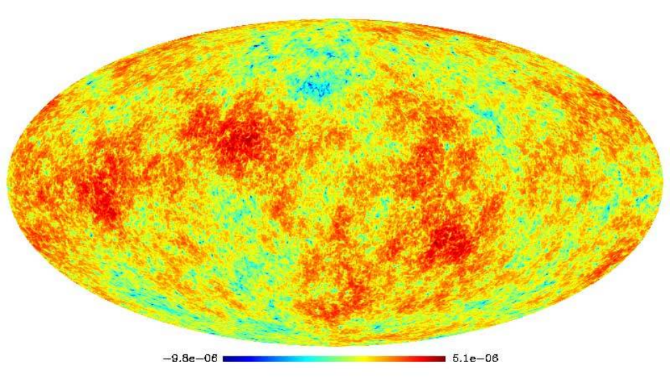

VI Direct comparison of bispectrum estimators
We have developed two complete numerical pipelines, implementing the eigenmode decomposition methods described in the previous sections. For a generic primordial shape or a given CMB bispectrum , an expansion in monomial symmetric polynomials is performed followed by the generation of nonGaussian map simulations. Bispectrum estimators are then applied to the map simulations in order to verify that the input can be properly recovered together with the expected variance. Both ‘early time decomposition’ and ‘late time decomposition’ estimators have been fully implemented. The former starts from an expansion of the primordial shape in Fourier space while the latter starts from an expansion of the reduced angular bispectrum in harmonic space, where in the second case radiation transfer functions have already been included in the expression for . The redundancy provided by the two alternative pipelines provide a further check of the reliability of the final results.
Since our purpose in this paper is to introduce the eigenmode expansion method, and to test its implementation, we will primarily apply our pipelines to map simulations, leaving detailed analysis of real datasets over a wider range of models for future publication [29]. As this is a proof-of-concept paper, we will mainly limit ourselves to the study of the simple equilateral family of models. This is because it is already well-studied in the literature (see e.g. [25, 31, 3]), which enables a useful comparison between the outcome of our numerical pipelines and previously published results for the equilateral shape. Moreover, the equilateral case does not require sophisticated noise analysis, unlike the local model. However, we will briefly consider other non-separable models outlined earlier in the introduction, such as the related DBI model and the cosmic string bispectrum. We note that from the point of view of the eigenmode decomposition, the formal separability of the equilateral shape is irrelevant; it does not cause early termination of the expansion series which is nearly identical to the non-separable DBI model (see fig. 10). Having established the reliability of the eigenmode expansion method here, in a forthcoming publication [29] we will apply it to the study of families of non-separable shapes using WMAP5 data.
VI.1 Simulated observational maps
Using the algorithm described in section V, we generated a set of equilateral CMB maps with both the primordial and late-time decomposition pipelines. We worked at roughly WMAP resolution with and HEALpix nside , corresponding to a pixel number . We then applied both our primordial and late-time estimators to both our primordial and late-time sets of simulated maps in all combinations. We found that in all cases the map-making methods gave consistent results, producing simulated maps from which the correct could be reliably recovered with the correct variance. Results for both primordial and late-time estimators on the same set of 50 equilateral maps (with and without the mask and inhomogeneous noise) with can be seen in fig. 15. We observe that the two estimators produce consistent results on the same maps. Of course, there is some small variation between the results as the two estimators can be regarded to be independent but this proved always to be well within the variance.
In addition, we extracted the equilateral configurations of the bispectrum from the maps and compared the average over all the simulations to the semi-analytic expectations obtained from the standard decomposition of the equilateral shape in terms of , , , (refer to eqns (25) and (28)). The recovered equilateral bispectrum values were in very good agreement between the semi-analytic prediction from the “standard” ,,, decomposition and the simulations, based on our eigenmode expansion, thus showing consistency with previous approaches.
Finally, we reiterate that this general approach to map simulation was highly efficient, producing Planck resolution maps for the equilateral model on short timescales. This made estimator validation through Monte Carlo simulatoins easily achievable with only modest resources. For other well-behaved bispectra, such as the cosmic string model, the general method proved robust. Examples of non-separable maps already have been discussed and shown in fig. 14.


VI.2 Primordial and late-time estimators
| Ideal simulations | WMAP5 simulations | |||
|---|---|---|---|---|
| Average | St. Dev. | Average | St. Dev. | |
| Primordial estimator | ||||
| Late-time estimator | ||||
| Internal st. dev. | ||||
Choosing an input value for the sets of equilateral map simulations described above, we compared results from both the primordial and late-time bispectrum estimators. In order to verify the consistency of the two methods we selected the late-time map sets and applied both estimators to it. The tests were performed starting from a noiseless full-sky map and then more realistic simulations were used, including partial sky-coverage and an anisotropic noise component. The rms noise was obtained by coadding WMAP V and W channel using the same scheme as the one adopted for nonGaussian analysis by the WMAP team [3]. The sky-coverage was done using the KQ75 mask, also adopted by the WMAP5 team for their analysis. Only the approximate form () of the estimator is used, and not the full form (II.3) including the full covariance matrix and a linear term. Note however that this approximation has been demonstrated in several previous studies to work well for equilateral shapes. Moreover, for our purposes the approximate nearly-optimal estimator is all we need since it contains all the dependence on the theoretical ansatz and thus all the dependence on our eigenmode expansion, which is the primary concern for this initial validation process.
We compared the recovered from each map using the two methods, as well as the final averages and variances. The variances were compared to expectations from Fisher matrix forecasts obtained both from our eigenmode expansion and from the ‘standard’ , , , decompostion of the equilateral shape used to date in other nonGaussian analysis. In all cases the results were internally consistent and in agreement with Fisher matrix expectations, as summarized in table (1). This led us to conclude that the eignemode expansion method appears to be a reliable way to produce non-Gaussian CMB simulations and estimators for primordial models, whether separable or otherwise.


Having verified the two estimator’s performance on simulated equilateral maps we then applied both of them to the WMAP5 data, coadding the V and W channels as discussed above. The primordial estimator obtained the result , which is consistent with the existing constraints obtained using standard separable primordial approach (given the caveat that a number of these results have now been superseded [10]). The constraint using the late-time estimator was which is slightly larger than the primordial result but still well within the range. As the late-time estimator can be regarded as independent of the primordial estimator, some variation is to be expected as we have seen already in fig. 15. The difference between the estimators is consistent with the internal variance of 103 noted in table 1 for equilateral map simulations in a WMAP-realistic context. We conclude that both the primordial and late-time estimators appear to be performing up to expectation.
Using the method described in eqn (117), we can endeavour to recover the full bispectrum from a given map. To illustrate this capability, we created a single map realization from an equilateral bispectra with , that is, a map with a nonGaussian signal. We then used the late-time estimator to recover the and mode coefficients described in (105). Recall that for results of sufficient significance, the should approximate the original theoretical model coefficients , that is, those used to generate the simulated map. We estimated the variance in each of the eigenmodes by applying the same method to 100 Gaussian simulations. The results for the orthornomal coefficients are plotted in fig. 16 for both ideal maps and for maps with inhomogeneous noise added and a mask applied. We see that we recover the first 7 modes well from the ideal map but the results from the map containing noise and mask are somewhat less encouraging. Clearly, more work is required to control noise and mask effects at higher mode numbers. By plotting the 3D bispectra from the reconstructions, see figure 17, we observe that it is possible to recover the main accoustic peak and some basic features of the CMB bispectra. We will address the challenging issues associated with bispectrum reconstruction in greater detail elsewhere [29].
VII Conclusions
We have now implemented two comprehensive and independent pipelines for the analysis and estimation of general primordial or CMB bispectra. Both methods are based on dual mode expansions, exploiting a complete orthonormal eigenmode basis to efficiently decompose arbitrary bispectra into a separable polynomial expansion. These separable mode expansions, whether at late or early times, allow a reduction of the computational overhead to easily tractable levels, whether calculating the reduced bispectrum , generating Planck resolution nonGaussian map simulations, or directly estimating from simulations or real data sets. The method exploits the smoothness of the pattern of acoustic peaks observed in calculations reviewing all well-behaved primordial models, implying the rapid convergence of the corresponding mode expansions. While most calculations are performed in the separable basis, a final rotation of mode coefficients into the orthonormal frame allows for a simple interpretation of the contributions to using Parseval’s theorem. In fact, the completeness of the orthonormal eigenmodes means, in principle, that it is straightforward to extract and reconstruct the full CMB bispectrum from the data, assuming the presence of a sufficiently significant nonGaussian signal.
The main purpose of this paper has been to present a detailed theoretical framework for estimation using separable eigenmode expansions, irrespective of the specific polynomials or other basis functions employed. However, we have also presented some numerical results from the pipelines we have implemented, chiefly for the equilateral model where there are extensive published results for direct comparison. An important milestone for the validation of this approach has been the development of a robust and reliable mode expansion method for generating map simulations from arbitrary bispectra. While generalising previous methods applied to specific separable cases, we noted that the scale-invariance of the polynomial expansion modes eliminates numerical instabilities that previously had to be circumvented on a case-by-case basis. Given convergent mode expansions for well-behaved bispectra, high resolution map simulations for a wide variety of models can easily and efficiently be generated, with several examples illustrated here including late-time cosmic strings. The many map simulations created for the equilateral model with both primordial and late-time methods showed consistency in expected variance and recovery.
The primordial and late-time estimators using mode expansions were tested successfully on the simulated equilateral maps, matching expectations for semi-analytic Fisher matrix forecasts and providing consistent unbiased results for . This was achieved for both ideal maps and in a WMAP-realistic context, incorporating beams, anisotropic noise and a mask. Application of the estimators to the WMAP5 data gave constraints on the equilateral model consistent with each other and previously published results. These encouraging results suggest that the approach will provide a robust and general framework for estimation for the wide variety of non-separable models which remain to be constrained [11]. For single equilateral map simulation with , we were able to demonstrate a reasonable correspondence between the theoretical and recovered mode expansion coefficients, while also being able to recover key features of the full CMB bispectrum. However, a detailed discussion of such prospects has been left for a future publication [29]. We have also left aside for discussion elsewhere a more sophisticated treatment of sky cuts and inhomogeneous noise, which is more important for the analysis of the local model, as well as the potential for incorporating polarisation data. Challenges remain for the full implementation of the primordial and late-time pipelines at Planck resolution, but the generality and robustness of this methodology suggests that it should prove to be a useful tool for exploring and constraining a much wider class of nonGaussian models.
VIII Acknowledgements
We are very grateful for informative discussions with Xingang Chen and Kendrick Smith and we have also benefitted from useful conversations with Martin Bucher, Anthony Challinor, Olivier Forni, Enrique Martinez-Gonzalez and Bartjan van Tent. The ongoing development of these methods has been regularly reported at Planck Working Group 4 (NonGaussianity), where we have been grateful for feedback and to learn of related work. Simulations were performed on the COSMOS supercomputer (an Altix 4700) which is funded by STFC, HEFCE and SGI. JRF, ML and EPS were supported by STFC grant ST/F002998/1 and the Centre for Theoretical Cosmology.
References
- [1] Juan Martin Maldacena. Non-Gaussian features of primordial fluctuations in single field inflationary models. JHEP, 05:013, 2003.
- [2] Viviana Acquaviva, Nicola Bartolo, Sabino Matarrese, and Antonio Riotto. Second-order cosmological perturbations from inflation. Nucl. Phys., B667:119–148, 2003.
- [3] E. Komatsu et al. Five-Year Wilkinson Microwave Anisotropy Probe (WMAP) Observations:Cosmological Interpretation. Astrophys. J. Suppl., 180:330–376, 2009.
- [4] Amit P. S. Yadav and Benjamin D. Wandelt. Evidence of Primordial Non-Gaussianity in the Wilkinson Microwave Anisotropy Probe 3-Year Data at 2.8. Phys. Rev. Lett., 100:181301, 2008.
- [5] A. Curto et al. WMAP 5-year constraints on fnl with wavelets. 2008.
- [6] Oystein Rudjord et al. An Estimate of the Primordial Non-Gaussianity Parameter Using the Needlet Bispectrum from WMAP. Astrophys. J., 701:369–376, 2009.
- [7] Kendrick M. Smith, Leonardo Senatore, and Matias Zaldarriaga. Optimal limits on from WMAP 5-year data. JCAP, 0909:006, 2009.
- [8] ESA Planck Consortium. Planck: The Scientific Programme (Planck Blue Book). 2005.
- [9] Eiichiro Komatsu, David N. Spergel, and Benjamin D. Wandelt. Measuring primordial non-Gaussianity in the cosmic microwave background. Astrophys. J., 634:14–19, 2005.
- [10] Leonardo Senatore, Kendrick M. Smith, and Matias Zaldarriaga. Non-Gaussianities in Single Field Inflation and their Optimal Limits from the WMAP 5-year Data. 2009.
- [11] J. R. Fergusson and E. P. S. Shellard. The shape of primordial non-Gaussianity and the CMB bispectrum. Phys. Rev., D80:043510, 2009.
- [12] Mark Hindmarsh, Christophe Ringeval, and Teruaki Suyama. The CMB temperature bispectrum induced by cosmic strings. Phys. Rev., D80:083501, 2009.
- [13] D. M. Regan and E. P. S. Shellard. Cosmic String Power Spectrum, Bispectrum and Trispectrum. 2009.
- [14] J. R. Fergusson and Edward P. S. Shellard. Primordial non-Gaussianity and the CMB bispectrum. Phys. Rev., D76:083523, 2007.
- [15] Emiliano Sefusatti, Michele Liguori, Amit P. S. Yadav, Mark G. Jackson, and Enrico Pajer. Constraining Running Non-Gaussianity. 2009.
- [16] A. Curto, E. Martinez-Gonzalez, and R. B. Barreiro. Improved constraints on primordial non-Gaussianity for the Wilkinson Microwave Anisotropy Probe 5-yr data. Astrophys. J., 706:399–403, 2009.
- [17] Martin Bucher, Bartjan Van Tent, and Carla Sofia Carvalho. Detecting Bispectral Acoustic Oscillations from Inflation Using a New Flexible Estimator. 2009.
- [18] Daniel Babich, Paolo Creminelli, and Matias Zaldarriaga. The shape of non-Gaussianities. JCAP, 0408:009, 2004.
- [19] G. I. Rigopoulos, E. P. S. Shellard, and B. J. W. van Tent. Large non-Gaussianity in multiple-field inflation. Phys. Rev., D73:083522, 2006.
- [20] Xingang Chen and Yi Wang. Large non-Gaussianities with Intermediate Shapes from Quasi-Single Field Inflation. 2009.
- [21] Paolo Creminelli. On non-gaussianities in single-field inflation. JCAP, 0310:003, 2003.
- [22] Mohsen Alishahiha, Eva Silverstein, and David Tong. DBI in the sky. Phys. Rev., D70:123505, 2004.
- [23] Xingang Chen, Min-xin Huang, Shamit Kachru, and Gary Shiu. Observational signatures and non-Gaussianities of general single field inflation. JCAP, 0701:002, 2007.
- [24] Daniel Babich. Optimal Estimation of Non-Gaussianity. Phys. Rev., D72:043003, 2005.
- [25] Paolo Creminelli, Alberto Nicolis, Leonardo Senatore, Max Tegmark, and Matias Zaldarriaga. Limits on non-Gaussianities from WMAP data. JCAP, 0605:004, 2006.
- [26] Amit P. S. Yadav et al. Fast Estimator of Primordial Non-Gaussianity from Temperature and Polarization Anisotropies in the Cosmic Microwave Background II: Partial Sky Coverage and Inhomogeneous Noise. Astrophys. J., 678:578, 2008.
- [27] E. Komatsu et al. Five-Year Wilkinson Microwave Anisotropy Probe (WMAP) Observations:Cosmological Interpretation. 2008.
- [28] Huiyuan Li and Yuan Xu. Discrete Fourier analysis on a dodecahedron and a tetrahedron. 2008.
- [29] James R. Fergusson, Michele Liguori, and Edward P. S. Shellard. CMB constraints on non-Gaussianity, in preparation. 2009.
- [30] Ian G Moss and Chun Xiong. Non-gaussianity in fluctuations from warm inflation. JCAP, 0704:007, 2007.
- [31] Kendrick M. Smith and Matias Zaldarriaga. Algorithms for bispectra: forecasting, optimal analysis, and simulation. ArXiv Astrophysics e-prints, 2006.
- [32] Duncan Hanson, Kendrick M. Smith, Anthony Challinor, and Michele Liguori. CMB lensing and primordial non-Gaussianity. Phys. Rev., D80:083004, 2009.