Cosmological data analysis of gravity models
Abstract:
A class of well-behaved modified gravity models with long enough matter domination epoch and a late-time accelerated expansion is confronted with SNIa, CMB, SDSS, BAO and galaxy ages data, as well as current measurements of the linear growth of structure. We show that the combination of geometrical probes and growth data exploited here allows to rule out gravity models, in particular, the logarithmic of curvature model. We also apply solar system tests to the models in agreement with the cosmological data. We find that the exponential of the inverse of the curvature model satisfies all the observational tests considered and we derive the allowed range of parameters. Current data still allows for small deviations of Einstein gravity. Future, high precision growth data, in combination with expansion history data, will be able to distinguish tiny modifications of standard gravity from the CDM model.
Keywords:
Modified Gravity, Linear perturbation theory1 Introduction
Astronomical observations have led to the inference that our universe is approximately flat and its mass-energy budget consists of ordinary matter, non-baryonic dark matter, plus a dominant negative-pressure component that accelerates the Hubble expansion [1, 2, 3, 4, 5]. The current accelerated expansion of the universe reveals new physics missing from our universe’s picture, and it constitutes the fundamental key to understand the fate of the universe.
The most economical description of the cosmological parameters attributes the negative-pressure dark energy component to a cosmological constant (CC) in Einstein’s equations. The CC represents an invariable vacuum energy density that assumes a greater importance as the Universe expands. The equation of state of the dark energy component in the CC case is constant and , where and denote dark energy pressure and energy density, respectively. However, when computing the vacuum energy density from the quantum field theory approach, the naively expected value exceeds the measured one by 123 orders of magnitude and it needs to be cancelled by extreme fine-tuning. This is the so-called CC problem. A related problem is the so called why now? or coincidence problem, i.e. why the dark matter and dark energy contributions to the energy budget of the universe are similar at this precise moment of the cosmic history.
A dynamical alternative attributes the accelerated expansion to a cosmic scalar field, quintessence [6, 7, 8, 9, 10, 11], that changes with time and varies across space, slowly approaching its ground state. In this case, the equation of state could vary over time. However, quintessence models are not better than the CC scenario as regards fine-tuning, since there is no symmetry that explains the tiny value of the potential at its ground state.
There exists another possible scenario, in which the gravitational sector is modified, as an alternative to explain the observed cosmic acceleration. Although this requires the modification of Einstein’s equations of gravity on very large distances [12], or on small curvatures [13, 14, 15], this is not unexpected for an effective 4-dimensional description of higher dimensional theories. Modifications of gravity have been examined in the context of accelerated expansion. The proposed modified gravity models have extra spatial dimensions or an action which is non linear in the curvature scalar, that is, these models include extensions of the Einstein-Hilbert action, for instance, to higher derivative theories [16], scalar-tensor theories or generalized functions of the Ricci scalar .
Among a plethora of models, a recent study [17] has identified those cosmologically acceptable, i.e. models with a standard matter era followed by an accelerated attractor. We focus here on the cosmological bounds on these viable models. We use recent SNIa, BAO, CMB and galaxy ages data to constrain the background evolution in this class of models. We exploit as well current measurements of the linear growth of structure, which provides us an additional test to be combined with the background probes. The models which are not ruled out by the global cosmological analysis will be examined under solar system constraints.
The structure of the paper is as follows. We start in Sec. 2 specifying the class of modified gravity models explored here, as well as the equations which describe the background evolution and the linear perturbation theory in a generic model. Section 3 contains a description of the different cosmological data sets used in the analysis performed here. Our results are presented in Sec. 4. We describe the solar system constraints in Sec. 5. We summarize our results, draw our conclusions and discuss future work in Sec. 6.
2 Models
We investigate the simplest family of modified gravity models, obtained by adding to the usual Hilbert-Einstein Lagrangian some function of the Ricci scalar , with an action given by
| (1) |
Here we analyse models which are cosmologically viable, i.e., models which predict a matter dominated period followed later by an accelerated expansion epoch. In the matter domination era the effective equation of state is close to and the scale factor grows with time as .
The authors of [17] have explored the general conditions for the cosmological viability of models in the context of a flat, homogeneous and isotropic background. The cosmological behaviour of models can be characterized by studying the curve on the plane [17], where
| (2) |
and . A given model will have a standard matter dominated period followed by a late time accelerated era if the conditions and at are satisfied, respectively.
Reference [17] shows that all models with an
accelerated global attractor belong to four classes,
two of which can be cosmologically acceptable: models of Class II,
asymptotically equivalent to the
CDM model (), and models of Class IV,
which have a non-phantom final accelerated expansion period
(). In practice, there are not models belonging
to Class IV, unless they are built by hand from a well-behaved function.
There are other type of models, as those from Class III,
which have an unstable matter era followed by
a phantom acceleration (). These Class III
models are generally ruled out by observations, although a more
careful numerical analysis is needed.
We focus here on the Class II models of Ref. [17], studying the following four cases:
| (3) | |||||
| (4) | |||||
| (5) | |||||
| (6) |
2.1 Background evolution
The field equations, which can be obtained varying the action (1) with respect to , read
| (7) |
The metric we take is of the form of a flat Friedman Robertson Walker (FRW) background , with the scale factor. The Friedmann equation is given by
| (8) |
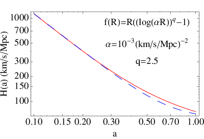
where , denotes the Hubble expansion rate , refers to the total cold dark matter energy density and . The present dark matter energy density has been fixed to (when not treated as a free parameter), accordingly to a recent fit to cosmological data [2]. We have integrated numerically the background equation (8) for the four Class II functions given by Eqs. (3), (4), (5) and (6). We have determined the ranges of the free parameters which lead to a value of the Hubble constant within its current 1 range km/s/Mpc [18]. Figure I shows the results for the Hubble parameter for the four different models explored here. As a comparison, we depict as well the Hubble rate for a flat universe with a CC (CDM model)** * The Hubble rate for the CDM model, neglecting the radiation contribution, reads .. The values for the choice of parameters used in Fig. I are and km/s/Mpc for , , and , respectively.
 |
 |
 |
 |
2.2 Linear growth rate
We consider scalar linear perturbations around a flat FRW background in the Newtonian gauge
| (9) |
The perturbations to the metric are the Newtonian potential and the perturbation to the spatial curvature . Since we are working in the Jordan frame, in which matter is minimally coupled, the conservation equations for the cold dark matter component have the same form than in general relativity. At first order in the perturbations, the conservation equations read
| (10) |
where means derivative with respect to , is the cold dark matter overdensity and is the dark matter (comoving) peculiar velocity divergence. For subhorizon modes (), and in the quasi-static limit†† † In this limit time derivatives are assumed to be negligible with respect to spatial derivatives., the perturbed and () components of the Einstein equations read
| (11) | |||||
| (12) |
where we have set the anisotropic stress of cold dark matter to zero, refers to the cold dark matter energy density and we have neglected the radiation contribution. The factor is defined as
| (13) |
By substituting the equation for the component into the one for the component one gets the modified Poisson equation
| (14) |
which reduces to the standard one if . The growth factor equation is obtained by combining Eqs. (10) and Eq. (14), see also Ref. [19]:
| (15) |
where , and is normalized such that
when . In general relativity, the
factor given by Eq. (13) is zero and therefore the linear
density growth is scale independent for all dark energy
models. However, for models, the scale dependent
induces a nontrivial scale dependence of the growth .
We illustrate this scale dependence of the growth factor in
Fig. II, where it is shown the present value of the
matter overdensity as a
function of the scale for the four models considered
here. We depict as well the current value of the matter
overdensity for a CDM universe. Notice that, for the choice of
parameters which ensure an acceptable ,
the growth of matter perturbations within the
model is highly suppressed with
respect to the growth in a universe with a CC.
For the other three models the growth is very close to the
CDM growth at large scales. However, it shows a dependence as increases, due to a larger factor, see Eq. (13).
Galaxy surveys provide information on , where is the logarithmic
derivative of the linear growth rate, i.e. . Therefore for our numerical
analyses we will use , see the details
in the next section.
 |
 |
 |
 |
3 Cosmological data used in the analysis
In this section we describe the cosmological data used in our numerical analyses‡‡ ‡ For practical purposes, in the following, we will use the redshift instead of the scale factor .. Four different geometrical probes (SNIa, CMB, BAO and galaxy ages datasets) will be combined with growth of structure data to derive the cosmological bounds on the free parameters of the models explored here, see Eqs. (3), (4), (5) and (6).
3.1 The Supernova Union Compilation
The Union Compilation [3] is a collection of 414 SNIa, which reduces to 307 SNe after selection cuts. It includes the recent large samples of SNIa from the Supernova Legacy Survey and ESSENCE Survey, and the recently extended dataset of distant supernovae observed with the Hubble Space Telescope (HST). In total the Union Compilation presents 307 values of distance moduli (), with relative errors, ranging from a redshift of 0.05 up to . The distance moduli, i.e. the difference between apparent and absolute magnitude of the objects, is given by
| (16) |
where is the luminosity distance, . The function used in the analysis reads
| (17) |
where, here and in the following, will refer to the free parameters of the f(R) models.
3.2 CMB first acoustic peak
We use here the CMB shift parameter , since it is the least model dependent quantity extracted from the CMB power spectrum [20], i.e. it does not depend on the present vale of the Hubble parameter . The reduced distance is written as
| (18) |
The WMAP-5 year CMB data alone yields for a fit assuming a constant [2]. The is defined as .
3.3 BAOs
An independent geometrical probe are BAO measurements. Acoustic oscillations in the photon-baryon plasma are imprinted in the matter distribution. These BAOs have been detected in the spatial distribution of galaxies by the SDSS [21] at a redshift and the 2dF Galaxy Reshift Survey [22] at a redshift . The oscillation pattern is characterized by a standard ruler, , whose length is the distance sound can travel between the Big Bang and recombination and at which the correlation function of dark matter (and that of galaxies, clusters) should show a peak. While future BAO data is expected to provide independent measurements of the Hubble rate and of the angular diameter distance at different redshifts, current BAO data does not allow to measure them separately, so they use the spherically correlated function
| (19) |
In Ref. [23], a tension among SDSS abd BAO datasets was claimed. Therefore, we will focus on the SDSS dataset in the following. The SDSS team reports its BAO measurements in terms of the parameter,
| (20) |
where . The function is defined as .
3.4 Galaxy ages
We use the data extracted from galaxy ages in the redshift range , see Ref. [24]. The authors first selected galaxy samples of passively evolving galaxies with high-quality spectroscopy. Second, they used synthetic stellar population models to constrain the age of the oldest stars in the galaxy (after marginalising over the metallicity and star formation history) and then computed differential ages and used them as their estimator for , which in turn gave . We use the eight data points shown in Figure 1 in Ref. [24] to test cosmological models by these data sample. The function is defined as
| (21) |
3.5 Growth factor
Galaxy surveys measure the redshift of the galaxies, providing, therefore, the redshift space galaxy distributions. From those redshifts the radial position of the galaxy is extracted. However, the inferred galaxy distribution (and, consequently, the power spectrum) is distorted with respect to the true galaxy distribution, because in redshift space one neglects the peculiar velocities of the galaxies. These are the so called redshift space distortions.
In linear theory and with a local linear galaxy bias the relation between the true spectrum in real space and the spectrum in redshift space reads
| (22) |
where , being the logarithmic derivative of the growth factor, and is the cosine of the angle between the line of sight and the wavevector . Notice that perturbations with perpendicular to the line of sight are not distorted. By averaging over all directions , one obtains the relation
| (23) |
The relation among real space and redshift space overdensities given by Eq. (22) was first derived by Kaiser [25] and it arises from the continuity equation, which relates the divergence of the peculiar velocity with the linear matter overdensity. Redshift space distortions, then, relate peculiar velocities with the growth factor . A measurement of will provide information on the growth of structure formation if the galaxy bias is known. One can estimate the redshift distortion parameter both by using the ratio of the redshift space correlation function to the real space correlation function, see Eq. (23) and by exploiting the ratio of the monopole and quadrupole harmonics of the redshift correlation function [26]:
| (24) |
We quote the current available data on , the galaxy bias and the inferred growth factor in Tab. 1. Notice from the first of Eqs. (10) that the continuity equation in theories is exactly the same than in general relativity and therefore the relation between peculiar velocities and the matter overdensity is not modified in the models studied here. Consequently, we use the available data on the logarithmic derivative of the growth factor , see Tab. 1 as an additional test for models, to be added to the geometrical probes previously described. The function is defined as . Notice that the theoretical prediction for the growth factor is scale dependent. We choose Mpc-1 to be within the linear regime and within the scale range tested by current surveys, see Tab. 1.
4 Analysis of cosmological models
In this section we present the constraints in four modified gravity models (see Eqs. (3) to (6)) which arise from the datasets described in the previous section. These models have been shown to have a long enough matter domination epoch and late-time accelerated expansion [17].
We show below that the combination of geometrical probes (i.e. distance measurements) and growth of structure data allows to exclude some models. For those consistent with all the cosmological data sets used here, we derive the allowed range of parameters and discuss the near future improvements. We will see in next section that some of the models consistent with all cosmological data, are excluded by solar system tests.
In the discussion, we make use of the individual chi-square functions, the global chi-square defined by
and the only-distances , defined as the global chi-square without the last term. If not otherwise specified, the cosmological parameters and are fixed to the values Km/s/Mpc and respectively.
4.1 Model H1: (, )
This model contains two parameters: the power index of the curvature and the normalization of the modification of gravity . The model contains the CDM universe as a limiting case: if , then , where the parameter becomes a cosmological constant. Therefore, it must be allowed by the cosmological data within a parameter range. The best fit model is acceptable for all the independent data sets and the full data analysis gives a of 325.3 for 322 d.o.f..
We firstly discuss the larger allowed, and how much deviates from the cosmological constant present in a CDM universe. In Fig. III we show the , and CL contours (full colour) resulting from a fit to all the cosmological data exploited here. The global best fit point is marked by a star. Notice that the power index can be quite large and that the normalization can depart from the cosmological constant value. In fact, data prefer and (km/s/Mpc)2×(1-0.11), far from the cosmological constant () limiting case ( (km/s/Mpc)2 and ).
The regions allowed by growth of structure data are depicted by dashed lines, with the best fit point marked as a plus sign. The allowed regions from a fit to distance measurements (i.e. geometrical probes) are depicted by black lines. The statistical power is dominated by distance data: only an expert eye can notice the difference among the global analysis allowed regions and those coming from the only-distances analysis. SNIa data are the most important piece of information that constrains the modified gravity parameters. BAO, CMB and galaxy ages data sets have a similar weight in the statistical analysis.
Figure III shows some tension between the model predictions and the different data sets for the largest allowed values of . Notice that additional, high precision growth data may further test the high region and further constrain the deviations of the model from a CDM universe.

4.2 Model H2: ()
This model is described by two parameters: the power index of the logarithm of the curvature and a normalization of the modification of gravity . The best fit model is acceptable for the all the distance measurements, with some tension between the allowed ranges derived from the different distance observables.
The relevance of testing this model against cosmological data appears when we compare the allowed regions by geometrical probes to those coming from a fit to growth of structure data: there is no allowed region at more than 99.73% CL able to fit distances and growth data simultaneously, see Fig. IV.
Distance measurements prefer larger values of the power index , while growth data prefer a much smaller power index. Notice that for parameters that reproduce correctly the expansion history, the linear growth is k-independent but very much off the CDM model (see Figs. I and II). Errors in the inferred growth rate are still large (see Tab. 1), but sufficient to test this model. We obtain for 322 d.o.f., with a probability of the result being due to chance . Statistically, we can reject the null hypothesis of the model being compatible with data.

4.3 Model H3:
This model contains one free parameter . We also allow here the current fraction of the energy density in the form of dark matter, , to be an additional free parameter.
The model contains the cosmological constant model as a limiting case. If is small, then , where the parameter becomes a cosmological constant. The best fit model is acceptable for all the independent data sets and the full data analysis gives a of 332.4 for 322 d.o.f..
Figure V depicts the , and CL contours (full colour) resulting from a fit to all the cosmological data exploited here. The parameter can deviate from the cosmological constant in CDM by less than 10%. From the global analysis we obtain and (km/s/Mpc)2. The distances only data mostly contributes to strongly constrain the parameter of this modified gravity model. Notice from Fig. V that the growth data prefer smaller values of and , pushing down the global allowed region respect to the distances only allowed region. Not surprisingly, the best fit of the analysis lies outside the region shown here. Future more accurate growth of structure data could provide tighter bounds on the parameters and , and potentially reject this model if it would not fit simultaneously distances and future growth data.

4.4 Model H4: ()
The () model is described by two parameters: the cosmological constant and the normalization of the modification of gravity . If , then , a cosmological constant, implying that the model must work in some parameter range. Notice that the Einstein Hilbert action contains the term , and therefore the is twice the usual cosmological constant . The best fit model is acceptable for all the independent data sets and the full data analysis gives a of 323.6 for 322 d.o.f..
Figure VI depicts the , and CL contours (full colour) resulting from a fit to all the cosmological data exploited here. The data prefer a very small modification of gravity with . The best fit point of the global analysis is and (km/s/Mpc)2, which is about 1- away from the preferred without a modification of gravity (i.e. ). High precision future geometrical probes can reduce the model to a negligible perturbation of the CDM model.

5 Solar system constraints
We explore here the weak field limit of , and , modified gravity models which have been shown to be consistent with the cosmological probes used in the previous section.
It is well known that gravity models that produced late time acceleration also have problems to pass solar system tests [32, 33, 34, 35, 36, 37, 38, 39, 40, 41, 42]. The reason is that gravity theories introduce a scalar degree of freedom given by that, for the background cosmological density, is very light. As a consequence, it produces a long-range fifth force, leading to a dissociation of the space-time curvature from the local density. Then, the metric around the sun is predicted to be different than what is observed. Chiba [43] has shown under which conditions an gravity is equivalent to a scalar-tensor theory with Parametrized Post-Newtonian (PPN) parameter , far outside the range allowed by observations, [44].
However, some theories are still viable: the scalar field mass could be large and therefore it would not have an effect at solar system scales. Another possibility is a scale dependent scalar field mass, as in the chameleon mechanism [45, 46, 47, 48, 49]. In chameleon cosmologies, the effective mass of the scalar field becomes very large in high density environments (as in the Sun’s interior) and the induced fifth force range would be below the detectability level of gravitational experiments.
In what follows we will apply the criteria presented by Hu and Sawicki in Ref. [38]. If the system’s density (for instance, the Sun’s density) changes on scales that are much larger than the scalar field Compton wavelength
| (25) |
where
| (26) |
the curvature will follow the Sun’s density, as in general relativity. This is the Compton condition. If it is satisfied at all radii, high densities will be associated with high curvature and deviations from general relativity will be highly suppressed. If the Compton condition is not satisfied, one would need then to check the thin-shell condition. This condition applies when the (massive) scalar field is trapped within the system and its influence is only due to a thin shell, shielding the fifth force mediated by the scalar field. For the solar system, the thin shell criterion reads [47, 38]
| (27) |
where is the field difference from far inside the body to very far away. Local gravity constraints for the model H1, have been already studied in [40], where it is found that only is allowed. Such values of are too close to CDM, and therefore not interesting cosmologically.
We find that the only model which satisfies the Compton condition and therefore satisfies solar system constraints is . The Compton wavelength for this model is . For the best fit values of (km/s/Mpc)2 and for densities corresponding to the solar corona g/cm3, . For higher densities, the Compton wavelength is even smaller and therefore the curvature will follow the density profile inside the Sun, as in general relativity.
The other two models which survive the cosmological , i.e. and do not satisfy the Compton nor the thin shell criteria, and therefore they are ruled out by solar system observations.
6 Discussion
We have studied a class of modified gravity models, which possess a long enough matter domination epoch and late-time accelerated expansion, as identified by the authors of [17]. Both the background evolution and the growth of structure have been computed in these well behaved modified gravity cosmologies. We have confronted the expansion history in these cosmologies with SNIa data, the CMB shift parameter , the SDSS BAO measurement and the data derived from galaxy ages. We have also fitted the linear growth of structure in these models to the growth information derived from redshift space distortions, as a novel approach.
Interestingly, we find that the cosmological data exploited here possess an enormous potential to rule out modified gravity models. models with a good expansion history like badly fail to reproduce the growth measurements and can be statistically rejected with present data.
Other modified gravity models as , and are allowed by all the cosmological data exploited in this study, and include as a limiting case a CDM universe. We show the allowed range of parameters in these models, finding that modifications of gravity must be small. The bounds presented here could be greatly improved with future high precision growth data.
We have also studied the solar system bounds on the three models which agree with the cosmological data. The only model which satisfies solar system constraints is . The other two models, although cosmologically viable, are ruled out by solar system observations.
From a global fit (which includes SNIa, CMB, BAO, galaxy ages and growth data) to the parameter in the exponential model and to the current matter energy density , we obtain and (km/s/Mpc)2. Geometrical probes mostly contribute to strongly constrain the parameter of this modified gravity model, while growth data slightly prefer lower values of both parameters and . In the parameter allowed region where the exponential model differs from the standard CC cosmology, we find that the growth factor is -dependent, in contrast to the CDM prediction. More precise growth data at small scales, albeit still within the linear regime, will potentially find small deviations from a universe with a CC.
Our study shows, with the exploration of several models, that the combination of geometrical probes and growth data offers a powerful tool to rule out modified gravity scenarios and/or constrain deviations from the CDM picture. We can anticipate that future growth of structure data in the linear regime, combined with a full analysis including the nonlinear regime, will have a very important impact in searching for tiny deviations from Einstein gravity.
Acknowledgments
O.M. and N.R. thank the Fermilab theory group for hospitality. This work is supported in part by the Spanish MICINN grants FPA-2007-60323 and AYA2008-03531, the Consolider Ingenio-2010 project CSD2007-00060 and the Generalitat Valenciana grant PROMETEO/2009/116. The work of O.M. is supported by a Ramón y Cajal contract.
References
- [1] WMAP Collaboration, J. Dunkley et. al., Five-Year Wilkinson Microwave Anisotropy Probe (WMAP) Observations: Likelihoods and Parameters from the WMAP data, Astrophys. J. Suppl. 180 (2009) 306–329, [arXiv:0803.0586].
- [2] WMAP Collaboration, E. Komatsu et. al., Five-Year Wilkinson Microwave Anisotropy Probe (WMAP) Observations:Cosmological Interpretation, Astrophys. J. Suppl. 180 (2009) 330–376, [arXiv:0803.0547].
- [3] M. Kowalski et. al., Improved Cosmological Constraints from New, Old and Combined Supernova Datasets, Astrophys. J. 686 (2008) 749–778, [arXiv:0804.4142].
- [4] SDSS Collaboration, M. Tegmark et. al., Cosmological Constraints from the SDSS Luminous Red Galaxies, Phys. Rev. D74 (2006) 123507, [astro-ph/0608632].
- [5] W. J. Percival et. al., The shape of the SDSS DR5 galaxy power spectrum, Astrophys. J. 657 (2007) 645–663, [astro-ph/0608636].
- [6] R. R. Caldwell, R. Dave, and P. J. Steinhardt, Quintessential cosmology: Novel models of cosmological structure formation, Astrophys. Space Sci. 261 (1998) 303–310.
- [7] I. Zlatev, L.-M. Wang, and P. J. Steinhardt, Quintessence, Cosmic Coincidence, and the Cosmological Constant, Phys. Rev. Lett. 82 (1999) 896–899, [astro-ph/9807002].
- [8] L.-M. Wang, R. R. Caldwell, J. P. Ostriker, and P. J. Steinhardt, Cosmic Concordance and Quintessence, Astrophys. J. 530 (2000) 17–35, [astro-ph/9901388].
- [9] C. Wetterich, The Cosmon model for an asymptotically vanishing time dependent cosmological ’constant’, Astron. Astrophys. 301 (1995) 321–328, [hep-th/9408025].
- [10] P. J. E. Peebles and B. Ratra, Cosmology with a Time Variable Cosmological Constant, Astrophys. J. 325 (1988) L17.
- [11] B. Ratra and P. J. E. Peebles, Cosmological Consequences of a Rolling Homogeneous Scalar Field, Phys. Rev. D37 (1988) 3406.
- [12] G. R. Dvali, G. Gabadadze, and M. Porrati, 4D gravity on a brane in 5D Minkowski space, Phys. Lett. B485 (2000) 208–214, [hep-th/0005016].
- [13] S. M. Carroll, V. Duvvuri, M. Trodden, and M. S. Turner, Is cosmic speed-up due to new gravitational physics?, Phys. Rev. D70 (2004) 043528, [astro-ph/0306438].
- [14] S. Capozziello, S. Carloni, and A. Troisi, Quintessence without scalar fields, Recent Res. Dev. Astron. Astrophys. 1 (2003) 625, [astro-ph/0303041].
- [15] D. N. Vollick, Curvature Corrections as the Source of the Cosmological Acceleration, Phys. Rev. D68 (2003) 063510, [astro-ph/0306630].
- [16] S. M. Carroll et. al., The cosmology of generalized modified gravity models, Phys. Rev. D71 (2005) 063513, [astro-ph/0410031].
- [17] L. Amendola, R. Gannouji, D. Polarski, and S. Tsujikawa, Conditions for the cosmological viability of f(R) dark energy models, Phys. Rev. D75 (2007) 083504, [gr-qc/0612180].
- [18] A. G. Riess et. al., A Redetermination of the Hubble Constant with the Hubble Space Telescope from a Differential Distance Ladder, Astrophys. J. 699 (2009) 539–563, [arXiv:0905.0695].
- [19] R. Bean, D. Bernat, L. Pogosian, A. Silvestri, and M. Trodden, Dynamics of Linear Perturbations in f(R) Gravity, Phys. Rev. D75 (2007) 064020, [astro-ph/0611321].
- [20] Y. Wang and P. Mukherjee, Robust Dark Energy Constraints from Supernovae, Galaxy Clustering, and Three-Year Wilkinson Microwave Anisotropy Probe Observations, Astrophys. J. 650 (2006) 1, [astro-ph/0604051].
- [21] SDSS Collaboration, D. J. Eisenstein et. al., Detection of the Baryon Acoustic Peak in the Large-Scale Correlation Function of SDSS Luminous Red Galaxies, Astrophys. J. 633 (2005) 560–574, [astro-ph/0501171].
- [22] W. J. Percival et. al., Measuring the Baryon Acoustic Oscillation scale using the SDSS and 2dFGRS, Mon. Not. Roy. Astron. Soc. 381 (2007) 1053–1066, [arXiv:0705.3323].
- [23] A. G. Sanchez and S. Cole, The galaxy power spectrum: precision cosmology from large scale structure?, Mon. Not. Roy. Astron. Soc. 385 (2008) 830–840, [arXiv:0708.1517].
- [24] J. Simon, L. Verde, and R. Jimenez, Constraints on the redshift dependence of the dark energy potential, Phys. Rev. D71 (2005) 123001, [astro-ph/0412269].
- [25] N. Kaiser, Clustering in real space and in redshift space, Mon. Not. Roy. Astron. Soc. 227 (1987) 1–27.
- [26] A. J. S. Hamilton, Measuring Omega and the real correlation function from the redshift correlation function, Astrophys. J. 385 (Jan., 1992) L5–L8.
- [27] L. Verde et. al., The 2dF Galaxy Redshift Survey: The bias of galaxies and the density of the Universe, Mon. Not. Roy. Astron. Soc. 335 (2002) 432, [astro-ph/0112161].
- [28] E. Hawkins et. al., The 2dF Galaxy Redshift Survey: correlation functions, peculiar velocities and the matter density of the Universe, Mon. Not. Roy. Astron. Soc. 346 (2003) 78, [astro-ph/0212375].
- [29] N. P. Ross et. al., The 2dF-SDSS LRG and QSO Survey: The 2-Point Correlation Function and Redshift-Space Distortions, astro-ph/0612400.
- [30] L. Guzzo et. al., A test of the nature of cosmic acceleration using galaxy redshift distortions, Nature 451 (2008) 541–545, [arXiv:0802.1944].
- [31] S. Nesseris and L. Perivolaropoulos, Testing LCDM with the Growth Function : Current Constraints, Phys. Rev. D77 (2008) 023504, [arXiv:0710.1092].
- [32] T. Chiba, 1/R gravity and scalar-tensor gravity, Phys. Lett. B575 (2003) 1–3, [astro-ph/0307338].
- [33] I. Navarro and K. Van Acoleyen, On the Newtonian limit of Generalized Modified Gravity Models, Phys. Lett. B622 (2005) 1–5, [gr-qc/0506096].
- [34] G. J. Olmo, Post-Newtonian constraints on cosmologies in metric and Palatini formalism, Phys. Rev. D72 (2005) 083505.
- [35] G. J. Olmo, The gravity lagrangian according to solar system experiments, Phys. Rev. Lett. 95 (2005) 261102, [gr-qc/0505101].
- [36] S. Capozziello and A. Troisi, PPN-limit of fourth order gravity inspired by scalar- tensor gravity, Phys. Rev. D72 (2005) 044022, [astro-ph/0507545].
- [37] I. Navarro and K. Van Acoleyen, f(R) actions, cosmic acceleration and local tests of gravity, JCAP 0702 (2007) 022, [gr-qc/0611127].
- [38] W. Hu and I. Sawicki, Models of f(R) Cosmic Acceleration that Evade Solar-System Tests, Phys. Rev. D76 (2007) 064004, [arXiv:0705.1158].
- [39] G. J. Olmo, Limit to general relativity in f(R) theories of gravity, Phys. Rev. D75 (2007) 023511, [gr-qc/0612047].
- [40] L. Amendola and S. Tsujikawa, Phantom crossing, equation-of-state singularities, and local gravity constraints in models, Phys. Lett. B660 (2008) 125–132, [arXiv:0705.0396].
- [41] S. Capozziello, A. Stabile, and A. Troisi, The Newtonian Limit of F(R) gravity, Phys. Rev. D76 (2007) 104019, [arXiv:0708.0723].
- [42] S. Tsujikawa, K. Uddin, S. Mizuno, R. Tavakol, and J. Yokoyama, Constraints on scalar-tensor models of dark energy from observational and local gravity tests, Phys. Rev. D77 (2008) 103009, [arXiv:0803.1106].
- [43] T. Chiba, T. L. Smith, and A. L. Erickcek, Solar System constraints to general f(R) gravity, Phys. Rev. D75 (2007) 124014, [astro-ph/0611867].
- [44] C. M. Will, The confrontation between general relativity and experiment, Living Rev. Rel. 9 (2005) 3, [gr-qc/0510072].
- [45] J. Khoury and A. Weltman, Chameleon cosmology, Phys. Rev. D69 (2004) 044026, [astro-ph/0309411].
- [46] J. A. R. Cembranos, The newtonian limit at intermediate energies, Phys. Rev. D73 (2006) 064029, [gr-qc/0507039].
- [47] T. Faulkner, M. Tegmark, E. F. Bunn, and Y. Mao, Constraining f(R) gravity as a scalar tensor theory, Phys. Rev. D76 (2007) 063505, [astro-ph/0612569].
- [48] S. Capozziello and S. Tsujikawa, Solar system and equivalence principle constraints on gravity by chameleon approach, Phys. Rev. D77 (2008) 107501, [arXiv:0712.2268].
- [49] P. Brax, C. van de Bruck, A.-C. Davis, and D. J. Shaw, f(R) Gravity and Chameleon Theories, Phys. Rev. D78 (2008) 104021, [arXiv:0806.3415].