Estimation of (near) low-rank
matrices
with noise and high-dimensional scaling
| Sahand Negahban⋆ | Martin J. Wainwright†,⋆ |
| Department of Statistics†, and |
| Department of Electrical Engineering and Computer Sciences⋆ |
| UC Berkeley, Berkeley, CA 94720 |
August 24, 2026
| Technical Report, |
| Department of Statistics, UC Berkeley |
Abstract
High-dimensional inference refers to problems of statistical estimation in which the ambient dimension of the data may be comparable to or possibly even larger than the sample size. We study an instance of high-dimensional inference in which the goal is to estimate a matrix on the basis of noisy observations, and the unknown matrix is assumed to be either exactly low rank, or “near” low-rank, meaning that it can be well-approximated by a matrix with low rank. We consider an -estimator based on regularization by the trace or nuclear norm over matrices, and analyze its performance under high-dimensional scaling. We provide non-asymptotic bounds on the Frobenius norm error that hold for a general class of noisy observation models, and then illustrate their consequences for a number of specific matrix models, including low-rank multivariate or multi-task regression, system identification in vector autoregressive processes, and recovery of low-rank matrices from random projections. Simulation results show excellent agreement with the high-dimensional scaling of the error predicted by our theory.
1 Introduction
High-dimensional inference refers to instances of statistical estimation in which the ambient dimension of the data is comparable to (or possibly larger than) the sample size. Problems with a high-dimensional character arise in a variety of applications in science and engineering, including analysis of gene array data, medical imaging, remote sensing, and astronomical data analysis. In settings where the number of parameters may be large relative to the sample size, the utility of classical “fixed ” results is questionable, and accordingly, a line of on-going statistical research seeks to obtain results that hold under high-dimensional scaling, meaning that both the problem size and sample size (as well as other problem parameters) may tend to infinity simultaneously. It is usually impossible to obtain consistent procedures in such settings without imposing some sort of additional constraints. Accordingly, there are now various lines of work on high-dimensional inference based on imposing different types of structural constraints. A substantial body of past work has focused on models with sparsity constraints, including the problem of sparse linear regression [45, 14, 17, 34, 9], banded or sparse covariance matrices [7, 8, 18], sparse inverse covariance matrices [49, 21, 42, 40], sparse eigenstructure [27, 2, 38], and sparse regression matrices [37, 30, 48, 25]. A theme common to much of this work is the use of -penalty as a surrogate function to enforce the sparsity constraint.
In this paper, we focus on the problem of high-dimensional inference in the setting of matrix estimation. As mentioned above, there is already a substantial body of work on the problem of sparse matrix recovery. In contrast, our interest in this paper is the problem of estimating a matrix that is either exactly low rank, meaning that it has at most non-zero singular values, or more generally is near low-rank, meaning that it can be well-approximated by a matrix of low rank. As we discuss at more length in the sequel, such exact or approximate low-rank conditions are appropriate for many applications, including multivariate or multi-task forms of regression, system identification for autoregressive processes, collaborative filtering, and matrix recovery from random projections. Analogous to the use of an -regularizer for enforcing sparsity, we consider the use of the nuclear norm (also known as the trace norm) for enforcing a rank constraint in the matrix setting. By definition, the nuclear norm is the sum of the singular values of a matrix, and so encourages sparsity in the vector of singular values, or equivalently for the matrix to be low-rank. The problem of low-rank matrix approximation and the use of nuclear norm regularization have been studied by various researchers. In her Ph.D. thesis, Fazel [19] discusses the use of nuclear norm as a heuristic for restricting the rank of a matrix, showing that in practice it is often able to yield low-rank solutions. Other researchers have provided theoretical guarantees on the performance of nuclear norm and related methods for low-rank matrix approximation. Srebro et al. [43] proposed nuclear norm regularization for the collaborative filtering problem, and established risk consistency under certain settings. Recht et al. [41] provided sufficient conditions for exact recovery using the nuclear norm heuristic when observing random projections of a low-rank matrix, a set-up analogous to the compressed sensing model in sparse linear regression [17, 12]. Other researchers have studied a version of matrix completion in which a subset of entries are revealed, and the goal is to obtain perfect reconstruction either via the nuclear norm heuristic [13] or by other SVD-based methods [28]. Finally, Bach [6] has provided results on the consistency of nuclear norm minimization for general observation models in noisy settings, but applicable to the classical “fixed ” setting.
The goal of this paper is to analyze the nuclear norm relaxation for a general class of noisy observation models, and obtain non-asymptotic error bounds on the Frobenius norm that hold under high-dimensional scaling, and are applicable to both exactly and approximately low-rank matrices. We begin by presenting a generic observation model, and illustrating how it can be specialized to the several cases of interest, including low-rank multivariate regression, estimation of autoregressive processes, and random projection (compressed sensing) observations. In particular, this model is specified in terms of an operator , which may be deterministic or random depending on the setting, that maps any matrix to a vector of noisy observations. We then present a single main theorem (Theorem 1) followed by two corollaries that cover the cases of exact low-rank constraints (Corollary 1) and near low-rank constraints (Corollary 2) respectively. These results demonstrate that high-dimensional error rates are controlled by two key quantities. First, the (random) observation operator is required to satisfy a condition known as restricted strong convexity (RSC), which ensures that the loss function has sufficient curvature to guarantee consistent recovery of the unknown matrix . Second, our theory provides insight into the choice of regularization parameter that weights the nuclear norm, showing that an appropriate choice is to set it proportional to the spectral norm of a random matrix defined by the adjoint of observation operator , and the observation noise in the problem.
This initial set of results, though appealing in terms of their simple statements and generality, are somewhat abstractly formulated. Our next contribution is to show that by specializing our main result (Theorem 1) to three classes of models, we can obtain some concrete results based on readily interpretable conditions. In particular, Corollary 3 deals with the case of low-rank multivariate regression, relevant for applications in multitask learning. We show that the random operator satisfies the RSC property for a broad class of observation models, and we use random matrix theory to provide an appropriate choice of the regularization parameter. Our next result, Corollary 4, deals with the case of estimating the matrix of parameters specifying a vector autoregressive (VAR) process [4, 31]. Here we also establish that a suitable RSC property holds with high probability for the random operator , and also specify a suitable choice of the regularization parameter. We note that the technical details here are considerably more subtle than the case of low-rank multivariate regression, due to dependencies introduced by the autoregressive sampling scheme. Accordingly, in addition to terms that involve the size, the matrix dimensions and rank, our bounds also depend on the mixing rate of the VAR process. Finally, we turn to the compressed sensing observation model for low-rank matrix recovery, as introduced by Recht et al. [41]. In this setting, we again establish that the RSC property holds with high probability, specify a suitable choice of the regularization parameter, and thereby obtain a Frobenius error bound for noisy observations (Corollary 5). A technical result that we prove en route—namely, Proposition 1—is of possible independent interest, since it provides a bound on the constrained norm of a random Gaussian operator. In particular, this proposition allows us to obtain a sharp result (Corollary 6) for the problem of recovering a low-rank matrix from perfectly observed random projections, one that removes a logarithmic factor from past work [41].
The remainder of this paper is organized as follows. Section 2 is devoted to background material, and the set-up of the problem. We present a generic observation model for low-rank matrices, and then illustrate how it captures various cases of interest. We then define the convex program based on nuclear norm regularization that we analyze in this paper. In Section 3, we state our main theoretical results and discuss their consequences for different model classes. Section 4 is devoted to the proofs of our results; in each case, we break down the key steps in a series of lemmas, with more technical details deferred to the appendices. In Section 5, we present the results of various simulations that illustrate excellent agreement between the theoretical bounds and empirical behavior.
Notation:
For the convenience of the reader, we collect standard pieces of notation here. For a pair of matrices and with commensurate dimensions, we let denote the trace inner product on matrix space. For a matrix , we let , and denote its (ordered) singular values by . We also use the notation and to refer to the maximal and minimal singular values respectively. We use the notation for various types of matrix norms based on these singular values, including the nuclear norm , the spectral or operator norm , and the Frobenius norm . We refer the reader to Horn and Johnson [23, 24] for more background on these matrix norms and their properties.
2 Background and problem set-up
We begin with some background on problems and applications in which rank constraints arise, before describing a generic observation model. We then introduce the semidefinite program (SDP) based on nuclear norm regularization that we study in this paper.
2.1 Models with rank constraints
Imposing a rank constraint on a matrix is equivalent to requiring the rows (or columns) of lie in some -dimensional subspace of (or respectively). Such types of rank constraints (or approximate forms thereof) arise in a variety of applications, as we discuss here. In some sense, rank constraints are a generalization of sparsity constraints; rather than assuming that the data is sparse in a known basis, a rank constraint implicitly imposes sparsity but without assuming the basis.
We first consider the problem of multivariate regression, also referred to as multi-task learning in statistical machine learning. The goal of multivariate regression is to estimate a prediction function that maps covariates to multi-dimensional output vectors . More specifically, let us consider the linear model, specified by a matrix , of the form
| (1) |
where is an i.i.d. sequence of -dimensional zero-mean noise vectors. Given a collection of observations of covariate-output pairs, our goal is to estimate the unknown matrix . This type of model has been used in many applications, including analysis of fMRI image data [22], analysis of EEG data decoding [3], neural response modeling [11] and analysis of financial data. This model and closely related ones also arise in the problem of collaborative filtering [44], in which the goal is to predict users’ preferences for items (such as movies or music) based on their and other users’ ratings of related items. The papers [1, 5] discuss additional instances of low-rank decompositions. In all of these settings, the low-rank condition translates into the existence of a smaller set of “features” that are actually controlling the prediction.
As a second (not unrelated) example, we now consider the problem of system identification in vector autoregressive processes (see the book [31] for detailed background). A vector autoregressive (VAR) process in -dimensions is a a stochastic process specified by an initialization , followed by the recursion
| (2) |
In this recursion, the sequence consists of i.i.d. samples of innovations noise. We assume that each vector is zero-mean with covariance , so that the process is zero-mean, and has a covariance matrix given by the solution of the discrete-time Ricatti equation
| (3) |
The goal of system identification in a VAR process is to estimate the unknown matrix on the basis of a sequence of samples . In many application domains, it is natural to expect that the system is controlled primarily by a low-dimensional subset of variables. For instance, models of financial data might have an ambient dimension of thousands (including stocks, bonds, and other financial instruments), but the behavior of the market might be governed by a much smaller set of macro-variables (combinations of these financial instruments). Similar statements apply to other types of time series data, including neural data [11, 20], subspace tracking models in signal processing, and motion models models in computer vision.
A third example that we consider in this paper is a compressed sensing observation model, in which one observes random projections of the unknown matrix . This observation model has been studied extensively in the context of estimating sparse vectors [17, 12], and Recht et al. [41] suggested and studied its extension to low-rank matrices. In their set-up, one observes trace inner products of the form , where is a random matrix (for instance, filled with standard normal entries). Like compressed sensing for sparse vectors, applications of this model include computationally efficient updating in large databases (where the matrix measures the difference between the data base at two different time instants), and matrix denoising.
2.2 A generic observation model
We now introduce a generic observation model that will allow us to deal with these different observation models in an unified manner. For pairs of matrices , recall the Frobenius or trace inner product . We then consider a linear observation model of the form
| (4) |
which is specified by the sequence of observation matrices and observation noise . This observation model can be written in a more compact manner using operator-theoretic notation. In particular, let us define the observation vector
with a similar definition for in terms of . We then use the observation matrices to define an operator via . With this notation, the observation model (4) can be re-written as
| (5) |
Let us illustrate the form of the observation model (5) for some of the applications that we considered earlier.
Example 1 (Multivariate regression).
Recall the observation model (1) for multivariate regression. In this case, we make observations of vector pairs . Accounting for the -dimensional nature of the output, after the model is scalarized, we receive a total of observations. Let us introduce the quantity to index the different elements of the output, so that we can write
| (6) |
By re-indexing this collection of observations via the mapping , we recognize multivariate regression as an instance of the observation model (4) with observation matrix and scalar observation .
Example 2 (Vector autoregressive processes).
Recall that a vector autoregressive (VAR) process is defined by the recursion (2), and suppose that observe an -sequence produced by this recursion. Since each is -variate, the scalarized sample size is . Letting index the dimension, we have
| (7) |
In this case, we re-index the collection of observations via the mapping . After doing so, we see that the autoregressive problem can be written in the form (4) with and observation matrix .
Example 3 (Compressed sensing).
As mentioned earlier, this is a natural extension of the compressed sensing observation model for sparse vectors to the case of low-rank matrices [41]. In particular, suppose that each observation matrix has i.i.d. standard normal entries, so that we make observations of the form
| (8) |
By construction, these observations are an instance of the model (4). In this case, the more compact form (5) involves a random Gaussian operator mapping to , and we study some of its properties in the sequel.
2.3 Regression with nuclear norm regularization
We now consider an estimator that is naturally suited to the problems described in the previous section. Recall that the nuclear or trace norm of a matrix is given by , corresponding to the sum of its singular values. Given a collection of observations , for from the observation model (4), we consider estimating the unknown by solving the following optimization problem
| (9) |
where is a regularization parameter. Note that the optimization problem (9) can be viewed as the analog of the Lasso estimator [45], tailored to low-rank matrices as opposed to sparse vectors. An important property of the optimization problem (9) is that it can be solved in time polynomial in the sample size and the matrix dimensions and . Indeed, the optimization problem (9) is an instance of a semidefinite program [46], a class of convex optimization problems that can be solved efficiently by various polynomial-time algorithms [10]. For instance, interior point methods are a classical method for solving semidefinite programs; moreover, as we discuss in Section 5, there are a variety of other methods for solving the semidefinite program (SDP) defining our -estimator
Like in any typical -estimator for statistical inference, the regularization parameter is specified by the statistician. As part of the theoretical results in the next section, we provide suitable choices of this parameter in order for the estimate to behave well, in the sense of being close in Frobenius norm to the unknown matrix .
3 Main results and some consequences
In this section, we state our main results and discuss some of their consequences. Section 3.1 is devoted to results that apply to generic instances of low-rank problems, whereas Section 3.2 is devoted to the consequences of these results for more specific problem classes, including low-rank multivariate regression, estimation of vector autoregressive processes, and recovery of low-rank matrices from random projections.
3.1 Results for general model classes
We begin by introducing the key technical condition that allows us to control the error between an SDP solution and the unknown matrix . We refer to it as the restricted strong convexity condition [35], since it amounts to guaranteeing that the quadratic loss function in the SDP (9) is strictly convex over a restricted set of directions. Letting denote the restricted set of directions, we say that the operator satisfies restricted strong convexity (RSC) over the set if there exists some such that
| (10) |
We note that analogous conditions have been used to establish error bounds in the context of sparse linear regression [9, 15], in which case the set corresponded to certain subsets of sparse vectors.
Of course, the definition (10) hinges on the choice of the restricted set . In order to specify some appropriate sets for the case of low-rank matrices, we require some additional notation. For any matrix , we let and denote its row space and column space, respectively. For a given positive integer , any -dimensional subspace of can be represented by some orthogonal matrix (i.e., that satisfies . In a similar fashion, any -dimensional subspace of can be represented by an orthogonal matrix . For any fixed pair of such matrices , we may define the following two subspaces of :
| (11a) | ||||
| (11b) | ||||
Finally, we let and denote the (respective) projection operators onto these subspaces. When the subspaces are clear from context, we use the shorthand notation and . With this notation, we can define the restricted sets of interest. Using the singular value decomposition, we can write , where and are both orthogonal matrices, and contains the singular values of . For any positive integer , we let denote the subspace pair defined by the top left and right singular vectors of . For a given integer and tolerance , we then define a subset of matrices as follows:
| (12) |
The next ingredient is the choice of the regularization parameter used in solving the SDP (9). Our theory specifies a choice for this quantity in terms of the adjoint of the operator —namely, the operator defined by
| (13) |
With this notation, we come to the first result of our paper. It is a deterministic result, which specifies two conditions—namely, an RSC condition and a choice of the regularizer—that suffice to guarantee for any solution of the SDP (9) fall within a certain radius.
Theorem 1.
Suppose that the operator satisfies restricted strong convexity with parameter over the set , and that the regularization parameter is chosen such that . Then any solution to the semidefinite program (9) satisfies
| (14) |
Apart from the tolerance parameter , the two main terms in the
bound (14) have a natural interpretation. The first
term (involving ) corresponds to estimation
error, capturing the difficulty of estimating a rank matrix.
The second is an approximation error, in which the projection
onto the set describes the gap between
the true matrix and the rank approximation.
Let us begin by illustrating the consequences of Theorem 1 when the true matrix has exactly rank , in which case there is a very natural choice of the subspaces represented by and . In particular, we form from the non-zero left singular vectors of , and from its non-zero right singular vectors. Note that this choice of ensures that . For technical reasons to be clarified, it suffices to set in the case of exact rank constraints, and we thus obtain the following result:
Corollary 1 (Exact low-rank recovery).
Suppose that has rank , and satisfies RSC with respect to . Then as long as , any optimal solution to the SDP (9) satisfies the bound
| (15) |
Like Theorem 1, Corollary 1 is a
deterministic statement on the SDP error. It takes a much simpler
form since when is exactly low rank, then neither
tolerance parameter nor the approximation term are required.
As a more delicate example, suppose instead that is nearly low-rank, an assumption that we can formalize by requiring that its singular value sequence decays quickly enough. In particular, for a parameter and a positive radius , we define the set
| (16) |
Note that when , the set corresponds to the set of matrices with rank at most .
Corollary 2 (Near low-rank recovery).
Suppose that , the regularization parameter is lower bounded as , and the operator satisfies RSC with parameter over the set . Then any solution to the SDP (9) satisfies
| (17) |
Note that the error bound (17) reduces to the exact low rank case (15) when , and . The quantity acts as the “effective rank” in this setting; as clarified by our proof in Section 4.2. This particular choice is designed to provide an optimal trade-off between the approximation and estimation error terms in Theorem 1. Since is chosen to decay to zero as the sample size increases, this effective rank will increase, reflecting the fact that as we obtain more samples, we can afford to estimate more of the smaller singular values of the matrix .
3.2 Results for specific model classes
As stated, Corollaries 1 and 2 are fairly abstract in nature. More importantly, it is not immediately clear how the key underlying assumption—namely, the RSC condition—can be verified, since it is specified via subspaces that depend on , which is itself the unknown quantity that we are trying to estimate. Nonetheless, we now show how, when specialized to more concrete models, these results yield concrete and readily interpretable results. As will be clear in the proofs of these results, each corollary requires overcoming two main technical obstacles: establishing that the appropriate form of the RSC property holds in a uniform sense (so that a priori knowledge of is not required), and specifying an appropriate choice of the regularization parameter . Each of these two steps is non-trivial, requiring some random matrix theory, but the end results are simply stated upper bounds that hold with high probability.
We begin with the case of rank-constrained multivariate regression. As discussed earlier in Example 1, recall that we observe pairs linked by the linear model , where is observation noise. Here we treat the case of random design regression, meaning that the covariates are modeled as random. In particular, in the following result, we assume that , i.i.d. for some -dimensional covariance matrix . Recalling that and denote the maximum and minimum eigenvalues respectively, we have:
Corollary 3 (Low-rank multivariate regression).
Consider the random design multivariate regression model where . There are universal constants such that if we solve the SDP (9) with regularization parameter , we have
| (18) |
with probability greater than .
Remarks: Corollary 3 takes a particularly simple form when : then there exists a constant such that . When is exactly low rank—that is, , and has rank —this simplifies even further to
The scaling in this error bound is easily interpretable: naturally,
the squared error is proportional to the noise variance , and
the quantity counts the number of degrees of
freedom of a matrix with rank . Note that
if we did not impose any constraints on , then since a
matrix has a total of free parameters,
we would expect at best to obtain rates of the order
. Note that when is low rank—in
particular, when —then the nuclear
norm estimator achieves substantially faster rates. Finally, we note
that as stated, the result requires that tend
to infinity in order for the claim to hold with high probability.
Although such high-dimensional scaling is the primary focus of this
paper, we note that for application to the classical setting of fixed
, the same statement (with different constants) holds
with replaced by .
Next we turn to the case of estimating the system matrix of an autoregressive (AR) model, as discussed in Example 2.
Corollary 4 (Autoregressive models).
Suppose that we are given samples from a -dimensional autoregressive process (2) that is stationary, based on a system matrix that is stable (), and approximately low-rank (). Then there are universal constants such that if we solve the SDP (9) with regularization parameter , then any solution satisfies
| (19) |
with probability greater than .
Remarks: Like Corollary 3, the result
as stated requires that tend to infinity, but the same bounds
hold with replaced by , yielding results
suitable for classical (fixed dimension) scaling. Second, the factor
, like the analogous term11
1
The
term in Corollary 3 has a factor , since
the matrix in that case could be non-square in general. in
Corollary 3, shows that faster rates are obtained if
can be well-approximated by a low rank matrix, namely for
choices of the parameter that are closer to zero.
Indeed, in the limit , we again reduce to the case of an
exact rank constraint , and the corresponding squared
error scales as . In contrast to the case of
multivariate regression, the error
bound (19) also depends on the upper bound
on the operator norm of the system
matrix . Such dependence is to be expected since the
quantity controls the (in)stability and mixing rate of the
autoregressive process. As clarified in the proof, the dependence of
the sampling in the AR model also presents some technical challenges
not present in the setting of multivariate regression.
Finally, we turn to analysis of the compressed sensing model for matrix recovery, which was discussed in Example 3. The following result applies to the setting in which the observation matrices are drawn i.i.d., with standard elements. We assume that the observation noise vector satisfies the bound for some constant , an assumption that holds for any bounded noise, and also holds with high probability for any random noise vector with sub-Gaussian entries with parameter (one example being Gaussian noise ).
Corollary 5 (Compressed sensing recovery).
Suppose that , and that the sample size is lower bounded as . Then any solution to the SDP (9) satisfies the bound
| (20) |
with probability greater than .
The central challenge in proving this result is in proving an appropriate form of the RSC property. The following result on the random operator may be of independent interest here:
Proposition 1.
Under the stated conditions, the random operator satisfies
| (21) |
with probability at least .
The proof of this result, provided in Appendix D, makes use of the Gordon-Slepian inequalities for Gaussian processes, and concentration of measure. As we show in Section 4.5, it implies the form of the RSC property needed to establish Corollary 5.
Proposition 1 also implies an interesting property of the null space of the operator ; one that can be used to establish a corollary about recovery of low-rank matrices when the observations are noiseless. In particular, suppose that we are given the noiseless observations for , and that we try to recover the unknown matrix by solving the SDP
| (22) |
a recovery procedure that was studied by Recht et al. [41].
Proposition 1 allows us to obtain a sharp result
on recovery using this method:
Corollary 6.
Suppose that has rank , and that we are given noiseless samples. Then with probability at least , the SDP (22) recovers the matrix exactly.
This result removes some extra logarithmic factors that were included in the earlier work [41], and provides the appropriate analog to compressed sensing results for sparse vectors [17, 12]. Note that (like in most of our results) we have made little effort to obtain good constants in this result: the important property is that the sample size scales linearly in both and .
4 Proofs
We now turn to the proofs of Theorem 1, and Corollaries 1 through 6. In each case, we provide the primary steps in the main text, with more technical details stated as lemmas and proved in the Appendix.
4.1 Proof of Theorem 1
By the optimality of for the SDP (9), we have
Defining the error matrix and performing some algebra yields the inequality
| (23) |
By definition of the adjoint and Hölder’s inequality, we have
| (24) |
By the triangle inequality, we have . Substituting this inequality and the bound (24) into the inequality (23) yields
where the second inequality makes use of our choice .
It remains to lower bound the term on the left-hand side, while upper bounding the quantity on the right-hand side. The following technical result allows us to do so. Recall our earlier definition (11) of the sets and associated with a given subspace pair.
Lemma 1.
Let represent a pair of -dimensional subspaces of left and right singular vectors of . Then there exists a matrix decomposition of the error such that
- (a)
The matrix satisfies the constraint , and
- (b)
If , then the nuclear norm of is bounded as
(25)
See Appendix A for the proof of this claim. Using Lemma 1, we can complete the proof of the theorem. In particular, from the bound (25) and the RSC assumption, we find that
Using the triangle inequality together with inequality (25), we obtain
From the rank constraint in Lemma 1(a), we have . Putting together the pieces, we find
which implies that
as claimed.
4.2 Proof of Corollary 2
Let . In this case, we consider the singular value decomposition , where and are orthogonal, and we assume that is diagonal with the singular values in non-increasing order . For a parameter to be chosen, we let , and let (respectively ) denote the (respectively the ) orthogonal matrix consisting of the first columns of (respectively ). With this choice, the matrix has rank at most , with singular values . Moreover, since for all , we have
On the other hand, we also have , which implies that . From the general error bound with , we obtain
Setting yields that
as claimed.
4.3 Proof of Corollary 3
For the proof of this corollary, we adopt the following notation. We first define the three matrices
| (26) |
With this notation and using the relation , the SDP objective function (9) can be written as , where we have defined .
In order to establish the RSC property for this model, some algebra shows that we need to establish a lower bound on the quantity
where denotes the minimum eigenvalue. The following lemma follows by adapting known concentration results for random matrices (see the paper [47] for details):
Lemma 2.
Let be a random matrix with i.i.d. rows sampled from a -variate distribution. Then for , we have
As a consequence, we have with probability at least for all , which establishes that the RSC property holds with .
Next we need upper bound the quantity for this model, so as to verify that the stated choice for is valid. Following some algebra, we find that
The following lemma is proved in Appendix B:
Lemma 3.
There are constants such that
| (27) |
Using these two lemmas, we can complete the proof of Corollary 3. First, recalling the scaling , we see that Lemma 3 implies that the choice satisfies the conditions of Corollary 2 with high probability. Lemma 2 shows that the RSC property holds with , again with high probability. Consequently, Corollary 2 implies that
with probability greater than , as claimed.
4.4 Proof of Corollary 4
For the proof of this corollary, we adopt the notation
Finally, we let be a matrix
with i.i.d. elements, corresponding to the
innovations noise driving the AR process. With this notation and
using the relation , the SDP objective
function (9) can be written as , where we have defined . At a high level, the proof of this corollary is similar to
that of Corollary 3, in that we use random matrix
theory to establish the required RSC property, and to justify the
choice of , or equivalently . However, it is
considerably more challenging, due to the dependence in the rows of
the random matrices, and the cross-dependence between the two matrices
and (which were independent in setting of
multivariate regression).
The following lemma provides the lower bound needed to establish RSC for the autoregressive model:
Lemma 4.
The eigenspectrum of the matrix is well-controlled in terms of the stationary covariance matrix: in particular, as long as , we have
| (28) |
both with probability greater than .
Thus, from the bound (28)(b), we see with the high probability, the RSC property holds with as long as .
As before, in order to verify the choice of , we need to control the quantity . The following inequality, proved in Appendix C.2, yields a suitable upper bound:
Lemma 5.
There exist constants , independent of etc. such that
| (29) |
4.5 Proof of Corollary 5
Recall that for this model, the observations are of the form , where is the unknown matrix, and is an associated noise sequence.
Let us now show how Proposition 1 implies the RSC property with an appropriate tolerance parameter. In particular, let us define , so that if we have the inequality , the result of Corollary 5 follows immediately. Therefore, we may take . Now recall from Lemma 1 that the error satisfies the bound (25). Combining these facts, we are guaranteed that , where the set was previously defined (12), and it is sufficient to establish the RSC property over this set.
Observe that the bound (21) implies that for any ,
| (30) |
Following the arguments used in the proofs of Theorem 1 and Corollary 2, we find that
| (31) |
where is a parameter to be chosen. We now set , and substitute the resulting bound (31) into equation (30), thereby obtaining
If we choose , then
we are guaranteed that , which shows that the RSC property holds with
.
The next step is to control the quantity , required for specifying a suitable choice of .
Lemma 6.
If , then
| (32) |
Proof.
By definition of the adjoint operator, we have . Since the observation matrices are i.i.d. Gaussian, if the sequence is viewed as fixed (by conditioning as needed), then the random matrix has zero-mean i.i.d. Gaussian entries with variance . Since , known results in random matrix theory [16] imply that
as claimed. ∎
4.6 Proof of Corollary 6
This corollary follows from a combination of Proposition 1 and Lemma 1. Let be an optimal solution to the SDP (22), and let be the error. Since is optimal and is feasible for the SDP, we have . Using the decomposition from Lemma 1 and applying triangle inequality, we have . From the properties of the decomposition in Lemma 1 (see Appendix A), we find that
Combining the pieces yields that , and hence . By Lemma 1(a), the rank of is at most , so that we obtain .
Note that , since both and agree with the observations. Consequently, from Proposition 1, we have that
where the final inequality follows from the assumption that . We have thus shown that , which implies that as claimed.
5 Experimental results
In this section, we report the results of various simulations that demonstrate the close agreement between the scaling predicted by our theory, and the actual behavior of the SDP-based -estimator (9) in practice. In all cases, we solved the convex program (9) by using our own implementation in MATLAB of an accelerated gradient descent method which adapts a non-smooth convex optimization procedure [36] to the nuclear-norm [26]. We chose the regularization parameter in the manner suggested by our theoretical results; in doing so, we assumed knowledge of quantities such as the noise variance . (In practice, one would have to estimate such quantities from the data using standard methods.)
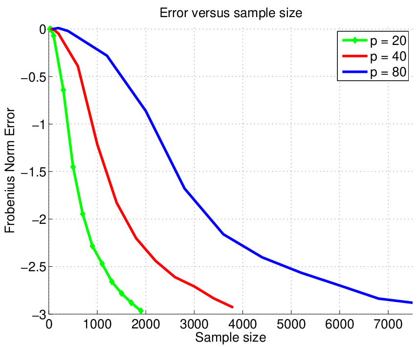
We report simulation results for three of the running examples discussed in this paper: low-rank multivariate regression, estimation in vector autoregressive processes, and matrix recovery from random projections (compressed sensing). In each case, we solved instances of the SDP for a square matrix , where for the first two examples, and for the compressed sensing example. In all cases, we considered the case of exact low rank constraints, with , and we generated by choosing the subspaces of its left and right singular vectors uniformly at random from the Grassman manifold. The observation or innovations noise had variance in each case. The VAR process was generated by first solving for the covariance matrix using the MATLAB function dylap and then generating a sample path. For each setting of , we solved the SDP for a range of sample sizes .
 |
 | |
| (a) | (b) |
Figure 1 shows results for a multivariate regression model with the covariates chosen randomly from a distribution. Panel (a) plots the Frobenius error on a logarithmic scale versus the sample size for three different matrix sizes, . Naturally, in each case, the error decays to zero as increases, but larger matrices require larger sample sizes, as reflected by the rightward shift of the curves as is increased. Panel (b) of Figure 1 shows the exact same set of simulation results, but now with the Frobenius error plotted versus the rescaled sample size . As predicted by Corollary 3, the error plots now are all aligned with one another; the degree of alignment in this particular case is so close that the three plots are now indistinguishable. (The blue curve is the only one visible since it was plotted last by our routine.) Consequently, Figure 1 shows that acts as the effective sample size in this high-dimensional setting.
Figure 2 shows similar results for the autoregressive model discussed in Example 2. As shown in panel (a), the Frobenius error again decays as the sample size is increased, although problems involving larger matrices are shifted to the right. Panel (b) shows the same Frobenius error plotted versus the rescaled sample size ; as predicted by Corollary 4, the errors for different matrix sizes are again quite well-aligned. In this case, we find (both in our theoretical analysis and experimental results) that the dependence in the autoregressive process slows down the rate at which the concentration occurs, so that the results are not as crisp as the low-rank multivariate setting in Figure 1.
 |
 | |
| (a) | (b) |
Finally, Figure 3 presents the same set of results for the compressed sensing observation model discussed in Example 3. Even though the observation matrices here are qualitatively different (in comparison to the multivariate regression and autoregressive examples), we again see the “stacking” phenomenon of the curves when plotted versus the rescaled sample size , as predicted by Corollary 5.
 |
 | |
| (a) | (b) |
6 Discussion
In this paper, we have analyzed the nuclear norm relaxation for a general class of noisy observation models, and obtained non-asymptotic error bounds on the Frobenius norm that hold under high-dimensional scaling. In contrast to most past work, our results are applicable to both exactly and approximately low-rank matrices. We stated a main theorem that provides high-dimensional rates in a fairly general setting, and then showed how by specializing this result to some specific model classes—namely, low-rank multivariate regression, estimation of autoregressive processes, and matrix recovery from random projections—it yields concrete and readily interpretable rates. Lastly, we provided some simulation results that showed excellent agreement with the predictions from our theory.
This paper has focused on achievable results for low-rank matrix estimation using a particular polynomial-time method. It would be interesting to establish matching lower bounds, showing that the rates obtained by this estimator are minimax-optimal. We suspect that this should be possible, for instance by using the techniques exploited in Raskutti et al. [39] in analyzing minimax rates for regression over -balls.
Acknowledgements
This work was partially supported by a Sloan Foundation Fellowship, AFOSR-09NL184 grant, and an NSF-CCF-0545862 CAREER grant to MJW.
Appendix A Proof of Lemma 1
Part (a) of the claim was proved in Recht et al. [41]; we simply provide a proof here for completeness. We write the SVD as , where and are orthogonal matrices, and is the matrix formed by the singular values of . By re-ordering as needed, we may assume without loss of generality that the first columns of (respectively ) correspond to the matrices (respectively ) from the statement. We then define the matrix , and write it in block form as
We now define the matrices
Note that we have
which establishes Lemma 1(a). Moreover, we note for future reference that by construction of , the nuclear norm satisfies the decomposition
| (33) |
Appendix B Proof of Lemma 3
Let denote the Euclidean sphere in -dimensions. The operator norm of interest has the variational representation
For positive scalars and , define the (random) quantity
and note that our goal is to upper bound . Note moreover that , a relation which will be useful in the analysis.
Let and denote coverings of and , respectively. We now claim that we have the upper bound
| (35) |
To establish this claim, we note that since the sets and are -covers, for any pair , there exists a pair such that and , with . Consequently, we can write
| (36) |
By construction, we have the bound , and similarly as well as . Substituting these bounds into the decomposition (36) and taking suprema over the left and right-hand sides, we conclude that
from which the bound (35) follows.
We now apply the union bound to control the discrete maximum. It is known (e.g., [29, 33]) that there exists a covering of and with at most and elements respectively. Consequently, we have
| (37) |
It remains to obtain a good bound on the quantity , where are arbitrary but fixed. Since has i.i.d. elements and is fixed, we have for each . These variables are independent of one another, and of the random matrix . Therefore, conditioned on , the sum is zero-mean Gaussian with variance
Define the event . Using Lemma 2, we have with probability at least , which implies that . Therefore, conditioning on the event and its complement , we obtain
Combining this tail bound with the upper bound (37), we have
Setting , this probability vanishes as long as .
Appendix C Technical details for Corollary 4
C.1 Proof of Lemma 4
Recalling that denotes the unit-norm Euclidean sphere in -dimensions, we first observe that . Our next step is to reduce the supremum to a maximization over a finite set, using a standard covering argument. Let denote a -cover of it. By definition, for any , there is some such that , where . Consequently, for any , the triangle inequality implies that
and hence that . Re-arranging yields the useful inequality
| (38) |
Using inequality (38), we have
| (39) |
where the last inequality follows from the union bound, and the fact [29, 33] that there exists a -covering of with at most elements.
In order to complete the proof, we need to obtain a sharp upper bound on the quantity , valid for any fixed . Define the random vector with elements . Note that is zero mean, and its covariance matrix has elements . In order to bound the spectral norm of , we note that since it is symmetric, we have , and moreover
Combining the pieces, we obtain
| (40) |
Moreover, we have . Applying Lemma 8 with , we conclude that
Combined with the bound (39), we obtain
| (41) |
with probability at least , which establishes the upper bound (28)(a).
Turning to the lower bound (28)(b), we let be an -cover of for some to be chosen. Thus, for any , there exists some such that , and . Define the function via , and note that . With this notation, we have
since . Since , we obtain the lower bound
By the previously established upper bound(28)(a), have with high probability. Hence, choosing ensures that .
Consequently, it suffices to lower bound the minimum over the covering set. We first establish a concentration result for the function that holds for any fixed . Note that we can write
As before, if we define the random vector with elements , then with . Moreover, we have . Consequently, applying Lemma 8 yields
Note that this bound holds for any fixed . Setting and applying the union bound yields that
which vanishes as long as .
C.2 Proof of Lemma 5
Let denote the Euclidean sphere in -dimensions, and for positive scalars and , define the random variable . Note that our goal is to upper bound . Let and denote coverings of and , respectively. Following the same argument as in the proof of Lemma 3, we obtain the upper bound
| (42) |
We now apply the union bound to control the discrete maximum. It is known (e.g., [29, 33]) that there exists a covering of with at most elements. Consequently, we have
| (43) |
It remains to obtain a tail bound on the quantity , for any fixed pair .
For each , let and denote the row of and . Following some simple algebra, we have the decomposition , where
We may now bound each in turn; in doing so, we make repeated use of Lemma 8, which provides concentration bounds for a random variable of the form , where for some matrix .
Bound on :
We begin with , which the easiest to control since (up to scaling by ), it corresponds to the deviation away from the mean of -variable with degrees of freedom. Consequently, applying Lemma 8 with , we obtain
| (44) |
Bound on :
We can write the term as a deviation of from its mean, where in this case the covariance matrix is no longer the identity. In concrete terms, let us define a random vector with elements . As seen in the proof of Lemma 4 from Appendix C.1, the vector is zero-mean Gaussian with covariance matrix such that (see equation (40)). Since we have , applying Lemma 8 yields that
| (45) |
Bound on :
To control this quantity, let us define a zero-mean Gaussian random vector with elements . This random vector has covariance matrix with elements
where is the Kronecker delta for the event . As before, by symmetry of , we have , and hence
Morever, we have , so that by applying Lemma 8, we conclude that
| (46) |
which completes the analysis of this term.
Appendix D Proof of Proposition 1
Note that , and that since the claim (21) is invariant to rescaling, it suffices to prove it for all with . Letting be a given radius, we seek lower bounds on the quantity
In particular, our goal is to prove that for any , the lower bound
| (48) |
holds with probability at least . By a standard peeling argument (see Raskutti et al. [39] for details), this lower bound implies the claim (21).
We establish the lower bound (48) using Gaussian comparison inequalities [29] and concentration of measure (see Lemma 7). For each pair , consider the random variable , and note that it is Gaussian with zero mean. For any two pairs and , some calculation yields
| (49) |
We now define a second Gaussian process via
where and are independent with i.i.d. entries. By construction, is zero-mean, and moreover, for any two pairs and , we have
| (50) |
It can be shown that for all pairs , we have
| (51) |
Moreover, equality holds whenever . The conditions of the Gordon-Slepian inequality [29] are satisfied, so that we are guaranteed that
| (52) |
We compute
Since has i.i.d. entries, standard random matrix theory [16] implies that . Putting together the pieces, we conclude that
Finally, we need to establish sharp concentration around the mean. Note that the function is Lipschitz with constant , so that Lemma 7 implies that
Setting yields the claim.
Appendix E Some useful concentration results
The following lemma is classical [29, 32], and yields sharp concentration of a Lipschitz function of Gaussian random variables around its mean.
Lemma 7.
Let have i.i.d. entries, and let and be Lipschitz with constant (i.e., ). Then for all , we have
By exploiting this lemma, we can prove the following result,
which yields concentration of the squared -norm of an
arbitrary Gaussian vector:
Lemma 8.
Given a Gaussian random vector , for all , we have
| (53) |
Proof.
Let be the symmetrix matrix square root, and consider the function . Since it is Lipschitz with constant , Lemma 7 implies that
| (54) |
By integrating this tail bound, we find that the variable satisfies the bound , and hence conclude that
| (55) |
Combining this bound with the tail bound (54), we conclude that
| (56) |
References
- [1] J. Abernethy, F. Bach, T. Evgeniou, and J. Stein. Low-rank matrix factorization with attributes. Technical Report Technical Report N-24/06/MM, Ecole des mines de Paris, France, September 2006.
- [2] A. A. Amini and M. J. Wainwright. High-dimensional analysis of semdefinite relaxations for sparse principal component analysis. Annals of Statistics, 5B:2877–2921, 2009.
- [3] C. W. Anderson, E. A. Stolz, and S. Shamsunder. Multivariate autoregressive models for classification of spontaneous electroencephalogram during mental tasks. IEEE Trans. on bio-medical engineering, 45(3):277, 1998.
- [4] T. W. Anderson. The statistical analysis of time series. Wiley Classics Library. John Wiley and Sons, New York, 1971.
- [5] A. Argyriou, T. Evgeniou, and M. Pontil. Multi-task feature learning. In Neural Information Processing Systems (NIPS), Vancouver, Canada, December 2006.
- [6] F. Bach. Consistency of trace norm minimization. Journal of Machine Learning Research, 9:1019–1048, June 2008.
- [7] P. Bickel and E. Levina. Covariance estimation by thresholding. Annals of Statistics, 2008. To appear.
- [8] P. Bickel and E. Levina. Regularized estimation of large covariance matrices. Annals of Statistics, 36(1):199–227, 2008.
- [9] P. Bickel, Y. Ritov, and A. Tsybakov. Simultaneous analysis of lasso and dantzig selector. Annals of Statistics, 2009. To appear.
- [10] S. Boyd and L. Vandenberghe. Convex optimization. Cambridge University Press, Cambridge, UK, 2004.
- [11] E. N. Brown, R. E. Kass, and P. P. Mitra. Multiple neural spike train data analysis: state-of-the-art and future challenges. Nature Neuroscience, 7(5), May 2004.
- [12] E. Candes and T. Tao. Decoding by linear programming. IEEE Trans. Info Theory, 51(12):4203–4215, December 2005.
- [13] E. J. Candès and B. Recht. Exact matrix completion via convex optimization. CoRR, abs/0805.4471, 2008.
- [14] S. Chen, D. L. Donoho, and M. A. Saunders. Atomic decomposition by basis pursuit. SIAM J. Sci. Computing, 20(1):33–61, 1998.
- [15] A. Cohen, W. Dahmen, and R. DeVore. Compressed sensing and best k-term approximation. J. of. American Mathematical Society, 22(1):211–231, July 2008.
- [16] K. R. Davidson and S. J. Szarek. Local operator theory, random matrices, and Banach spaces. In Handbook of Banach Spaces, volume 1, pages 317–336. Elsevier, Amsterdan, NL, 2001.
- [17] D. Donoho. Compressed sensing. IEEE Trans. Info. Theory, 52(4):1289–1306, April 2006.
- [18] N. El-Karoui. Operator norm consistent estimation of large dimensional sparse covariance matrices. Technical Report 734, UC Berkeley, Department of Statistics, 2007.
- [19] M. Fazel. Matrix Rank Minimization with Applications. PhD thesis, Stanford, 2002. Available online: http://faculty.washington.edu/mfazel/thesis-final.pdf.
- [20] J. Fisher and M. J. Black. Motor cortical decoding using an autoregressive moving average model,. IEEE Engineering in Medicine and Biology Society, pages 1469–1472, September 2005.
- [21] J. Friedman, T. Hastie, and R. Tibshirani. Sparse inverse covariance estimation with the graphical Lasso. Biostatistics, 2007.
- [22] L. Harrison, W. D. Penny, and K. Friston. Multivariate autoregressive modeling of fmri time series. NeuroImage, 19:1477–1491, 2003.
- [23] R. A. Horn and C. R. Johnson. Matrix Analysis. Cambridge University Press, Cambridge, 1985.
- [24] R. A. Horn and C. R. Johnson. Topics in Matrix Analysis. Cambridge University Press, Cambridge, 1991.
- [25] J. Huang and T. Zhang. The benefit of group sparsity. Technical Report arXiv:0901.2962, Rutgers University, January 2009.
- [26] S. Ji and J. Ye. An accelerated gradient method for trace norm minimization. In International Conference on Machine Learning (ICML), New York, NY, USA, 2009. ACM.
- [27] I. M. Johnstone. On the distribution of the largest eigenvalue in principal components analysis. Annals of Statistics, 29(2):295–327, April 2001.
- [28] R. H. Keshavan, A. Montanari, and S. Oh. Matrix completion from noisy entires. Preprint available at http://arxiv.org/abs/0906.2027v1, 2009.
- [29] M. Ledoux and M. Talagrand. Probability in Banach Spaces: Isoperimetry and Processes. Springer-Verlag, New York, NY, 1991.
- [30] K. Lounici, M. Pontil, A. B. Tsybakov, and S. van de Geer. Taking advantage of sparsity in multi-task learning. Technical Report arXiv:0903.1468, ETH Zurich, March 2009.
- [31] H. Lütkepolhl. New introduction to multiple time series analysis. Springer, New York, 2006.
- [32] P. Massart. Concentration Inequalties and Model Selection. Ecole d’Eté de Probabilités, Saint-Flour. Springer, New York, 2003.
- [33] J. Matousek. Lectures on discrete geometry. Springer-Verlag, New York, 2002.
- [34] N. Meinshausen and P. Bühlmann. High-dimensional graphs and variable selection with the Lasso. Annals of Statistics, 34:1436–1462, 2006.
- [35] S. Negahban, P. Ravikumar, M. J. Wainwright, and B. Yu. A unified framework for high-dimensional analysis of M-estimators with decomposable regularizers. In Proceedings of the NIPS Conference, Vancouver, Canada, December 2009.
- [36] Y. Nesterov. Gradient methods for minimizing composite objective function. Technical Report 2007/76, CORE, Universit’e catholique de Louvain, 2007.
- [37] G. Obozinski, M. J. Wainwright, and M. I. Jordan. Union support recovery in high-dimensional multivariate regression. Annals of Statistics, To appear. Presented in part at NIPS 2008 conference.
- [38] D. Paul and I. Johnstone. Augmented sparse principal component analysis for high-dimensional data. Technical report, UC Davis, January 2008.
- [39] G. Raskutti, M. J. Wainwright, and B. Yu. Minimax rates of estimation for high-dimensional linear regression over -balls. Technical Report arXiv:0910.2042, UC Berkeley, Department of Statistics, 2009. Presented in part at Allerton Conference, Sep. 2009.
- [40] P. Ravikumar, M. J. Wainwright, G. Raskutti, and B. Yu. High-dimensional covariance estimation: Convergence rates of -regularized log-determinant divergence. Technical report, Department of Statistics, UC Berkeley, September 2008. Presented in part at NIPS 2008.
- [41] B. Recht, M. Fazel, and P. A. Parrilo. Guaranteed minimum-rank solutions of linear matrix equations via nuclear norm minimization. SIAM Review, 2007. to appear.
- [42] A. J. Rothman, P. J. Bickel, E. Levina, and J. Zhu. Sparse permutation invariant covariance estimation. Electronic Journal of Statistics, 2009.
- [43] N. Srebro, J. Rennie, and T. Jaakkola. Maximum-margin matrix factorization. In Proceedings of the NIPS Conference, Vancouver, Canada, 2005.
- [44] N. Srebro, J. Rennie, and T. S. Jaakkola. Maximum-margin matrix factorization. In Neural Information Processing Systems (NIPS), Vancouver, Canada, December 2004.
- [45] R. Tibshirani. Regression shrinkage and selection via the lasso. Journal of the Royal Statistical Society, Series B, 58(1):267–288, 1996.
- [46] L. Vandenberghe and S. Boyd. Semidefinite programming. SIAM Review, 38:49–95, 1996.
- [47] M. J. Wainwright. Sharp thresholds for high-dimensional and noisy sparsity recovery using -constrained quadratic programming (Lasso). IEEE Trans. Information Theory, 55:2183–2202, May 2009.
- [48] M. Yuan and Y. Lin. Model selection and estimation in regression with grouped variables. Journal of the Royal Statistical Society B, 1(68):49, 2006.
- [49] M. Yuan and Y. Lin. Model selection and estimation in the Gaussian graphical model. Biometrika, 94(1):19–35, 2007.