Physical problems for future Photon Colliders
Abstract
In this report I discuss physical problems for future Photon Colliders (PLC), which can be stated AFTER 10 years of work of LHC and few years of work of ILC. I discuss mainly the unfavorable case when these colliders will give us only Higgs boson(s) and perhaps some charged particles of unclear nature. I focus my attention for the case of PLC based on the second stage of ILC (about 1 TeV) or CLIC (1-3 TeV). It offers opportunity to study new series of fundamental physical problems. Among them – multiple production of gauge bosons, hunt for strong interaction in Higgs sector, search of exotic interactions in the process with final photons having transverse momenta .
1 Introduction. Different opportunities for PLC
We discuss here Photon Colliders (PLC) for different energy ranges. To do that, we start with

repetition of basic scheme [1]. The focused laser flash meet the electron bunch of LC in the conversion point C at small distance before interaction point IP. In C a laser photon scatters on high–energy electron taking from it a large portion of energy. Scattered photons travel along the direction of the initial electron with angular spread , they are focused in the IP. Here they collide with opposite electron ( collider) or photon ( collider).
For the ILC-1 based PLC, the laser flash with energy of a few Joules and length of a few mm is sufficient. The preferable form of basic electron beam for PLC is different from that for LC. Based on that generally one can make the luminosity of PLC even larger than that of basic LC. For discussed realizations this opportunity is used only weakly. The total additional cost is estimated in this case as % from that of LC [4].
The energy spectrum of obtained photon beam is concentrated near its upper bound. If – electron energy and , then . Spectrum become more sharp with suitable choice of polarizations of initial electrons and laser photons and with growth of . The obtained photon beam is strongly polarized. The photon energy and mean photon helicity spectra are presented in Fig. 2 in dependence on for the case when initial electron helicity and initial lase photons are right polarized (helicity ) for two values .


The real picture is more complex.
(i) When photons
with energy propagate from collision
point C to interaction point IP, they distribute over the
wider area reducing luminosity in its soft part.
(ii) The low energy part of spectra is increased due
to multiple rescatterings of electron on the other laser
photons.
(iii) The nonlinear QED effects also modify
spectra, mainly for the case .
(iv) At some fraction of produced photons disappear in the collision with laser photon, . This effect result in strong limitation for the practical conversion coefficient.
In future practice, the luminosity/polarization spectra must be measured during operations.
The production of photon beam for the LC with the electron energy GeV offer difficult problems making construction of PLC for this energy range doubtful [2]. We consider here briefly two main ways of production of photon beams for TeV [3].
The first way is to use classical conversion scheme [1] with infrared laser or FEL to reach the highest luminosity. The laser photon energy will be 0.5-0.2 eV with which prevents pair production in collision of high energy and laser photons. To get high conversion coefficient, the conversion process has to take place with large non-linear QED effects, making final photon distributions less monochromatic and less polarized. Here one must work with infrared optics which causes additional difficulties (see discussion e.g. in [2]).
The second way is to use the same laser (and the same optics) as for the electron beam energy 250 GeV (ILC-1) – with photon energy eV – but limit ourselves by a small conversion coefficient (at x=18) [3]. This value assures that the losses of high energy photons due to pair production in collision of high energy photon with laser photon are small. At this value of conversion coefficient the non-linear QED effects are insignificant and contribution from rescatterings is small. Here the maximum photon energy is higher than in the first way, , energy distribution of high energy photons is more sharp, etc., right fig. 2. These advantages allow to consider this option despite the reduction of luminosity by about one order in comparison with the first way. The second way seems more attractive to me.
The typical expected parameters of PLC for these two ways are presented in the Table. Here lines D-G describe only the high energy peak (), which is separated well from low energy part of spectrum and luminosity, it depends only weakly on details of conversion scheme. In both schemes one can hope to have annual luminosity fb-1/year.
| Way | I, | II, | |
|---|---|---|---|
| A | Necessary laser flash energy (J) | ||
| B | The conversion coefficient | 0.7 | 0.15 |
| C | Maximal photon energy | ||
| D | Luminosity | 0.35 | |
| E | Luminosity | 0.25 | 0.2 |
| F | Mean energy spread | 0.07 | 0.03 |
| G | Mean photon helicity | 0.95 | 0.95 |
The set of problems for PLC at ILC1 is widely discussed (see e.g. [4]). The study of some of them (with increase of thresholds for search of new particles) will be a natural task for PLC with higher beam energy. We select here problems to answer for questions: what new can be studied at PLC AFTER about 10 years of work of LHC with higher beam energy, and perhaps, few years of work of ILC with slightly larger beam energy and luminosity.
2 QCD and hadron physics
Photon structure function is unique object of QCD, calculable at large enough without additional phenomenological parameters [6]. It can be measured at PLC in mode with high accuracy, since photon target with its energy and polarization here are practically known. The manipulation with beam polarizations will be important instrument here.
The region of electron transverse momenta above 50 GeV () can be studied well, providing opportunity to study effect of -boson exchange and interference.
The other studies like those at HERA are possible here.
3 Higgs physics
Higgs mechanism of EWSB can be realized either by minimal Higgs sector with one observable neutral scalar Higgs boson (SM) or by non-minimal Higgs sector with larger number of observable scalars. In this section for definiteness we consider SM and specific non-minimal Higgs sector – Two Higgs Doublet Model (2HDM). The latter is the simplest extension of Higgs sector of SM. It contains 2 complex Higgs doublet fields and with v.e.v.’s and . The physical sector contains charged scalars and three neutral scalars , generally having no definite parity. In the CP conserving case these three become two scalars , () and a pseudoscalar . For definiteness, we assume the Model II for the Yukawa coupling in 2HDM (the same is realized in MSSM).
SM-like scenario. Distinguishing models.
Let earlier observations discover Higgs boson, similar to that in SM (SM-like scenario). How to state whether we deal with SM Higgs boson or some other realization of Higgs sector (e.g. 2HDM)? What can we say about properties of this realization?
LHC can measure Higgs couplings to particles only with low precision, typically 10-20%. The LC will improve these results up to 5-10%, sometimes better. The PLC can improve these accuracies further to about 2%.
Here, measuring the () couplings is very promising. The expected accuracy in the measurement of the two-photon width is 2% at GeV and fb-1 (by 5 times lower than the anticipated annual luminosity) [7].
Example – distinguishing SM/2HDM. The SM – like scenario means that the

coupling constants squared, measured at LHC and LC, are close to the SM value within anticipated precision, (not coupling constants themselves!. In the 2HDM this scenario can be realized in many ways.
The models can be distinguished via measurement of the width of the observed SM-like Higgs boson, fig. 3 [8]. In this figure we show the ratio of to its SM value for one typical class of realization of SM-like scenario. The bands reflect the anticipated uncertainty of future measurements. The deviation from , given by contributions of heavy charged Higgs bosons for a natural set of parameters, is about % (compare with anticipated 2% accuracy). For the other sets of parameters, consistent with SM-like scenario, the deviation from is even larger.
CP violation in Higgs sector.
In many extensions of Higgs model (e.g. in 2HDM) observable neutral Higgs bosons have generally no definite CP-parity and effectively
| (1) |
Here and are the standard field strength for the electromagnetic field. The relative effective couplings and are described with standard triangle diagram , they are expressed with known equations via masses of charged fermions and W, and mixing parameters (parameters of 2HDM potential). They are generally complex ( –loop).
Total production cross section varies strong with variation of circular and linear polarizations of photon beams and the angle between linear polarization vectors [9]:
| (2) |

In particular, violation of CP symmetry in the Higgs sector leads to difference in the production cross sections in the collision of photons with identical total helicity (0) but with opposite helicities of separate photons:
| (3) |
Standard calculation of vertexes in the 2HDM at different parameters of model gives typical dependence, shown in fig. 4 at . It is seen that effect is strong and can be measured well.
Observation of strong interaction in Higgs sector in process at not too high energy.
At high values of Higgs boson self-coupling constant, the Higgs mechanism of Electroweak Symmetry Breaking in Standard Model (SM) can be realized without actual Higgs boson but with strong interaction in Higgs sector (SIHS) which will manifest itself as a strong interaction of longitudinal components of and bosons. It is expected that this interaction will be seen in the form of , and resonances at TeV. Main efforts to discover this opportunity are directed towards the observation of such resonant states. It is a difficult task for the LHC due to high background and it cannot be realized at the energies reachable at the ILC in its initial stages.
This strong interaction can be observed in the study of the charge asymmetry of produced in the process similar to that which was discussed in low energy pion physics [12], [13]. To explain the set up of the problem we discuss this process in SM [14].
We subdivide the diagrams of the process into three groups, where subprocesses of main interest are shown in boxes, sign represents next stage of process.
a) Diagrams contain subprocesses and , modified by the strong interaction in the Higgs sector (two–gauge ).
b) Diagrams contain subprocesses and , modified by the strong interaction in the Higgs sector (one–gauge).
c) Diagrams are prepared by connecting the photon line to each charged particle line to the diagram shown inside the box. Strong interaction does not modify this contribution. These contributions are switched off at suitable electron polarization.
The subprocess (from contribution a)) produces C-even system , the subprocess (from contribution b)) produces C-odd system . The interference of similar contributions for the production of pions is responsible for large enough charge asymmetry, very sensitive to the phase difference of S (D) and P waves in scattering, [12]. This very phenomenon also takes place in the discussed case of ’s. However, for the production of subprocesses with the replacement of are also essential. Therefore, the final states of each type have no definite -parity. Hence, charge asymmetry appears both due to interference between contributions of types a) and b) and due to interference of and contributions each within their own types.
Asymmetries in SM. To observe the main features of the effect of charge asymmetry and its potential for the study of strong interaction in the Higgs sector, we calculated some quantities describing charge asymmetry for collision at GeV with polarized photons. We used CalcHEP package [17] for simulation.
We denote by momenta of , by – momentum of the scattered electron and , . We present below dependence of charge asymmetric quantity on . The -dependencies for the other charge asymmetric quantities have similar qualitative features [14].
We applied the cut in transverse momentum of the scattered electron,
| (4) |
Observation of the scattered electron allows to check kinematics completely.
 |
 |
 |
| GeV | GeV | GeV, without |
| one-gauge contributions |
Influence of polarization. Fig. 5 (left and central plots) represents distribution in variable on photon polarization and cut in . We did not study the dependence on electron polarization. This dependence is expected to be weak in SM where main contribution to cross section is given by diagrams of type a) with virtual photons having the lowest possible energy. These photons ”forget” the polarization of the incident electron. The strong interaction contribution becomes essential at highest effective masses of system with high energy of virtual photon or , the helicity of which reproduces almost completely the helicity of incident electron [18]. The study of this dependence will be a necessary part of studies beyond SM.
Significance of different contributions. To understand the extent of the effect of interest, we compared the entire distribution in variable with that without one-gauge contribution at GeV (right plot in Fig. 5). Strong interaction in the Higgs sector modifies both one–gauge and two–gauge contributions. The study of charge asymmetry caused by their interference will be a source of information on this strong interaction. One can see that one–gauge contribution is so essential that neglecting on it even changes the sign of charge asymmetry (compared to that for the entire process). Therefore, the charge asymmetry is very sensitive to the interference of two–gauge and one–gauge contributions which is modified under the strong interaction in the Higgs sector. The measurement of this asymmetry will be a source of data on the phase difference of different partial waves of scattering.
If more than one scalar, like Higgs boson, will be observed,
it will be strong argument in favor of more complex Higgs sector, like 2HDM or something else. It is necessary to measure properties of these scalars, including coupling to fermions, gauge bosons and self-couplings with the best accuracy, to find what model is realized.
To understand properties of model, one must first to measure masses all scalars and their coupling to gauge bosons and some fermions. However, even these data are non-sufficient for fixing of parameters of model. Usually for this goal somebody suggest to measure triple Higgs coupling in the processes like , . However their cross sections are typically low and contributions of triple Higgs vertexes there is added by contributions of product of other Higgs vertexes. Moreover, knowledge of this vertex is non-sufficient for fixing of parameters of the model. It was found in [15] the complete set of observable parameters of 2HDM can be extracted from masses of and 3 neutrals , , (generally with no definite CP parity) and charged Higgs , their couplings to gauge bosons, added by 3 triple Higgs couplings (like or ) and one quartic coupling (like ). At high enough energy of PLC the cross sections of processes are without interference withe other vertexes and they are not small. One can hope also to measure coupling via measuring of production cross section.
The information of the complete set of parameters of model will give also information about way of evolution of phase states of earlier Universe [16].
4 New particles
New charged particles will be discovered at LHC and in mode of LC. We expect their decay for final states with invisible particles (like LSP in MSSM).
How to measure mass, decay modes and spin of these new particles?
In these problems the production provides essential advantages compared to collisions
How to observe signals from new neutral particles – possible candidates for dark matter?
The cross section of the pair production ( – scalar, – fermion, – gauge boson) not far from the threshold is given by QED with reasonable accuracy.

These cross sections decreases slowly with energy growth. Therefore, they can be studied relatively far from the threshold where the decay products are almost non-overlapping.
Near the threshold with + sign for and – sign for . This polarization dependence provides the opportunity to determine spin of produced particle in the experiments with longitudinally polarized photons.
The polarization of produced fermion or vector depends on the initial photon helicity. At the decay this polarization is transformed into the momentum distribution of decay products. E.g., for the SM processes like (obtained from muon decay modes of , , etc.) muons should exhibit charge asymmetry linked to the polarization of initial photons – see sect. 4. These studies can help to understand the nature of candidates for Dark Matter particles.
The possible CP violation in the interaction can be seen as a variation of cross section with changing the sign of both photon helicities (like in fig. 4).
Charge asymmetry in processes ,
In the SM the effect appears due to P nonconservation in the W-decay.
We select events with two cuts, for escape angle for each observed particle and for transverse momentum of each observed particle and for missed transverse momentum
| (5) |
These simultaneous cuts allow to eliminate many backgrounds. We used mrad and study dependence of effect starting from GeV.

The fig. 7 demonstrates the charge asymmetry in the collision of two left polarized photons at GeV, left and right plots show distributions for negative and positive muons respectively. We find that effect is strong and well observable even at large enough GeV (the results were obtained with the aid of CalcHEP package [11]). So, one can conclude that this charge asymmetry is huge and well observable effect in SM. The study of dependence of effect shows that one can hope to see effects of New Physics in these asymmetries at high transverse momenta (larger than 100 GeV).
5 Multiple production of SM gauge bosons
The observation of pure interactions of SM gauge bosons (W and Z) or their interaction with leptons will allow to check SM with higher accuracy and observe signals of New Physics. The most ambitious goal is to find deviations from predictions of SM caused by New Physics
interactions (and described by anomalies in effective Lagrangian). There are many anomalies relevant to the gauge boson interactions. Each process is sensitive to some group of
anomalies. Large variety of processes obtainable at
PLC’s allows to separate anomalies from each
other.
The high energy PLC is the only collider among different future accelerators where one can measure large number of different processes of such type with high enough accuracy.
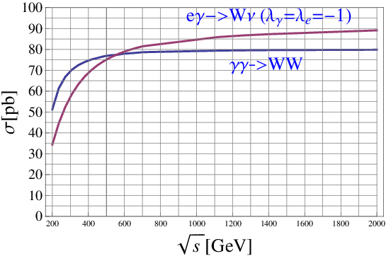
2-nd order processes. The cross sections of basic processes and are so high
(Fig. 8) that one can expect to obtain about events per year providing accuracy better than 0.1%.
The cross sections are almost independent of energy and
photon polarization
[5]. However, final distributions depend on polarization strongly [11].
The accuracy of measurement of these cross sections is sufficient to study in detail 2-loop radiative corrections. Together with standard problems of precise calculations one can note here two non-trivial problems, demanding detailed theoretical study:
(i) construction of
–matrix for system with unstable particles;
(ii) gluon corrections like Pomeron exchange between
quark components of ’s.
The mentioned high values of cross sections of the 2-nd order processes make it possible to measure their multiple ”radiative derivatives” — processes of the 3-rd and 4-th order, depending in different ways on various anomalous contributions to the effective Lagrangian.
3-rd order processes. We consider here 3 processes (fig. 9a). Total cross section
 |
 |
| (a) 3-rd order processes | (b) 4-th order processes |
. It is very high and easily estimated by equivalent photon method. This large contribution is not very interesting, being only a cross section of averaged with some weight. However, at large enough transverse momentum of scattered electron this factorization is violated. Because of it we present only for GeV. Even this small fraction of total cross section appears so large that it allows to separate contribution of subprocess.
4-th order processes. The cross sections of these processes (Fig. 9b) are high enough to measure them with 1% precision. For the same reason as for process we present cross section for process only for GeV. Even this small fraction of total cross section appears so large that it allows to separate contribution of subprocess.
The study of the 2-nd order processes will allow to extract some anomalous parameters or their combinations. The study of the 3-rd order processes will allow to enlarge the number of extracted anomalous parameters and separate some of combinations extracted from the 2-nd order processes. The study of the 4-th order processes will again enlarge the number of separated anomalous parameters.
6 Large angle high energy photons for exotics
The PLC allows to observe signals from the whole group of exotic models of New Physics in one common experiment. These are models with large extra dimensions [19], point-like monopole [20], unparticles [21]. All these models have common signature – the cross section for production grows with energy as () and the photons are produced

almost isotropically. Future observations either will give limits for scales of these exotics or will allow to see these effects by recording large photons11 1 In my personal opinion it is hardly probable that these models describe reality.. The study of dependence on initial photon polarization will be useful to separate the mechanisms.
All these exotics at modern day energies can be described by effective point-like interaction of Fig. 10:
| (6) |
In different models different orders of field indices are realized, is characteristic mass scale, expressed via parameters of model. (In all cases , and – channels are essential.)
Let us describe main features of matrix element (in the photon c.m.s.):
gauge invariance provides factor for each photon
leg;
to make this factor dimensionless it should be written as
. Therefore, the amplitude .
The characteristic scale is large enough not to contradict modern day data. It accumulates other coefficients.
The cross section
| (7) |
reference Tevatron D0 175 GeV [22] LHC 2 TeV [20] (100 fb-1) [20] LC (1000 fb-1) [20]
with smooth function , describing some composition of S and P-waves, dependent on details of model, and For large extra dimensions and monopoles entire dependence is given by the factor from (7), for unparticles additional factor is added.
For the large extra dimensions case the point in Fig. 10 describes an elementary interaction, given by product of stress-energy tensors for the incident and the final photons, that are exchanging the tower of Kaluza-Klein excitations (with permutations), i.e. . After averaging over polarizations for tensorial KK excitations
| (8) |
Unlike to ILC1, at high energy PLC the other channels (like ) are less sensitive to the extra dimension effect.
The point–like Dirac monopole existence would explain mysterious quantization of an electric charge since in this case with . There is no place for this monoplle in modern theories of our world but there are no precise reasons against its existence. In this case the point in Fig. 10 corresponds to exchange of loop of heavy monopoles (like electron loop in QED – Heisenberg–Euler type lagrangian).
Let be monopole mass. At the electrodynamics of monopoles is expected to be similar to the standard QED with effective perturbation parameter [20]. The scattering is described by monopole loop, and it is calculated within QED,
The coefficients and details of angular and polarization dependence depend strongly on the spin of the monopole.
After averaging over polarizations, the dependence and total cross section is described by the same equations as for the extra dimensions case. The parameter is expressed via monopole mass and coefficient , dependent on monopole spin ():
| (9) |
Unparticle is an object, describing particle scattering via propagator which has no poles at real axis. It was introduced in 2007 [21]. This propagator behaves (in the scalar case) as where scalar dimension is not integer or half-integer. The interaction carried by unparticle is described as with some phase factor. For matrix element it gives
| (10) |
The anticipated discovery limits for all these models are shown in the Table 2. The results of D0 experiment [22], recalculated to used notations, are also included here. For the unparticle model presented numbers are modified by corrections .
This paper is supported by grants RFBR 08-02-00334-a, NSh-1027.2008.2, Program of Dept. of Phys. Sc RAS ”Experimental and theoretical studies of fundamental interactions related to LHC” and INFN grant.
References
- [1] I.F. Ginzburg, G.L. Kotkin, V.G. Serbo, V.I. Telnov. Nucl. Instr. Meth. 205 (1983) 47–68; I.F. Ginzburg, G.L. Kotkin, S.L. Panfil, V.G. Serbo, V.I. Telnov. Nucl. Instr. Meth. 219 (1983) 5.
- [2] V. Telnov. hep-ex/0012047
- [3] I.F. Ginzburg, G.L. Kotkin, V.G. Serbo, in preparation
- [4] B. Badelek et al. TESLA TDR hep-ex/0108012
- [5] I.F. Ginzburg, G.L. Kotkin, S.L. Panfil, V.G. Serbo. Nucl. Phys. B228 (1983) 285
- [6] E. Witten, Nucl. Phys. B120 (1977) 189.
- [7] G. Jikia, S. Söldner-Rembold, Nucl. Phys. B (Proc. Suppl.) 82 (2000) 373; M. Melles, W.J. Stirling, V.A. Khoze,Phys. Rev. D61(2000) 054015
- [8] I.F. Ginzburg, M. Krawczyk, P.Osland. Nucl. Instr Meth. A 472 (2001) 149–154; hep-ph/0101229
- [9] I.F.Ginzburg, I.P. Ivanov, Eur. Phys. J. C 22 (2001) 411-421)
- [10] I.F. Ginzburg, V.A.Ilyin, A.E.Pukhov, V.G.Serbo, S.A.Shichanin. Phys. At. Nucl.– Russian Yad Fiz. 56 (1993) 57–63.
- [11] D. A. Anipko, I. F. Ginzburg, K.A. Kanishev, A. V. Pak, M. Cannoni, O. Panella. Phys. Rev. D 78 (2008) 093009; ArXive: hep-ph/0806.1760
- [12]
V.L. Chernyak, V.G. Serbo, Nucl. Phys. B 67
(1973) 464;
I.F.Ginzburg, A.Schiller, V.G. Serbo, Eur. Phys. J. C18 (2001) 731 - [13] I.F.Ginzburg, Proc. 9th Int. Workshop on Photon-Photon Collisions, San Diego (1992) 474
- [14] I.F. Ginzburg, K.A. Kanishev, hep-ph/0507336
- [15] K.A. Kanishev, in preparation
- [16] I.F. Ginzburg, I.P. Ivanov, K.A. Kanishev, hep-ph/0911.2383
- [17] A. Pukhov. hep-ph/0412191
- [18] I.F. Ginzburg, V.G. Serbo. Phys. Lett. B 96 (1980) 68-70.
- [19] K.R. Dienes, E. Dudas, T. Gherghetta. hep-ph/9803466, Phys. Lett. B 436 (1998); M. Shifman. hep-ph/09073074
- [20] I.F. Ginzburg, S.L. Panfil. Sov. Yad. Fiz. 36 (1982) 850; I.F. Ginzburg, A. Schiller. Phys. Rev. D 60 (1999) 075016
- [21] H. Georgy, Phys. Rev. Let. 98 (2007) 221601;hep-ph/0703.260; I.Sahin, S.C. Inan, hep-ph/09073290
- [22] B. Abbot et al. Phys. Rev. Lett. 81 (1998) 524, hep-ex/9803023