Modeling and simulation with operator scalingThanks: M. M. Meerschaert was partially supported by NSF grants DMS-0803360 and EAR-0823965. J. Rosiński was partially supported by NSA grant MSPF-50G-049. S. Cohen wishes to thank the Department of Mathematics, University of Tennessee, for their hospitality during a visit that initiated this project.
Abstract.
Self-similar processes are useful in modeling diverse phenomena that exhibit scaling properties. Operator scaling allows a different scale factor in each coordinate. This paper develops practical methods for modeling and simulating stochastic processes with operator scaling. A simulation method for operator stable Lévy processes is developed, based on a series representation, along with a Gaussian approximation of the small jumps. Several examples are given to illustrate practical applications. A classification of operator stable Lévy processes in two dimensions is provided according to their exponents and symmetry groups. We conclude with some remarks and extensions to general operator self-similar processes.
Key words and phrases:
Lévy processes, Gaussian approximation, shot noise series expansions, simulation, tempered stable processes, operator stable processes.1. Introduction
Self-similar processes form an important and useful class, favored in practical applications for their nice scaling properties, see for example the recent books of Embrechts and Maejima [11] and Sheluhin et al. [44]. In finance, self-similar processes such as fractional Brownian motion and stable Lévy motion are used to model prices (or log returns). Recall that a stochastic process taking values in is self-similar if
| (1.1) |
at every scale . Here indicates equality of finite dimensional distributions, and we assume is stochastically continuous with . The parameter is often called the Hurst index [14]. Operator self-similar processes allow the scaling factor (Hurst index) to vary with the coordinate. Therefore, a process as above is said to be operator self-similar (o.s.s.) if there exists a linear operator such that
| (1.2) |
for all , where the matrix power . The linear operator in (1.2) is called an exponent of the operator self-similar process . If for some , then is self-similar. If is diagonal, then the marginals of are self-similar, and the Hurst index can vary with the coordinate. This is important in modeling many real world phenomena. Rachev and Mittnik [35] show that the scaling index will vary between elements of a portfolio containing different stocks (see also Meerschaert and Scheffler [30]). In ground water hydrology, Benson et al. [4, 5] use operator self-similar processes to characterize spreading plumes of pollution particles. Because the structure of the intervening porous medium is not isotropic, the scaling properties vary with direction, see Meerschaert et al. [28] and Zhang et al. [45]. In tick-by-tick analysis of financial data, it is useful to consider the waiting time between trades and the resulting price change as a two dimensional random vector. Meerschaert and Scalas [32] show that different indices apply to price jumps and waiting times, see also Scalas et al. [43]. Results and further references on o.s.s. processes can be found in [11, Chapter 9] and [27, Chapter 11], see also the pioneering work of Hudson and Mason [13].
This paper focuses on operator self-similar Lévy processes. They belong to the class of operator stable processes, which is reviewed in Section 2. Operator stable processes admit parametrization by their operator exponents and spectral measures, which is a starting point for their analysis. Section 3 presents a method for simulating the sample paths of operator stable Lévy processes, consisting of a shot noise representation for the large jumps, and a Gaussian approximation of the small jumps. Theorem 3.1 justifies this method and provides a bound on the error resulting from replacing the small jump part by a multidimensional Brownian motion. Section 4 presents a number of examples to illustrate the method, including some practical applications. The uniqueness of the exponents, which is a critical issue in modeling, is determined by symmetries of such processes (see Sections 2 and 6). Section 5 provides a classification of operator stable Lévy processes in two dimensions according to their exponents and symmetry groups. There we also give a complete, explicit description of the possible symmetries in terms of the exponent and the spectral measure. Using these results, it is possible to construct an operator self-similar process with any given exponent and any admissible symmetry group. Finally, in Section 6 we provide some concluding remarks and extensions to general operator self-similar processes.
2. Operator stable processes
We say that a Lévy process taking values in is operator stable with exponent if for every there exists a vector such that
| (2.1) |
where means equal in distribution. We say that is strictly operator stable when for all . A Lévy process is operator self-similar if and only if it is strictly operator stable, in which case the exponents coincide [13, Theorem 7]. In general, if is operator stable and 1 is not an eigenvalue of the exponent , then there exists a vector such that is strictly operator stable; a complete description of strictly operator stable processes is given by Sato [41]. Henceforth we will always assume that the infinitely divisible distribution is full dimensional, i.e., not supported on a lower dimensional hyperplane. The distributional properties of determine those of . Indeed, two Lévy processes and have the same finite dimensional distributions if and only if and are identically distributed.
A comprehensive introduction to operator stable laws can be found in the monographs [16] and [27]. Since an operator stable law is infinitely divisible, its characteristic function can be expressed in terms of the Lévy representation (see, e.g., [27, Theorem 3.1.11]). The necessary and sufficient condition for a matrix to be an exponent of a full operator stable law is that all the roots of the minimal polynomial of have real parts greater than or equal to , and all the roots with real part equal to are simple, see [16, Theorem 4.6.12]. Furthermore, we can decompose the space into a direct sum of two -invariant subspaces and write , where is a normal law supported on , and is an infinitely divisible law supported on having no normal component. The restriction of to has all eigenvalues with real part equal to , and the restriction of to has all eigenvalues with real part strictly greater than .
The exponent in (1.2) need not be unique. The set of all possible exponents of is given by [16, Theorem 4.6.7]:
| (2.2) |
where is arbitrary. Here
| (2.3) |
is the symmetry group of the probability measure , and is the tangent space of at the identity. The tangent space consists of all tangent vectors where is a smooth curve on with . It is a linear space closed under the Lie bracket . If is finite, then , and this is the only case when the exponent in (2.1) is unique. If and is an exponent of , then so is . When the exponent is unique, we must have , so commutes with . The use of commuting exponents simplifies the analysis of . Every operator stable law has an exponent that commutes with , see [16, Theorem 4.7.1]. If is operator stable with , the orthogonal group on , then for some is the only commuting exponent, and is multivariable stable with index . Since is the linear space of skew symmetric matrices, we get from (2.2) that
| (2.4) |
Recall that a matrix is skew-symmetric if , where is the transpose of .
If is an arbitrary compact subgroup of then by a classical result of algebra (see, e.g., [6, Theorem 5]) there exists a symmetric positive-definite matrix and a compact subgroup of the orthogonal group such that
| (2.5) |
Then (2.2) becomes
| (2.6) |
where is the tangent space of .
Theorem 2 in [25] implies that a compact subgroup of can be a symmetry group of a full dimensional probability distribution on if and only if it is maximal, meaning that cannot be strictly contained in any other subgroup that has the same orbits. For example, the special orthogonal group is not maximal because for every , and is a proper subgroup of . Consequently, cannot be the symmetry group of any full dimensional probability measure on . Actually Theorem 2 in [25] characterizes the strict symmetry group of defined by
| (2.7) |
However, Theorem 5 in Billingsley [6] implies that for some . Hence must be maximal as well.
In this work we will assume that the operator stable law has no Gaussian component, so that all the roots of the minimal polynomial of have real parts greater than . For a given exponent , consider a norm on satisfying the following conditions
- (i)
for each , , the map is strictly increasing in ,
- (ii)
the map from onto is a homeomorphism,
where is the unit sphere with respect to . There are many ways of constructing such norms. For example, Jurek and Mason [16, Proposition 4.3.4] propose
| (2.8) |
where and is any norm on . Meerschaert and Scheffler [27, Remark 6.1.6] observe that if the matrix is in the Jordan form, then the Euclidean norm satisfies (i)-(ii). Moreover, in this case the function is regularly varying. Under conditions (i)-(ii) we have the following polar decomposition of the Lévy measure of an operator stable law
| (2.9) |
where is a finite Borel measure on called the spectral measure of . The spectral measure is given by
| (2.10) |
and then it follows from (2.9) and (2.10) that the spectral measure is uniquely determined for a given Lévy measure , exponent , and norm . The choice of is a matter of convenience. For example, if is in Jordan form, then the Euclidean norm is a natural choice for . Since is full, the smallest linear space supporting the Lévy measure is [27, Proposition 3.1.20]. Moreover, we have a relation between the symmetries of and the strict symmetries of
| (2.11) |
which is valid for any infinitely divisible distribution without Gaussian part.
3. Accelerated series representation
Let be a proper operator stable Lévy process with exponent , no Gaussian component, and characteristic function in the Lévy-Khintchine form
| (3.1) |
In this section, we present a practical method for simulating sample paths of this process. Our method is based on a series representation [38] in which the small jumps are approximated by a Brownian motion [9]. The Gaussian approximation of small jumps accelerates the convergence of the series representation, allowing a fast and accurate simulation of sample paths. Assume that the Lévy measure is given by (2.9), where is the unit sphere with respect to a norm satisfying conditions (i)-(ii) of the previous section and is a finite measure on . Our approach to simulation of is based on a series expansion and a Gaussian approximation of the remainder of such series. Such a series expansion falls into a general category of shot noise representations and is a consequence of the polar decomposition (2.9), see remark following [38, Corollary 4.4]. Namely, for any fixed ,
| (3.2) |
where is an iid sequence of uniform on random variables, forms a Poisson point process on with the Lebesgue intensity measure, is an iid sequence on with the common distribution and
| (3.3) |
where
| (3.4) |
(see [39, Eq. (5.6)]). The random sequences , , and are independent. The series (3.2) converges pathwise uniformly on with probability one, see [39, Theorem 5.1]. Fix and define by
| (3.5) |
It is elementary to check that is a compound Poisson process with characteristic function
To see this: Observe that the number of terms in the sum (3.5) is Poisson with mean ; condition on in the characteristic function, noting that is equal in distribution to the vector of order statistics from IID standard uniform random variables; permute the order statistics; and rewrite the characteristic function as an integral. Thus has the Lévy measure
The remainder
| (3.6) |
is a Lévy process independent of and has Lévy measure of bounded support given by
| (3.7) |
Therefore, all moments of are finite. A straightforward computation shows that
| (3.8) |
Then we have
In our main theorem we will show that under certain matrix scaling converges to a standard Brownian motion in Hence any operator stable Lévy process can be faithfully approximated by the sum of two independent component processes, a compound Poisson and a Brownian motion with drift. To this end we will use Theorem 3.1 in [9]. A simple computation (see [9, Eq. (2.3)]) shows that the covariance matrix of is given by
| (3.9) |
where is given by
| (3.10) |
We observe the following scaling
| (3.11) |
Theorem 3.1 in [9] assumes that is nonsingular for all Since we consider the spectral measure together with the exponent as primary parameters of an operator stable law, it is natural to state the nonsingularity condition in terms of these characteristics. Let denote the smallest -invariant subspace of containing the support of . If is as in (2.9), then the support of is not contained in a proper subspace of if and only if
| (3.12) |
cf. [16], Corollary 4.3.5. In particular, (3.12) holds when is not concentrated on a proper subspace of .
As we have stated in Section 1, since does not have Gaussian component,
| (3.13) |
where are the real parts of the eigenvalues of . This quantity does not depend on a choice of because the real parts of eigenvalues of all exponents of are the same (see [27, Corollary 7.2.12]).
Theorem 3.1.
Let be an operator stable Lévy process with exponent and let the Lévy measure of be given by (2.9) such that (3.12) holds. Fix and let be as in (3.5), be a standard Brownian motion in independent of , and be a drift determined by (3.8). Define
| (3.14) |
where is given by (3.9) with .
Then, for every there exists a cádlág process such that on
| (3.15) |
in the sense of equality of finite dimensional distributions and such that for every
| (3.16) |
where is given by (3.13).
Proof.
First we will prove that is nonsingular. Let be the Lévy measure (3.7) with and let
be the closed linear space spanned by . By [9, Lemma 2.1] it suffices to show that . Following [16, Corollary 4.3.5] we have
We will show that is –invariant. To this end it is enough to show that if , for some and , then . For any , so that
Since is closed and –invariant and contains the support of , by (3.12). Thus is nonsingular.
Theorem 2.2 in [9] shows that the asymptotic normality of holds if and only if for every we have
| (3.17) |
Using (3.11) we have
Note that in general (for some constant , since all norms on are equivalent). Then, since is strictly increasing and when , the above bound shows that
| (3.18) |
whenever and . Since is invertible we know that . Then, for every and we have
when . Indeed, in view of (3.18) the region of integration is empty for . Therefore, (3.17) trivially holds.
Applying [9, Theorem 3.1] we get (3.15) and that
| (3.19) |
It remains to show (3.16). If then . Since every eigenvalue of has real part less than or equal to , [27, Proposition 2.2.11 (d)] implies that for any , for some , we have for all and all . Then for all . Then for all we have
where . Therefore,
which together with (3.19) yields (3.16). The proof is complete. ∎
4. Simulation
The main goal of this paper is to provide a practical method for simulating the sample paths of an operator stable Lévy process . Theorem 3.1 decomposes into the drift , the large jumps , and a Gaussian approximation of the small jumps, with a remainder term whose supremum converges to zero in probability at a polynomial rate as the number of large jumps increases (or, equivalently, as the size of the remaining jumps tends to zero). In this section, we will demonstrate the practical application of Theorem 3.1, and illustrate the resulting sample paths.
Theorem 3.1 justifies the use of the process
| (4.1) |
with given by (3.14) and a standard Brownian motion, to simulate sample paths of the operator stable process specified by (3.1) and (2.9). Formula (3.16) shows that the approximation converges faster when the real parts of the eigenvalues of are uniformly larger. Remark 7.2.10 in [27] shows that the real parts of the eigenvalues of the exponent govern the tails of the operator stable process , and determines the lightest tail, in the sense that diverges for all and all . Hence the convergence is faster when has a heavier tail.
The process in (4.1) approximates the operator stable process by discarding small jumps, replacing their sum by an appropriate Brownian motion with drift. The discarded random jumps are all of the form where and . If has no nilpotent part then . Hence in order to retain all jumps larger than it suffices to take , and then the number of jumps simulated will be Poisson with mean . If there is a nilpotent part, the bound involves additional terms.
In general, an operator stable process can be decomposed into two independent component processes, one Gaussian and another having no Gaussian component. The two components are supported on subspaces of whose intersection is trivial. In practical applications, Theorem 3.1 is applied to the nonnormal component. In the case where has both a normal and a nonnormal component, the resulting approximation combines a full dimensional Brownian motion with drift, and a Poissonian component restricted to the nonnormal subspace. For the remainder of this section, we will focus on simulating operator stable laws on having no normal component.
In practical applications, it is advantageous to produce a simulated process whose mean (if the mean exists) equals that of the operator stable process . If every eigenvalue of the exponent has real part , then the mean exists, by [27, Theorem 8.2.14]. If any eigenvalue has real part then the mean is undefined. In the former case, one can choose so that the right-hand side in (4.1) has mean zero. Recall that the number of terms in the sum (3.5) defining is Poisson with mean , and that conditional on , is equal in distribution to the vector of order statistics from IID standard uniform random variables. Condition to get where is standard uniform and has distribution . Removing the condition and simplifying shows that
| (4.2) |
Since we can set to get mean zero. Note that for such we have for all by [27, Theorem 2.2.4], so that as . This reflects the fact that, in the finite mean case, the infinite series (3.2) does not converge without centering. Finally we note that, if , then no centering is necessary.
In this section, we assume a fixed coordinate system on with the standard coordinate vectors and , and we write . Recall that a strictly operator stable process satisfies the scaling relationship
| (4.3) |
for all . All plots in this section use and , and we show the simulated processes at the time points for with . Unless otherwise noted, we use the standard Euclidean norm.

Example 4.1.
Equation (4.1) was used to simulate an operator stable process whose exponent is diagonal
so that with and . Since the exponent is already in Jordan form, we can take to be the usual Euclidean norm, so that is the unit circle. We choose the spectral measure to place equal masses of at the four points and . Then in (4.2) so that no centering is needed, as the simulated process has mean zero without any centering. Then , , and . It is easy to see from the definition that . From the scaling relation (4.3) it follows that
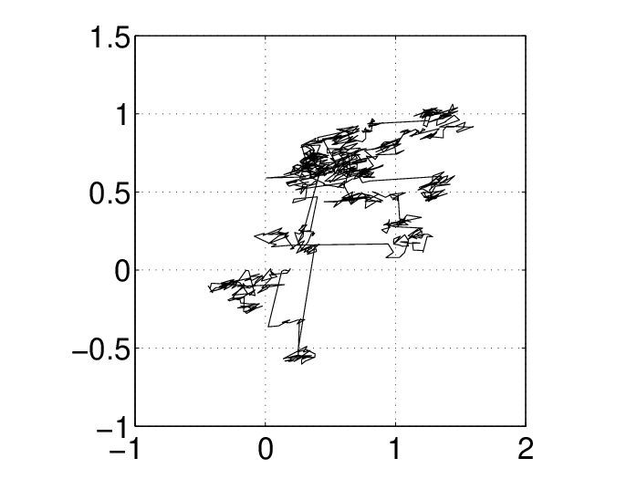
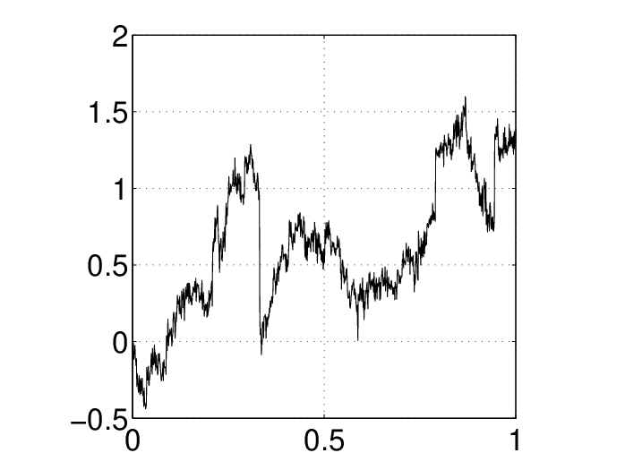
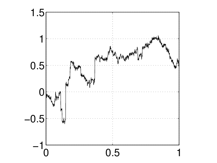
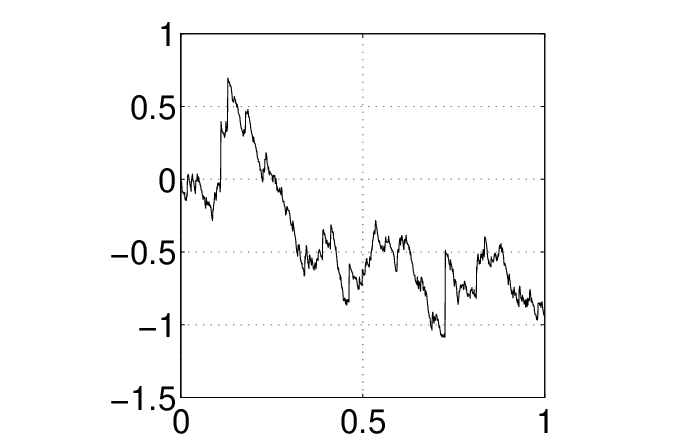
Hence the coordinate marginals are (strictly) stable with index and , respectively. The top right panel in Figure 1 shows a typical sample path of the process, an irregular meandering curve punctuated by occasional large jumps. The top left panel shows the corresponding shot noise part before the Gaussian approximation of the small jumps is added. Since the spectral measure is concentrated on the coordinate axes, the large jumps apparent in the sample path of Figure 1 are all either horizontal or vertical. Pruitt and Taylor [34] showed that the Hausdorff dimension of the sample path is with probability one. Since the spectral measure is concentrated on the coordinate axes, Lemma 2.3 in Meerschaert and Scheffler [26] shows that the coordinates and are independent stable processes. The bottom panels in Figure 1 graph each marginal process. Note that the large jumps occur at different times, reflecting the independence of the marginals. Blumenthal and Getoor [7] showed that the graph of the stable process has Hausdorff dimension .


Example 4.2.
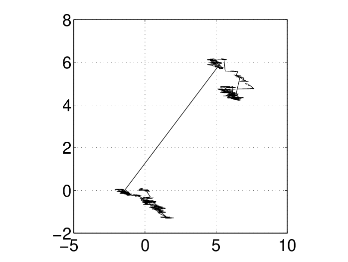
The same exponent is used as in Example 4.1, but now we take the spectral measure . The matrices and turn out to be the same as Example 4.1. The marginals are still stable with index and , but they are no longer symmetric, and we center to zero expectation. From (4.2) we get to compensate the shot noise portion to mean zero. Figure 2 shows a typical sample path and component graphs for this process. Since the spectral measure is concentrated on the positive coordinate axes, the large jumps apparent in the component graphs are all positive.



Example 4.3.
The same exponent is used as in Example 4.1, but now we take the spectral measure to be uniformly distributed on the unit circle: set where are independent standard normal. The matrices and turn out to be the same as Example 4.1. Since , no centering is needed. The marginals are symmetric stable with index and , but they are no longer independent. The top panels in Figure 3 show a typical sample path of the process. Since the spectral measure is uniform, the large jumps apparent in the sample path take a random orientation. Theorem 3.2 in Meerschaert and Xiao [31] shows that the sample path is a random fractal, a set whose Hausdorff and packing dimension are both equal to with probability one. The bottom panels in Figure 3 show the graphs of each marginal process. Note that the large jumps in both marginals are simultaneous, reflecting the dependence.
Example 4.4.
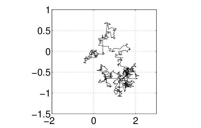
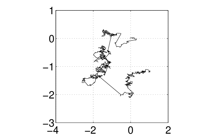
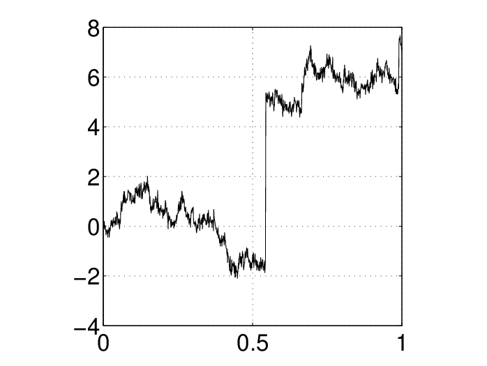
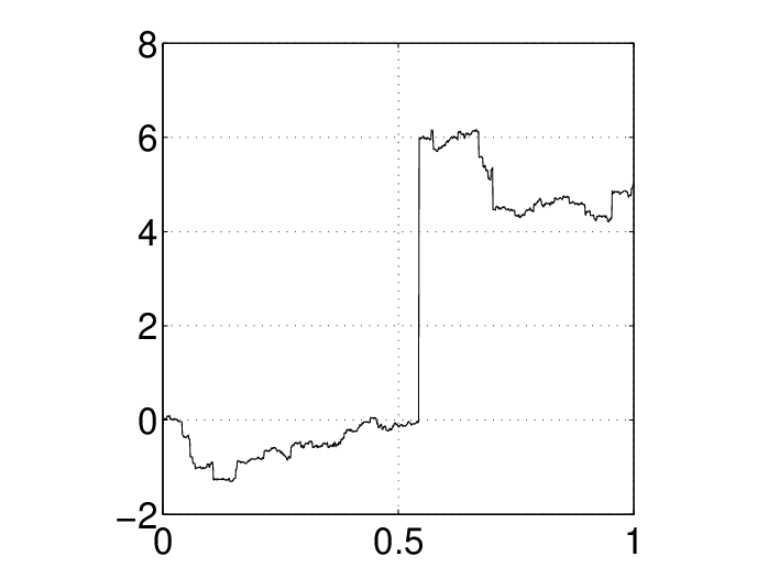
Figure 2 of Zhang et al. [45] represents a model of contaminant transport in fractured rock. Pollution particles travel along fractures in the rock, which form at specific angles due to the geological structure of the rock matrix. An operator stable process represents the path of a pollution particle, with independent skewed stable components in the fracture directions. The skewness derives from the fact that particles jump forward (downstream) when mobilized by water that flows through the fractured rock. The two components of are skewed stable with index on the line with angle measured from the positive axes as usual, and index 1.7 on the line with angle . The two stable laws are independent. The axis represents the overall direction of flow, caused by a differential in hydraulic head (pressure caused by water depth). The exponent has one eigenvalue with associated eigenvector , and another eigenvalue with associated eigenvector . The spectral measure is specified as and , representing the relative fraction of jumps along each fracture direction. In order to compute the matrix power a change of basis is useful. Define the matrix according to so that
and is a diagonal matrix. Then the exponent
From (3.10) we get
Since we can compute and integrate in (3.9) to get the Gaussian covariance matrix whose symmetric square root is given by
To compute the square root, we decompose where , are the eigenvalues of , and the columns of are the corresponding eigenvectors, so that where . From (4.2) we get to compensate the shot noise portion to mean zero. Note that where and are the dual basis vectors. Then each projection is (strictly) stable with index , since
Hence is stable with index and is stable with index . Lemma 2.3 in [26] shows that these two skewed stable marginals of are independent, since the spectral measure is concentrated on the eigenvector coordinate axes . Figure 4 shows a typical sample path, along with the coordinate marginals. Note that the large jumps lie in the directions. The mean zero operator stable process represents particle location in a moving coordinate system, with origin at the center of mass. Hence Figure 4 illustrates the dispersion of a typical pollution particle away from the center of mass of the contaminant plume. Dispersion is the spreading of particles due to variations in velocity, and it is the main cause of plume spreading in ground water hydrology.
Example 4.5.
We simulate an operator stable process whose exponent has a nilpotent part
We choose the spectral measure to place equal masses of at the four points and . Then in (4.2) so that no centering is needed. Here ,
and
Note that where and
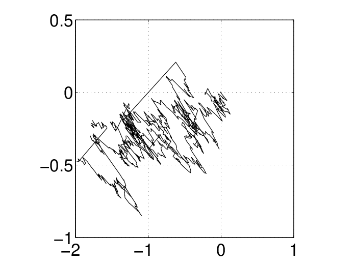
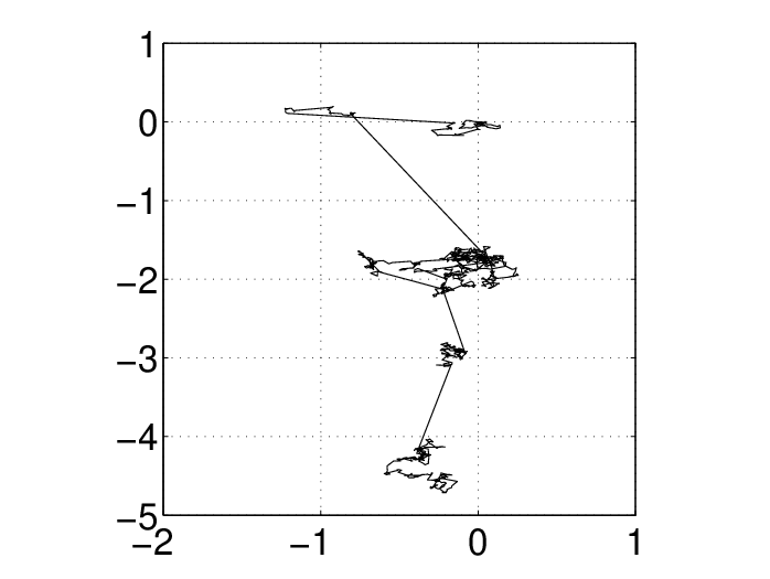
From (4.3) it follows that the second marginal is symmetric stable with index . The first marginal is not stable, but it lies in the domain of attraction of a symmetric stable with index , see [24, Theorem 2]. Figure 5 shows a typical sample path of the process. The large jumps apparent in the sample path of Figure 5 are all of the form where and . Hence they are either vertical, or they lie on the curved orbits . Theorem 3.2 in [31] shows that the sample path is almost surely a random fractal with dimension . Lemma 2.3 in [26] shows that the coordinates and are not independent.
Example 4.6.
We simulate an operator stable process whose exponent
has complex eigenvalues with . We choose the spectral measure to place equal masses of at the four points and , so that in (4.2) and no centering is needed. Here , and
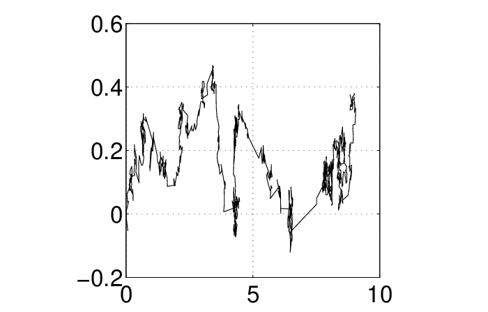
In this case, with , since we can write where the matrix exponential . The coordinate marginals and are not stable, but they are both semistable with index , see [24, Theorem 2]. Lemma 2.3 in [26] shows they are not independent. Figure 6 shows a typical sample path of the process. The large random jumps are of the form where , so that the angle varies along with the length of the jump. The sample path is a fractal with dimension , see [31, Theorem 3.2].

Example 4.7.
Figure 1 in Zhang et al. [45] presents an operator stable model with diagonal exponent
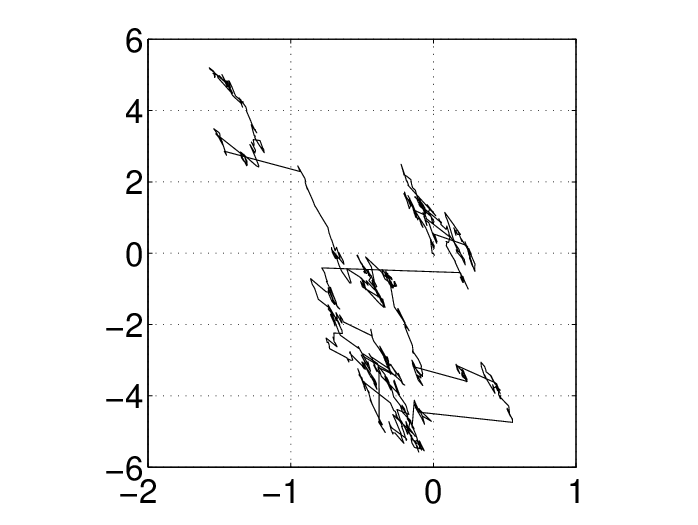
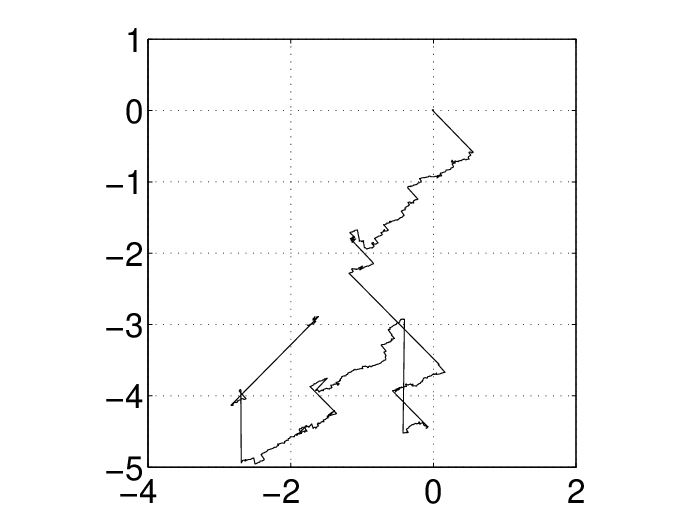
and spectral measure that places masses of 0.3 at , 0.2 at , 0.1 at , and 0.05 at on the unit sphere in the standard Euclidean norm. Large jumps are along the positive -axis, or along the orbits where is a unit vector at , , or , representing displacements of a pollutant particle in an underground aquifer with a mean flow in the positive direction, but some dispersion due to the intervening porous medium. The average plume velocity is so that . Figure 7 depicts the path of a typical particle. Here
and
From (4.2) we compute and, in the simulation code, we first center to mean zero, and then add the mean velocity.
Example 4.8.
This example follows the transport model number 22 for contaminant transport in complex fracture networks from Reeves et al. [37]. The exponent has eigenvectors and at and on the unit circle with eigenvectors and respectively. Writing we get so that
Since we also have
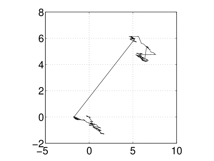
The spectral measure has weights and and 0.2 at . The Lévy measure is concentrated on the two straight line orbits and on the curved orbit . Marginals are stable with index and respectively, but they are not independent, since the spectral measure is not concentrated on the eigenvector axes. The first marginal process is positively skewed, since the projection of the Lévy measure onto the first eigenvector coordinate places all mass on the positive half line. The second marginal is the sum of two independent stable processes, one with positive skewness resulting from the orbit, and one with negative skewness resulting from the projection of the orbit onto the negative axis. As in Example 4.4 we compute and
From (4.2) we compute to correct the shot noise process to mean zero. Figure 8 shows a typical sample path. In this case, the sample path represents the growing deviation of a typical pollution particle from the plume center of mass.

Example 4.9.
This example is an operator stable process whose exponent
The matrix has eigenvalue-eigenvector pairs with , , , and . As in Example 4.4 we compute
We choose the norm (2.8) with . Compute so that the unit sphere is an ellipse, whose major axis is rotated approximately counterclockwise from the direction. Figure 9 shows level sets of this norm. The spectral measure places equal masses of at each point where the unit sphere intersects the coordinate axes: where and . Here , and
The second coordinate is symmetric stable with index , and the projection onto the remaining eigenvector is stable with index . These two stable marginals of are not independent, since the spectral measure is not concentrated on the eigenvector axes. Figure 10 shows a typical sample path for this process. The large jumps of the process are all of the form where or , since we have concentrated the spectral measure at these points. If then, since is an eigenvector of (and hence of ), these jumps will be in the horizontal. The remaining jumps lie along the orbits .
5. Exponents and Symmetries in two dimensions
Section 4 illustrates the wide range of possibilities represented by operator stable Lévy processes in . In this section we will provide a classification of such processes, according to the type of exponent, and the symmetry group. Let be an operator stable Lévy process with exponent , and , as in Section 2. Since the real parts of the eigenvalues of are greater than 1/2, after a change of coordinates, if needed, the exponent assumes one the following Jordan forms
| (5.1) |
where , , and . If , then is a multivariable stable process with index , and all maximal compact subgroups of are admissible as . A genuine operator stable Lévy process is obtained when , . Our first question is, what are possible symmetry groups?
To deal with this question, we need to review some basic facts about subgroups of the orthogonal group on , which can be found, e.g, in [2]. Recall that consists of rotations and reflections,
where
is a rotation counter-clockwise by and is a reflection through the line of angle passing through the origin. The following rules of composition hold: , , , .
The group of rotations is the only infinite proper compact subgroup of . There are also only two kinds of finite subgroups of (modulo the orthogonal conjugacy, see [2, Ch. VII.3]):
- (1)
Cyclic group , ,
- (2)
Dihedral group , .
Notice that , , , and , where
is the reflection with respect to the -axis. We will also need , the group of reflection with respect to the -axis, which is orthogonally conjugate to .
The next result characterizes the possible symmetries of the distribution of in the truly operator stable case where in (5.1) for some . In view of (2.1), the symmetry group do not depend on . Remarkably, once the exponent takes the Jordan form, all symmetries must be orthogonal, not just conjugate to an orthogonal matrix.
Theorem 5.1.
Let be a full operator stable Lévy processes on with an exponent in the Jordan form (5.1), and let . Then the following hold.
- (i)
If , then is either , , , , or .
- (ii)
If , then is either , , or .
- (iii)
If , then is either or .
Proof.
Suppose that has an exponent , , and let be a commuting exponent, see Section 2. If is finite, then , otherwise can be different from . The symmetries defined in (2.3) form a compact subgroup of the centralizer ,
| (5.2) |
First consider finite symmetry groups , so that . If ,
and since is finite (and thus compact),
Thus is either , , , , or , as claimed. If , then
Since is finite (and thus compact),
so that , for some . If ,
and since is finite,
Thus is either or , as claimed.
Now we consider infinite symmetry groups , so that for some symmetric positive definite matrix , see (2.5). From (5.2), commutes with every orthogonal transformation. Thus is a multiple of the identity matrix, which yields
| (5.3) |
Since ,
for some skew symmetric matrix , and so
for some and . This equation eliminates the cases and by comparing the eigenvalues on the left and right hand side. Thus and for some , from which we have
Comparing the determinants of both sides gives . Hence
Since the sets of eigenvalues of both sides of this equation must be the same, or . If then for . A direct verification of this equation reveals that is a multiple of a rotation. (In fact, is a scalar multiple of the identity, since it is also symmetric and positive definite.) Therefore,
as claimed. If , then
or
By the same reason as above, one can verify that is a multiple of rotation. Hence and
This proves that and provided . ∎
Remark 5.2.
Operator stable laws are parameterized by their exponents and spectral measures. Therefore, it is useful to have their symmetries described in terms of these parameters. Recall that denotes the subgroup of rotations of the orthogonal group .
Theorem 5.3.
Let be a full operator stable Lévy process in with exponent and no Gaussian component, and let . Suppose that is given in the Jordan form (5.1) and that the spectral measure is determined by the polar decomposition (2.10) relative to , the Euclidean unit sphere of . Let denote the strict symmetry group of the spectral measure.
- (a)
If , then .
- (b)
If , then either for some , or .
- (c)
If , then .
Proof.
Let be the Lévy measure of . Since does not have a Gaussian part, we have
| (5.4) |
as in (2.11). First we will show that if , and is finite, then
| (5.5) |
Indeed, recall (2.9) and (2.10) for :
Let , being finite. Then by Theorem 5.1 and commutes with . For every , and
because from (5.4). Hence . The proof of the opposite inclusion in (5.5) uses similar arguments and is omitted.
Proof of (a). A direct verification shows that commutes with . Thus by (5.5)
Since by Theorem 5.1, we get (a).
Proof of (b). By Theorem 5.1 for some , or . Suppose that . Since commutes with , by (5.5) we have
Thus .
Suppose . Then for every by (5.4). Since commutes with , by the same line of arguments as in the proof of (5.5). Hence , which implies that is a finite full measure in . Then is a constant multiple of a probability measure, so must be maximal by [25, Theorem 2], and hence .
Proof of (c). It follows from (5.5) because obviously commutes with . ∎
Remark 5.4.
With the help of Theorem 5.3, it is possible to explicitly construct an operator stable process with any given exponent for in the Jordan form (5.1) and any admissible symmetry group. For example, let be concentrated at four points . Choosing masses at these points appropriately, any subgroup of is realized as . By Theorem 5.3, all cases of are realized by this example when and . When , we only get and . To get , , we take concentrated at vertices of a regular -gon inscribed into the unit circle with one vertex at and equal masses at all the vertices. Then , so by Theorem 5.3, . when and is a uniform measure on .
Remark 5.5.
It is interesting to see how much an exponent affects the symmetry. Consider a measure with described in Remark 5.4, with . Then, by Theorem 5.3, when , when , and when . Figure 11 illustrates the diagonal case , in which the Lévy measure in (2.9) is symmetric with respect to reflection about the vertical axis. Here we take and , but any case with appears similar. Figure 12 illustrates the complex case , where the Lévy measure is symmetric with respect to rotations that are a multiple of . Figure 13 illustrates the nilpotent case , and here the Lévy measure has no nontrivial symmetries. All three cases have the same spectral measure, but a different exponent. Hence the spectral measure and the exponent are both important in determining the symmetries.


Remark 5.6.
In order to tie the theoretical results of this section back to the concrete examples in Section 4, we compute the symmetry group for a few interesting cases. For Example 4.1 we have by Theorem 5.3 (a), since the exponent in (5.1), and spectral measure gives equal mass to the four points . The spectral measure in Example 4.3 is uniform on the unit sphere, so that , but the symmetry is of the form in (5.1), so the symmetry group by Theorem 5.3 (a). The construction in Example 4.5 yields . Then since the exponent is nilpotent, by Theorem 5.3 (b). In Example 4.6 we also have , and then by Theorem 5.3 (c). Example 4.7 has since the spectral measure is symmetric with respect to reflection across the -axis: , and , but .
6. Operator self-similar processes
In this section, we discuss more general operator self-similar processes, whose increments need not be independent or stationary. From now on, assume that the operator self-similar process is proper (i.e., for every the smallest hyperplane supporting the distribution of equals ), stochastically continuous, and . Under these assumptions, the real parts of eigenvalues of the exponent are positive [13, Theorem 4]. Denote by the set of linear operators in such that
| (6.1) |
The symmetries of form a compact subgroup of as long as is proper. The symmetry group can be seen as minimal information about a multidimensional stochastic process. Hudson and Mason [13, Theorem 2] proved that
| (6.2) |
where is arbitrary and is the tangent space of at the identity. Maejima [23] showed that one can always find a commuting exponent such that for all .
A shift is included in the symmetry group defined in (2.3) for operator stable Lévy processes, since the definition (2.1) also includes a shift. For operator self-similar processes, the definition (1.1) does not include a shift, so it is natural that the definition (6.1) for the symmetry group of an operator self-similar process does not allow a shift. The following lemma connects with in the operator stable case.
Lemma 6.1.
Let be a strictly operator stable Lévy process with exponent . Suppose that 1 is not an eigenvalue of . Then , where .
Proof.
Since if and only if , we have , so it suffices to show that (see definitions (2.3) and (2.7)). Let , so that and are identically distributed for some . Since the real parts of eigenvalues of all exponents of are the same (see [27, Corollary 7.2.12]), we may take as a commuting exponent. Then, for every we have
Thus for all , and since 1 is not an eigenvalue of , . Hence . The converse inclusion, , is obvious. ∎
Remark 6.2.
Full dimensional operator stable Lévy processes, and proper operator self-similar processes, form two distinct classes. Neither class is contained in the other. Take a spherically symmetric Lévy process on whose marginals are Cauchy. Then is an operator stable Lévy process, but it is not operator self-similar. The process for is operator self-similar but not Lévy. Remark 6.6 provides examples of operator self-similar processes for which none of the one-dimensional distributions are operator stable. The process is a strictly operator stable Lévy process and also a proper operator self-similar process. If we take then but consists of the orthogonal transformations that fix the vector .
Theorem 5.1 and Remark 5.4 showed how to construct an operator stable Lévy process with any admissible symmetry group. The group (and groups conjugated to it) were excluded, since they are not maximal (see Section 1). This raises a question, is it possible to have for some operator self-similar (not Lévy) processes? The answer is affirmative, as shown in the following example.
Example 6.3.
Consider a complex valued process
where , is a uniform random variable on and . Since for any
as a process in ,
is a self-similar with index and . By (6.2), and are exponents of ( with and arbitrary ). If then
which implies . Thus
Consider the process , where is the reflexion with respect to the -axis,
If , then for and we would have
or
This equality written in means
which is impossible since the sum of the first and the fourth random variables on the left hand side is , while on the right hand side is . Hence , which yields .
Remark 6.4.
Example 6.3 is consistent with the result that symmetry groups of probability measures must be maximal [25, Theorem 2], even though is not a maximal subgroup of . This is because, for in , we not only require identically distributed with for a single , but also that is identically distributed with for all finite-dimensional distributions. We say that acts diagonally in this case, and we identify with corresponding element of defined by for . In Example 6.3 the diagonal action of is a maximal subgroup of , see the proof of Theorem 1 in [25].
The exponents of a proper operator self-similar process are related to the symmetry group by (6.2), there always exists a commuting exponent, and the eigenvalues of any exponent all have positive real part. These were the crucial facts used in the proof of Theorem 5.1. Hence we can also characterize the symmetry group of a proper operator self-similar process in in terms of the exponent in Jordan form. The proof is identical to Theorem 5.1, except that here we cannot exclude the case where is conjugate to , as explained in Remark 6.4.
Corollary 6.5.
Remark 6.6.
As a simple extension of the construction in Remark 5.4, we can obtain an operator self-similar process in with any exponent, and any admissible symmetry group. Take as in Remark 5.4 and let where is a self-similar process (time change) with (e.g., take ). Then is operator self-similar with exponent . This, together with Example 6.3, also shows that can take every possible form listed in Corollary 6.5, which therefore provides a complete characterization in of the possible symmetries of an o.s.s. process. An interesting and useful example of a self-similar process with Hurst index , which is not infinitely divisible or even Markovian, is given by the first passage or hitting time of a stable subordinator with . The process has densities that solve the space-time fractional multiscaling diffusion equation
where is the generator of the operator stable semigroup, see for example [28, 29, 45]. This fractional diffusion equation models contaminant transport in heterogeneous porous media, and the process represents the path of a randomly selected contaminant particle. The order of the time fractional derivative controls particle retention (sticking or trapping) while the exponent of the operator stable process codes the anomalous superdiffusion caused by long particle jumps. Also, the inverse process is constant on intervals corresponding to jumps of the stable subordinator , the length of which is determined by the stable index . Note that the time change need not be independent of the outer process [3, 33]. Methods for simulating these non-Markovian subordinated processes have recently been developed by Magdziarz and Weron [20] and Zhang et al. [46].
Remark 6.7.
References
- [1] Søren Asmussen and Jan Rosiński. Approximations of small jumps of Lévy processes with a view towards simulation. J. Appl. Probab., 38(2):482–493, 2001.
- [2] William Barker and Roger Howe. Continuous Symmetry: From Euclid to Klein. American Mathematical Society, 2007.
- [3] P. Becker-Kern, M.M. Meerschaert and H.P. Scheffler (2004) Limit theorems for coupled continuous time random walks. The Annals of Probability 32, No. 1B, 730–756.
- [4] D. Benson, S. Wheatcraft and M. Meerschaert (2000) Application of a fractional advection-dispersion equation. Water Resour. Res. 36, 1403–1412.
- [5] D. Benson, R. Schumer, M. Meerschaert and S. Wheatcraft (2001) Fractional dispersion, Lévy motions, and the MADE tracer tests. Transport in Porous Media 42, 211–240.
- [6] P. Billingsley (1966) Convergence of types in k-space. Z. Wahrsch. Verw. Geb. 5, 175–179.
- [7] R. M. Blumenthal and R. K. Getoor, The dimension of the set of zeros and the graph of a symmetric stable process. Illinois J. Math. 6 1962 308–316.
- [8] S. Cohen, C. Lacaux, and M. Ledoux. (2008) A general framework for simulation of fractional fields. Stochastic Process. Appl. 118(9), 1489–1517.
- [9] S. Cohen and Rosiński. Gaussian approximation of multivariate Lévy processes with applications to simulation of tempered stable processes. Bernoulli, 13(1):195–210, 2007.
- [10] Rama Cont and Peter Tankov. Financial modelling with jump processes. Chapman & Hall/CRC, Boca Raton, Florida, 2004.
- [11] P. Embrechts and M. Maejima (2002) Self-similar Processes. Princeton University Press.
- [12] Franklin A. Graybill. Matrices with applications in statistics. Wadsworth Statistics/Probability Series. Wadsworth Advanced Books and Software, Belmont, Calif., second edition, 1983.
- [13] William N. Hudson and J. David Mason. Operator-self-similar processes in a finite-dimensional space. Trans. Amer. Math. Soc., 273(1):281–297, 1982.
- [14] H.E. Hurst, R.P. Black, and Y.M. Simaika (1965) Long-term Storage: An Experimental Study, Constable, London.
- [15] Aleksander Janicki and Aleksander Weron. Simulation and Chaotic Behavior of -Stable Stochastic Processes. Monographs and Textbooks in Pure and Applied Mathematics. Marcel Dekker Inc. New York, 1994.
- [16] Zbigniew J. Jurek and J. David Mason. Operator-Limit Distributions in Probability Theory. Wiley Series in Probability and Mathematical Statistics. John Wiley & Sons Inc., New York, 1993.
- [17] Olav Kallenberg. Foundations of Modern Probability. Probability and its Applications (New York). Springer-Verlag, New York, second edition, 2002.
- [18] Peter E. Kloeden and Eckhard Platen. Numerical solution of stochastic differential equations. Applications of Mathematics. Springer-Verlag, New York, 1992.
- [19] Céline Lacaux. Series representation and simulation of multifractional Lévy motions. Adv. in Appl. Probab., 36(1):171–197, 2004.
- [20] Magdziarz, M., and A. Weron, Competition between subdiffusion and Lévy flights: A Monte Carlo approach, Phys. Rev. E, 75, 056702, 2007.
- [21] Maejima, M. and J. D. Mason (1994) Operator-self-similar stable processes. Stoch. Proc. Appl. 54, 139–163.
- [22] Makoto Maejima. Operator-stable processes and operator fractional stable motions. Probab. Math. Statist., 15:449–460, 1995. Dedicated to the memory of Jerzy Neyman.
- [23] Makoto Maejima. Norming operators for operator-self-similar processes. Trends Math., Birkhäuser, Boston 287–295, 1998.
- [24] M.M. Meerschaert and H.P. Scheffler, One dimensional marginals of operator stable laws and their domains of attraction, Publ. Math. Debrecen, 55(3–4), 487–499, 1999.
- [25] Mark M. Meerschaert and J. A. Veeh. Symmetry groups in -space. Statistics & Probability Letters 22:1–6, 1995.
- [26] Mark M. Meerschaert and Hans-Peter Scheffler. Sample cross-correlations for moving averages with regularly varying tails. Journal of Time Series Analysis, 22(4):481–492, 2001.
- [27] Mark M. Meerschaert and Hans-Peter Scheffler. Limit Distributions for Sums of Independent Random Vectors: Heavy Tails in Theory and Practice. Wiley Series in Probability and Statistics. John Wiley & Sons Inc., New York, 2001.
- [28] Meerschaert, M., D. Benson and B. Baeumer (2001) Operator Lévy motion and multiscaling anomalous diffusion. Phys. Rev. E 63, 1112–1117.
- [29] M.M. Meerschaert, D.A. Benson, H.P. Scheffler and B. Baeumer (2002) Stochastic solution of space-time fractional diffusion equations. Phys. Rev. E 65, 1103–1106.
- [30] M.M. Meerschaert and H.P. Scheffler, Portfolio modeling with heavy tailed random vectors. Handbook of Heavy-Tailed Distributions in Finance, 595–640, S. T. Rachev, Ed., Elsevier North-Holland, New York, 2003.
- [31] Mark M. Meerschaert and Yimin Xiao. Dimension results for sample paths of operator stable Levy processes. Stochastic Processes and Their Applications, 115(1):55–75, 2005.
- [32] M.M. Meerschaert, E. Scalas, Coupled continuous time random walks in finance. Physica A: Statistical Mechanics and Its Applications, 370, 114–118, 2006.
- [33] Meerschaert, M.M. and H.-P. Scheffler (2008) Triangular array limits for continuous time random walks. Stoch. Proc. Appl., 118, 1606–1633.
- [34] W.E. Pruitt and S.J. Taylor (1969) Sample path properties of processes with stable components. Z. Wahrsch. verw. Geb. 12, 267–289.
- [35] Rachev, S. and S. Mittnik (2000) Stable Paretian Models in Finance, Wiley, Chichester.
- [36] B.S. Rajput and J. Rosiński. Spectral representations of infinitely divisible processes. Probab. Th. Rel. Fields, 82: 451–487, 1989.
- [37] D.M. Reeves, D.A. Benson, M.M. Meerschaert, H.P. Scheffler, Transport of Conservative Solutes in Simulated Fracture Networks 2. Ensemble Solute Transport and the Correspondence to Operator-Stable Limit Distributions, Water Resources Research, 44 (2008), W05410.
- [38] J. Rosiński. On series representations of infinitely divisible random vectors. Ann. Probab., 82: 405–430, 1990.
- [39] Jan Rosiński. Series representations of Lévy processes from the perspective of point processes. In Lévy processes, pages 401–415. Birkhäuser Boston, Boston, MA, 2001.
- [40] Jan Rosiński. Tempering stable processes. Bernoulli, 13:195-210, 2007.
- [41] Ken-Iti Sato. Strictly operator-stable distributions. Journal of Multivariate Analysis, 22:278–285, 1987.
- [42] Ken-iti Sato. Lévy Processes and Infinitely Divisible Distributions, volume 68 of Cambridge Studies in Advanced Mathematics. Cambridge University Press, Cambridge, 1999. Translated from the 1990 Japanese original, Revised by the author.
- [43] E. Scalas, R. Gorenflo, F. Mainardi, and M.M. Meerschaert, Speculative option valuation and the fractional diffusion equation, Fractional Derivatives and Their Applications, 265–274, A. Le Mehauté, J. A. Tenreiro Machado, J. C. Trigeassou and J. Sabatier, Eds. (2005), Ubooks, Germany.
- [44] Oleg Sheluhin, Sergey Smolskiy, Andrew Osin, Self-Similar Processes in Telecommunications, Wiley, New York, 2007.
- [45] Y. Zhang, D.A. Benson, M.M. Meerschaert, E. M. LaBolle, and H.P. Scheffler. Random walk approximation of fractional-order multiscaling anomalous diffusion. Physical Review E, 74(2):6706–6715, 2006.
- [46] Y. Zhang, M.M. Meerschaert, B. Baeumer (2008) Particle tracking for time-fractional diffusion, Physical Review E, 78(3), 036705.