跳到论文正文
W Papers独立论文阅读器 arXiv:0912.4686 论文正文 计算阅读时间 · 0%
引用这篇论文根据当前论文元数据生成,正式投稿前建议核对。


License: arXiv.org perpetual non-exclusive license
arXiv:0912.4686v1 [math.ST] 23 Dec 2009

Robust estimation of the scale and of the autocovariance function of Gaussian short and long-range dependent processes

C. Lévy-Leduc Address: CNRS/LTCI/Telecom ParisTech - 46, rue Barrault, 75634 Paris Cédex 13, France. Email address: celine.levy-leduc@telecom-paristech.fr , H. Boistard Address: GREMAQ, Université Toulouse 1 - Manufacture des Tabacs, bât. F, aile J.J. Laffont - 21 allée de Brienne - 31000 Toulouse Email address: helene@boistard.fr , E. Moulines Address: Institut Telecom/Telecom ParisTech - 46, rue Barrault, 75634 Paris Cédex 13, France. Email address: eric.moulines@telecom-paristech.fr , M. S. Taqqu Address: Department of Mathematics, Boston University, 111 Cumington Street, Boston, MA 02215, USA Email address: murad@bu.edu and V. A. Reisen Address: Departamento de Estatística, Universidade Federal do Espírito Santo, Vitória/ES, Brazil Email address: valderio@cce.ufes.br
Date: August 24, 2026
Abstract.

A desirable property of an autocovariance estimator is to be robust to the presence of additive outliers. It is well-known that the sample autocovariance, being based on moments, does not have this property. Hence, the use of an autocovariance estimator which is robust to additive outliers can be very useful for time-series modeling. In this paper, the asymptotic properties of the robust scale and autocovariance estimators proposed by Rousseeuw and Croux (1993) and Ma and Genton (2000) are established for Gaussian processes, with either short-range or long-range dependence. It is shown in the short-range dependence setting that this robust estimator is asymptotically normal at the rate n\sqrt{n}, where nn is the number of observations. An explicit expression of the asymptotic variance is also given and compared to the asymptotic variance of the classical autocovariance estimator. In the long-range dependence setting, the limiting distribution displays the same behavior than that of the classical autocovariance estimator, with a Gaussian limit and rate n\sqrt{n} when the Hurst parameter HH is less 3/43/4 and with a non-Gaussian limit (belonging to the second Wiener chaos) with rate depending on the Hurst parameter when H∈(3/4,1)H\in(3/4,1). Some Monte-Carlo experiments are presented to illustrate our claims and the Nile River data is analyzed as an application. The theoretical results and the empirical evidence strongly suggest using the robust estimators as an alternative to estimate the dependence structure of Gaussian processes.

Key words and phrases: 
autocovariance function, long-memory, robustness, influence function, scale estimator, Hadamard differentiability, functional Delta method.

1. Introduction

The autocovariance function of a stationary process plays a key role in time series analysis. However, it is well known that the classical sample autocovariance function is very sensitive to the presence of additive outliers in the data. A small fraction of additive outliers, in some cases even a single outlier, can affect the classical autocovariance estimate making it virtually useless; see for instance Deutsch et al. (1990) Chan (1992), Chan (1995) (Maronna et al., 2006, Chapter 8) and the references therein. Since additive outliers are quite common in practice, the definition of an autocovariance estimator which is robust to the presence of additive outliers is an important task.

Ma and Genton (2000) proposed a robust estimator of the autocovariance function and discussed its performance on synthetic and real data sets. This estimator has later been used by Fajardo et al. (2009) to derive robust estimators for ARMA and ARFIMA models.

The autocovariance estimator proposed by Ma and Genton (2000) is based on a method due to Gnanadesikan and Kettenring (1972), which consists in estimating the covariance of the random variables XX and X′X^{\prime} by comparing the scale of two appropriately chosen linear combinations of these variables; more precisely, if aa and bb are non-zero, then

Cov⁡(X,X′)=14​a​b​{Var(a​X+b​X′)−Var(a​X−b​X′)}.\mathrm{Cov}(X,X^{\prime})=\frac{1}{4ab}\left\{\mathop{\rm Var}\nolimits(aX+bX^{\prime})-\mathop{\rm Var}\nolimits(aX-bX^{\prime})\right\}\;. (1)

Assume that S\mathrm{S} is a robust scale functional; we write for short S⁡(X)=S⁡(FX)\mathrm{S}(X)=\mathrm{S}(F_{X}), where FXF_{X} is the c.d.f of XX and assume that S\mathrm{S} is affine equivariant in the sense that S⁡(a​X+b)=|a|​S​(X)\mathrm{S}(aX+b)=|a|\mathrm{S}(X). Following Huber (1981), if we replace in the above expression Var(⋅)\mathop{\rm Var}\nolimits(\cdot) by S2​(⋅)\mathrm{S}^{2}(\cdot), then (1) is turned into the definition of a robust alternative to the covariance

CS​(X,X′)=14​a​b​{S2​(a​X+b​X′)−S2​(a​X−b​X′)}.\mathrm{C}_{\mathrm{S}}(X,X^{\prime})=\frac{1}{4ab}\left\{\mathrm{S}^{2}(aX+bX^{\prime})-\mathrm{S}^{2}(aX-bX^{\prime})\right\}\;. (2)

The constants aa and bb can be chosen arbitrarily. If XX and X′X^{\prime} have the same scale (e.g. the same marginal distribution), one could simply take a=b=1a=b=1. Gnanadesikan and Kettenring (1972) suggest to take aa and bb proportional to the inverse of S⁡(X)\mathrm{S}(X) and S⁡(X′)\mathrm{S}(X^{\prime}), respectively in order to standardize XX and X′X^{\prime}. As explained in Huber (1981), if S\mathrm{S} is standardized such that S⁡(X)=1\mathrm{S}(X)=1 in the case where XX is standard Gaussian, then, provided that (X,X′)(X,X^{\prime}) is bivariate normal,

CS​(X,X′)=Cov⁡(X,X′).\mathrm{C}_{\mathrm{S}}(X,X^{\prime})=\mathrm{Cov}(X,X^{\prime})\;. (3)

In this case indeed, a​X+b​X′aX+bX^{\prime} and a​X−b​X′aX-bX^{\prime} are Gaussian random variables with variance σ±2=a2​Var(X)±2​a​b​Cov​(X,X′)+b2​Var(X′)\sigma^{2}_{\pm}=a^{2}\mathop{\rm Var}\nolimits(X)\pm 2ab\mathrm{Cov}(X,X^{\prime})+b^{2}\mathop{\rm Var}\nolimits(X^{\prime}), and so, if Y∼𝒩⁡(0,1)Y\sim\mathcal{N}(0,1), then S⁡(a​X±b​X′)=S⁡(σ±​Y)=σ±​S​(Y)=σ±S(aX\pm bX^{\prime})=S(\sigma_{\pm}Y)=\sigma_{\pm}S(Y)=\sigma_{\pm} and S2​(a​X+b​X′)−S2​(a​X−b​X′)=σ+2−σ−2=4​a​b​Cov​(X,X′)S^{2}(aX+bX^{\prime})-S^{2}(aX-bX^{\prime})=\sigma^{2}_{+}-\sigma^{2}_{-}=4ab\mathrm{Cov}(X,X^{\prime}) yielding CS​(X,X′)=Cov⁡(X,X′).C_{S}(X,X^{\prime})=\mathrm{Cov}(X,X^{\prime}).

Ma and Genton (2000) suggested to use for S\mathrm{S} the robust scale estimator introduced in Rousseeuw and Croux (1993). This scale estimator is based on the Grassberger-Procaccia correlation integral, defined as

r↦U(r,FX)=∬𝟙{|x−x′|≤r}dFX(x)dFX(x′),r\mapsto U(r,F_{X})=\iint\mathbbm{1}_{\{|x-x^{\prime}|\leq r\}}\mathrm{d}F_{X}(x)\mathrm{d}F_{X}(x^{\prime})\;, (4)

which measures the probability that two independent copies XX and X′X^{\prime} distributed according to FXF_{X} fall at a distance smaller than rr. The robust scale estimator introduced in (Rousseeuw and Croux, 1993, p. 1277) defines the scale Q⁡(FX)Q(F_{X}) of a c.d.f. FXF_{X} as being proportional to the first quartile of r↦U⁡(r,FX)r\mapsto U(r,F_{X}), namely,

Q⁡(FX)=c⁡(FX)​inf{r≥0,U⁡(r,FX)≥1/4},Q(F_{X})=c(F_{X})\inf\left\{r\geq 0,U(r,F_{X})\geq 1/4\right\}\;, (5)

where c⁡(FX)c(F_{X}) is a constant depending only on the shape of the c.d.f. FXF_{X}. We see immediately that Q⁡(FX)Q(F_{X}) is affine invariant, in the sense that transforming XX into a​X+baX+b, will multiply Q⁡(FX)Q(F_{X}) by |a||a| . This scale can be seen as an analog of the Gini average difference estimator n−1​(n−1)−1​∑1≤i≠j≤n|Xi−Xj|n^{-1}(n-1)^{-1}\sum_{1\leq i\neq j\leq n}|X_{i}-X_{j}|, where the average is replaced by a quantile. It is worth noting that instead of measuring how far away the observations are from a central value, Q⁡(FX)Q(F_{X}) computes a typical distance between two independent copies of the random variable XX, which leads to a reasonable estimation of the scale even when the c.d.f. FXF_{X} is not symmetric.

The constant c⁡(FX)c(F_{X}) in (5) is there to ensure consistency. In the sequel, the c.d.f. FXF_{X} is assumed to belong to the Gaussian location-scale family

{Φμ,σ(⋅)=Φ((⋅−μ)/σ),μ∈ℝ,σ∈ℝ+∗},\{\Phi_{\mu,\sigma}(\cdot)=\Phi((\cdot-\mu)/\sigma),\ \mu\in\mathbb{R},\sigma\in\mathbb{R}^{*}_{+}\}\;, (6)

where Φ\Phi is the c.d.f. of a standard Gaussian random variable. The reason we focus on the Gaussian family is that if we want to use QQ as the scale SS in (2), we will need to compute c⁡(Fa​X+b​X′)c(F_{aX+bX^{\prime}}) and c⁡(Fa​X−b​X′)c(F_{aX-bX^{\prime}}). This is easily done when (X,X′)(X,X^{\prime}) is a Gaussian vector. Indeed, in view of (3), one has

Cov⁡(X,X′)=14​[Q2​(FX+X′)−Q2​(FX−X′)],\mathrm{Cov}(X,X^{\prime})=\frac{1}{4}\left[Q^{2}(F_{X+X^{\prime}})-Q^{2}(F_{X-X^{\prime}})\right]\;, (7)

and in particular, since by (4) and (5), Q2​(F2​X)=(2​Q​(FX))2Q^{2}(F_{2X})=(2Q(F_{X}))^{2},

Var(X)=Q2​(FX).\mathop{\rm Var}\nolimits(X)=Q^{2}(F_{X})\;. (8)

When FX=Φμ,σF_{X}=\Phi_{\mu,\sigma} we can then obtain the constant c⁡(Φμ,σ)c(\Phi_{\mu,\sigma}) in (5) explicitly as noted by Rousseeuw and Croux (1993). Since Q⁡(Φμ,σ)=σQ(\Phi_{\mu,\sigma})=\sigma, (5) becomes

σ=Q⁡(Φμ,σ)=c⁡(Φμ,σ)​σ​r0\sigma=Q(\Phi_{\mu,\sigma})=c(\Phi_{\mu,\sigma})\sigma r_{0} (9)

where r0r_{0} is such that, in (4), U⁡(r0,Φ)=1/4U(r_{0},\Phi)=1/4. Hence for all (μ,σ)∈ℝ×ℝ+∗(\mu,\sigma)\in\mathbb{R}\times\mathbb{R}_{+}^{*},

c⁡(Φμ,σ)=c⁡(Φ)=1/r0=1/(2​Φ−1​(5/8))=2.21914.c(\Phi_{\mu,\sigma})=c(\Phi)=1/r_{0}=1/(\sqrt{2}\Phi^{-1}(5/8))=2.21914\;. (10)

Let (Xi)i≥1(X_{i})_{i\geq 1} be a stationary Gaussian process. Given the observations X1:n=(X1,…,Xn)X_{1:n}=(X_{1},\dots,X_{n}), the c.d.f. of the observations may be estimated using the empirical c.d.f. r↦Fn(r)=n−1∑i=1n𝟙{Xi≤r}r\mapsto F_{n}(r)=n^{-1}\sum_{i=1}^{n}\mathbbm{1}_{\{X_{i}\leq r\}}. Plugging FnF_{n} into (5) leads to the following robust scale estimator

Qn(X1:n,Φ)=c(Φ){|Xi−Xj|; 1≤i,j≤n}(kn),\mathrm{Q}_{n}\left(X_{1:n},\Phi\right)=c(\Phi)\{|X_{i}-X_{j}|;\ 1\leq i,j\leq n\}_{(k_{n})}\;, (11)

where kn=⌊n2/4⌋k_{n}=\lfloor n^{2}/4\rfloor. That is, up to the multiplicative constant c⁡(Φ)c(\Phi), Qn(X1:n,Φ)\mathrm{Q}_{n}\left(X_{1:n},\Phi\right) is the knk_{n}th order statistics of the n2n^{2} distances |Xi−Xj||X_{i}-X_{j}| between all the pairs of observations.

As mentioned by Rousseeuw and Croux (1993), Qn(X1:n,Φ)\mathrm{Q}_{n}\left(X_{1:n},\Phi\right) has several appealing properties: it has a simple and explicit formula with an intuitive meaning; it has the highest possible breakdown point (50%\%); in addition, the associated influence function (see below) is bounded. For a definition of these quantities, which are classical in robust statistics, see for instance Huber (1981). The scale estimator of Rousseeuw and Croux is also attractive because it can be implemented very efficiently; it can be computed with a time-complexity of order O⁡(n​log⁡n)O(n\log n) and with a storage scaling linearly O⁡(n)O(n); see Croux and Rousseeuw (1992) for implementation details.

Using the robust scale estimator Qn​(⋅,Φ)\mathrm{Q}_{n}\left(\cdot,\Phi\right) in (11) and the identity (2) with a=b=1a=b=1, the robust autocovariance estimator of

γ⁡(h)=Cov⁡(X1,Xh+1)=14​{Var(X1+Xh+1)−Var(X1−Xh+1)}\gamma(h)=\mathrm{Cov}(X_{1},X_{h+1})=\frac{1}{4}\{\mathop{\rm Var}\nolimits(X_{1}+X_{h+1})-\mathop{\rm Var}\nolimits(X_{1}-X_{h+1})\}

is

γ^Q(h,X1:n,Φ)=14{Qn−h2(X1:n−h+Xh+1:n,Φ)−Qn−h2(X1:n−h−Xh+1:n,Φ)}.\widehat{\gamma}_{Q}(h,X_{1:n},\Phi)=\frac{1}{4}\left\{\mathrm{Q}^{2}_{n-h}\left(X_{1:n-h}+X_{h+1:n},\Phi\right)-\mathrm{Q}^{2}_{n-h}\left(X_{1:n-h}-X_{h+1:n},\Phi\right)\right\}\;\;. (12)

Thus, in the sample version (12), the random variable X1±Xh+1X_{1}\pm X_{h+1} is replaced by the vector X1:n−h±Xh+1:nX_{1:n-h}\pm X_{h+1:n} of length n−hn-h.

In this paper, we establish the asymptotic properties of Qn(X1:n,Φ)\mathrm{Q}_{n}\left(X_{1:n},\Phi\right) and the corresponding robust autocovariance estimator γ^Q(h,X1:n,Φ)\widehat{\gamma}_{Q}(h,X_{1:n},\Phi) for Gaussian processes displaying both short-range and long-range dependence. We say that the process is short-range dependent if the autocovariance function {γ⁡(k)}k∈ℤ\{\gamma(k)\}_{k\in\mathbb{Z}} is absolutely summable, ∑k∈ℤ|γ⁡(k)|<∞\sum_{k\in\mathbb{Z}}|\gamma(k)|<\infty. We say that it is long-range dependent if the autocovariance function is regularly varying at infinity with exponent DD, γ⁡(k)=k−D​L​(k)\gamma(k)=k^{-D}L(k) with 0<D<10<D<1 and LL is a slowly varying function, i.e. limk→∞L⁡(a​k)/L⁡(k)\lim_{k\to\infty}L(ak)/L(k) for any a>0a>0, and is positive for large enough kk. The exponent DD is related to the so-called Hurst coefficient by the relation H=1−D/2H=1-D/2. See, for more details, (Doukhan et al., 2003, p. 5–38).

The limiting distributions of these estimators are obtained by using the functional delta method; see van der Vaart (1998). In the short memory case, the results stems directly from the weak invariance principle satisfied by the empirical process FnF_{n} under mild technical assumptions. The rate of convergence of the robust covariance estimator is n\sqrt{n} and the limiting distribution is Gaussian; an explicit expression of the asymptotic variance is given in Theorem 4.

In the long memory case, the situation is more involved. When D≥1/2D\geq 1/2 (or H≤3/4H\leq 3/4), the rate of convergence is still n\sqrt{n}, the limiting distribution is Gaussian and the asymptotic variance of the covariance estimator is the same as in the short-memory case. When 0<D<1/20<D<1/2, the rate of convergence becomes equal to nD/L~​(n)n^{D}/\widetilde{L}(n) where L~\widetilde{L} is a slowly varying function defined in (38); the limiting distribution is non-Gaussian and belongs to the second Wiener Chaos; see Theorem 8. We prove that these rates are identical to the ones of the classical autocovariance estimators.

The study of the asymptotic distribution of the empirical process is not enough to derive these results. It is necessary to use results on the empirical version of the correlation integral which requires extensions of the results derived for UU-processes under short-range dependence conditions by Borovkova et al. (2001). For this part, we use novel results on UU-processes of long-memory time-series that are developed in a companion paper Lévy-Leduc et al. (2009).

The outline of the paper is as follows. In Section 2, the limiting distributions of the robust scale estimator Qn(X1:n,Φ)\mathrm{Q}_{n}\left(X_{1:n},\Phi\right) in the Gaussian short-range and long-range dependence settings are proved. From these results, the asymptotic distribution of γ^Q(h,X1:n,Φ)\widehat{\gamma}_{Q}(h,X_{1:n},\Phi) is derived. In Section 3, some Monte-Carlo experiments are presented in order to support our theoretical claims. The Nile River data is studied as an application in Section 4. Section 5 is dedicated to the asymptotic properties of UU-processes which are useful to establish the results of Section 2 in the long-range case. Sections 6 and 7 detail the proofs of the theoretical results stated in Section 2. Some concluding remarks are provided in Section 8.

Notation. For an interval II in the extended real line [−∞,∞][-\infty,\infty], we denote by 𝖣⁡(I)\mathsf{D}(I) the set of all functions z:I→ℝz:I\to\mathbb{R} that are right-continuous and whose limits from the left exist everywhere on II. We always equip 𝖣⁡(I)\mathsf{D}(I) with the uniform norm, denoted by ‖⋅‖∞\left\|\cdot\right\|_{\infty}. We denote by ℳ⁡([−∞,∞])\mathcal{M}([-\infty,\infty]) the set of cumulative distribution functions on [−∞,∞][-\infty,\infty] equipped with the topology of uniform convergence. For U∈𝖣⁡(I)U\in\mathsf{D}(I), let U−1U^{-1} denote its generalized inverse, U−1​(η)=inf{r∈I,U⁡(r)≥η}U^{-1}(\eta)=\inf\{r\in I,U(r)\geq\eta\}.

The convergence in distribution in (𝖣⁡([0,∞]),‖⋅‖∞)\left(\mathsf{D}([0,\infty]),\left\|\cdot\right\|_{\infty}\right) is meant with respect to the σ\sigma-algebra generated by the set of open balls. We denote by ⟶d\stackrel{{\scriptstyle d}}{{\longrightarrow}} the convergence in distribution.

We denote by Φ\Phi the c.d.f of the standard Gaussian random variable and by ϕ\phi the corresponding density function.

2. Theoretical results

Define the following mappings:

T1:\displaystyle T_{1}: ℳ⁡([−∞,∞])\displaystyle\mathcal{M}([-\infty,\infty]) →𝖣⁡([0,∞])\displaystyle\to\mathsf{D}([0,\infty]) (13)
F\displaystyle F ↦{r↦∫ℝ∫ℝ𝟙{|x−y|≤r}dF(x)dF(y)},\displaystyle\mapsto\left\{r\mapsto\int_{\mathbb{R}}\int_{\mathbb{R}}\mathbbm{1}_{\{|x-y|\leq r\}}\mathrm{d}F(x)\mathrm{d}F(y)\right\}\;,
T2:\displaystyle T_{2}: 𝖣⁡([0,∞])\displaystyle\mathsf{D}([0,\infty]) →ℝ\displaystyle\to\mathbb{R} (14)
U\displaystyle U ↦U−1​(1/4).\displaystyle\mapsto U^{-1}(1/4)\;.

and

T0=T2∘T1:\displaystyle T_{0}=T_{2}\circ T_{1}: OPENℳ⁡([−∞,∞]))\displaystyle\mathcal{M}([-\infty,\infty])) →ℝ\displaystyle\to\mathbb{R} (15)
F\displaystyle F ↦U−1​(1/4).\displaystyle\mapsto U^{-1}(1/4)\;. (16)

Then, the scale estimator Qn(X1:n,Φ)\mathrm{Q}_{n}\left(X_{1:n},\Phi\right) introduced in (11) may be expressed as

Qn(X1:n,Φ)=c(Φ)T0(Fn),\mathrm{Q}_{n}\left(X_{1:n},\Phi\right)=c(\Phi)T_{0}(F_{n})\;, (17)

where FnF_{n} is the empirical c.d.f. based on X1:nX_{1:n}.

2.1. Short-range dependence setting

2.1.1. Properties of the scale estimator

The following lemma gives an asymptotic expansion for Qn(X1:n,Φ)\mathrm{Q}_{n}\left(X_{1:n},\Phi\right), which is used for deriving a Central Limit Theorem (Theorem 2). It supposes that the empirical c.d.f. FnF_{n}, adequately normalized, converges.

Lemma 1.

Let (Xi)i≥1(X_{i})_{i\geq 1} be a stationary Gaussian process. Assume that there exists a non-decreasing sequence (an)(a_{n}) such that an​(Fn−Φμ,σ)a_{n}(F_{n}-\Phi_{\mu,\sigma}) converges weakly in (𝖣⁡([0,∞]),‖⋅‖∞)\left(\mathsf{D}([0,\infty]),\left\|\cdot\right\|_{\infty}\right). Then, Qn(X1:n,Φ)\mathrm{Q}_{n}\left(X_{1:n},\Phi\right) defined by (11) has the following asymptotic expansion:

an(Qn(X1:n,Φ)−σ)=ann∑i=1nIF(Xi,Q,Φμ,σ)+oP(1),a_{n}\left(\mathrm{Q}_{n}\left(X_{1:n},\Phi\right)-\sigma\right)=\frac{a_{n}}{n}\sum_{i=1}^{n}\mathrm{IF}(X_{i},Q,\Phi_{\mu,\sigma})+o_{P}(1)\;, (18)

where, for all xx in ℝ\mathbb{R},

IF⁡(x,Q,Φμ,σ)=σ​IF​((x−μ)/σ,Q,Φ),\mathrm{IF}(x,Q,\Phi_{\mu,\sigma})=\sigma\mathrm{IF}((x-\mu)/\sigma,Q,\Phi)\;, (19)

and

IF⁡(x,Q,Φ)=c⁡(Φ)​(1/4−Φ⁡(x+1/c⁡(Φ))+Φ⁡(x−1/c⁡(Φ))∫ℝϕ⁡(y)​ϕ​(y+1/c⁡(Φ))​𝑑y).\mathrm{IF}(x,Q,\Phi)=c(\Phi)\left(\frac{1/4-\Phi(x+1/c(\Phi))+\Phi(x-1/c(\Phi))}{\int_{\mathbb{R}}\phi(y)\phi(y+1/c(\Phi))\mathrm{d}y}\right)\;. (20)

The proof of Lemma 1 is given in Section 6.

Remark 1.

Note that IF⁡(x,Q,Φ)\mathrm{IF}(x,Q,\Phi) has the same expression as the influence function of the functional QQ evaluated at the c.d.f. Φ\Phi given by (Rousseeuw and Croux, 1993, p. 1277) and (Ma and Genton, 2000, p. 675). As is well-known from (Huber, 1981, p. 13), the influence function x↦IF⁡(x,T,F)x\mapsto\mathrm{IF}(x,T,F) is defined for a functional TT at a distribution FF at point xx as the limit

IF⁡(x,T,F)=limε→0+ε−1​{T⁡(F+ε⁡(δx−F))−T⁡(F)},\mathrm{IF}(x,T,F)=\lim_{\varepsilon\to 0+}\varepsilon^{-1}\{T(F+\varepsilon(\delta_{x}-F))-T(F)\}\;,

where δx\delta_{x} is the Dirac distribution at xx. Influence functions are a classical tool in robust statistics used to understand the effect of a small contamination at the point xx on the estimator.

We focus here on the case where the process (Xi)i≥1(X_{i})_{i\geq 1} satisfies the following assumption:

  • (A1)

    (Xi)i≥1(X_{i})_{i\geq 1} is a stationary mean-zero Gaussian process with autocovariance sequence γ⁡(k)=𝔼⁡(X1​Xk+1)\gamma(k)=\mathbb{E}(X_{1}X_{k+1}) satisfying:

    ∑k≥1|γ⁡(k)|<∞.\sum_{k\geq 1}|\gamma(k)|<\infty\;.

To state the results, we must first define the Hermite rank of the influence function x↦IF⁡(x,Q,Φ)x\mapsto\mathrm{IF}(x,Q,\Phi). Let {Hk}\{H_{k}\} denote the Hermite polynomials having leading coefficient equal to one. These are H0​(x)=1H_{0}(x)=1, H1​(x)=xH_{1}(x)=x, H2​(x)=x2−1H_{2}(x)=x^{2}-1, ⋯\cdots. Let ff be a function such that ∫f2​(z)​𝑑Φ​(z)<∞\int f^{2}(z)\mathrm{d}\Phi(z)<\infty. The expansion of ff in Hermite polynomials is given by

f⁡(z)=∑q=τ⁡(f)∞αq​(f)q!​Hq​(z),f(z)=\sum_{q=\tau(f)}^{\infty}\frac{\alpha_{q}(f)}{q!}H_{q}(z)\;, (21)

where αq​(f)=∫f⁡(z)​Hq​(z)​𝑑Φ​(z)\alpha_{q}(f)=\int f(z)H_{q}(z)\mathrm{d}\Phi(z) and where the convergence is in L2​(ℝ,Φ)L^{2}(\mathbb{R},\Phi). The index of the first nonzero coefficient in the expansion, denoted τ⁡(f)\tau(f), is called the Hermite rank of the function ff. (Breuer and Major, 1983, Theorem 1) shows that if

∑h=−∞∞|γ⁡(h)|τ⁡(f)<∞,\sum_{h=-\infty}^{\infty}|\gamma(h)|^{\tau(f)}<\infty\;, (22)

then the variance Var(n−1/2∑i=1nf(Xi))\mathop{\rm Var}\nolimits\left(n^{-1/2}\sum_{i=1}^{n}f(X_{i})\right) converges as nn goes to infinity to a limiting value σ2​(f)\sigma^{2}(f) which is given by

σ2​(f)=Var[f⁡(X1)]+2​∑h=1∞Cov⁡[f⁡(Xh+1),f⁡(X1)]=∑q=τ∞αq2​(f)q!​{γq​(0)+2​∑h=1∞γq​(h)}.\sigma^{2}(f)=\mathop{\rm Var}\nolimits\left[f(X_{1})\right]+2\sum_{h=1}^{\infty}\mathrm{Cov}\left[f(X_{h+1}),f(X_{1})\right]\\ =\sum_{q=\tau}^{\infty}\frac{\alpha^{2}_{q}(f)}{q!}\left\{\gamma^{q}(0)+2\sum_{h=1}^{\infty}\gamma^{q}(h)\right\}\;. (23)

In addition, the renormalized partial sum is asymptotically Gaussian,

n−1/2∑i=1nf(Xi)⟶d𝒩(0,σ2(f)).n^{-1/2}\sum_{i=1}^{n}f(X_{i})\stackrel{{\scriptstyle d}}{{\longrightarrow}}\mathcal{N}\left(0,\sigma^{2}(f)\right)\;. (24)

Concerning the empirical process, Csörgő and Mielniczuk (1996) proved that if

∑h=−∞∞|γ⁡(h)|<∞,\sum_{h=-\infty}^{\infty}|\gamma(h)|<\infty\;, (25)

then n​(Fn​(⋅)−Φ0,σ​(⋅))\sqrt{n}(F_{n}(\cdot)-\Phi_{0,\sigma}(\cdot)) converges in 𝖣⁡([−∞,∞])\mathsf{D}([-\infty,\infty]) to a mean-zero Gaussian process W⁡(⋅)W(\cdot) with covariance

𝔼⁡(W⁡(r)​W​(r′))=∑q=1∞Jq​(r)​Jq​(r′)q!​{γq​(0)+2​∑h=1∞γq​(h)},\mathbb{E}\left(W(r)W(r^{\prime})\right)=\sum_{q=1}^{\infty}\frac{J_{q}(r)J_{q}(r^{\prime})}{q!}\left\{\gamma^{q}(0)+2\sum_{h=1}^{\infty}\gamma^{q}(h)\right\}\;,

where Jq(r)=∫[𝟙{σx≤r}−Φ0,σ(r)]Hq(x)dΦ(x)J_{q}(r)=\int[\mathbbm{1}_{\{\sigma x\leq r\}}-\Phi_{0,\sigma}(r)]H_{q}(x)\mathrm{d}\Phi(x) for all rr in [−∞,∞][-\infty,\infty]. These results are used to prove the following theorem in Section 6.

Theorem 2.

Under Assumption (A(A1)), Qn(X1:n,Φ)\mathrm{Q}_{n}\left(X_{1:n},\Phi\right) defined by (11), satisfies the following central limit theorem:

n(Qn(X1:n,Φ)−σ)⟶d𝒩(0,σ~2),\sqrt{n}(\mathrm{Q}_{n}\left(X_{1:n},\Phi\right)-\sigma)\stackrel{{\scriptstyle d}}{{\longrightarrow}}\mathcal{N}(0,\widetilde{\sigma}^{2})\;,

where σ=γ⁡(0)\sigma=\sqrt{\gamma(0)} and the limiting variance σ~2\widetilde{\sigma}^{2} is given by

σ~2=γ⁡(0)​𝔼​[IF2​(X1/σ,Q,Φ)]+2​γ​(0)​∑k≥1𝔼⁡[IF⁡(X1/σ,Q,Φ)​IF​(Xk+1/σ,Q,Φ)],\widetilde{\sigma}^{2}=\gamma(0)\mathbb{E}[\mathrm{IF}^{2}(X_{1}/\sigma,Q,\Phi)]+2\gamma(0)\sum_{k\geq 1}\mathbb{E}[\mathrm{IF}(X_{1}/\sigma,Q,\Phi)\mathrm{IF}(X_{k+1}/\sigma,Q,\Phi)]\;, (26)

IF⁡(⋅,Q,Φ)\mathrm{IF}(\cdot,Q,\Phi) being defined in (20).

It is interesting to compare, under Assumption (A(A1)), the asymptotic distribution of the proposed estimator Qn(X1:n,Φ)\mathrm{Q}_{n}\left(X_{1:n},\Phi\right) with that of the square root of the sample variance

σ^n,X2=1n−1​∑k=1n(Xk−X¯n)2=12​n​(n−1)​∑1≤i≠j≤n(Xi−Xj)2,\widehat{\sigma}^{2}_{n,X}=\frac{1}{n-1}\sum_{k=1}^{n}(X_{k}-\bar{X}_{n})^{2}=\frac{1}{2n(n-1)}\sum_{1\leq i\neq j\leq n}(X_{i}-X_{j})^{2}\;, (27)

where X¯n=n−1​∑i=1nXi\bar{X}_{n}=n^{-1}\sum_{i=1}^{n}X_{i}.

Proposition 3.

Under Assumption (A(A1)),

n​(σ^n,X−σ)⟶d𝒩⁡(0,σ~c​l2),\sqrt{n}\left(\widehat{\sigma}_{n,X}-\sigma\right)\stackrel{{\scriptstyle d}}{{\longrightarrow}}\mathcal{N}(0,\widetilde{\sigma}^{2}_{cl})\;,

where

σ~c​l2=(2​γ​(0))−1​(γ​(0)2+2​∑k≥1γ​(k)2).\widetilde{\sigma}^{2}_{cl}=(2\gamma(0))^{-1}(\gamma(0)^{2}+2\sum_{k\geq 1}\gamma(k)^{2})\;. (28)

The relative asymptotic efficiency σ~c​l2/σ~2\widetilde{\sigma}^{2}_{cl}/\widetilde{\sigma}^{2} of the estimator Qn(X1:n,Φ)\mathrm{Q}_{n}\left(X_{1:n},\Phi\right) compared to σ^n,X\widehat{\sigma}_{n,X} is larger than 82.27%\%.

The index “cl” stands for “classical”. The proof of Proposition 3 is given in Section 6.

2.1.2. Properties of the autocovariance estimator

In this section, we establish the limiting behavior of the autocovariance estimator given, for 0≤h<n0\leq h<n, by

γ^Q(h,X1:n,Φ)=14[Qn−h2(X1:n−h+Xh+1:n,Φ)−Qn−h2(X1:n−h−Xh+1:n,Φ)].\widehat{\gamma}_{Q}(h,X_{1:n},\Phi)=\frac{1}{4}\left[\mathrm{Q}^{2}_{n-h}\left(X_{1:n-h}+X_{h+1:n},\Phi\right)-\mathrm{Q}^{2}_{n-h}\left(X_{1:n-h}-X_{h+1:n},\Phi\right)\right]\;. (29)
Theorem 4.

Assume that (A(A1)) holds and let hh be a non negative integer. Then, the autocovariance estimator γ^Q(h,X1:n,Φ)\widehat{\gamma}_{Q}(h,X_{1:n},\Phi) satisfies the following Central Limit Theorem:

n(γ^Q(h,X1:n,Φ)−γ(h))⟶d𝒩(0,σˇh2),\sqrt{n}\left(\widehat{\gamma}_{Q}(h,X_{1:n},\Phi)-\gamma(h)\right)\stackrel{{\scriptstyle d}}{{\longrightarrow}}\mathcal{N}(0,{\check{\sigma}}^{2}_{h})\;,

where

σˇ2​(h)=𝔼⁡[ψ2​(X1,X1+h)]+2​∑k≥1𝔼⁡[ψ⁡(X1,X1+h)​ψ​(Xk+1,Xk+1+h)],\check{\sigma}^{2}(h)=\mathbb{E}[\psi^{2}(X_{1},X_{1+h})]+2\sum_{k\geq 1}\mathbb{E}[\psi(X_{1},X_{1+h})\psi(X_{k+1},X_{k+1+h})]\;, (30)

and the function ψ\psi is defined by

ψ:(x,y)↦{(γ⁡(0)+γ⁡(h))​IF​(x+y2​(γ​(0)+γ​(h)),Q,Φ)−(γ⁡(0)−γ⁡(h))​IF​(x−y2​(γ​(0)−γ​(h)),Q,Φ)}.\psi:(x,y)\mapsto\\ \left\{(\gamma(0)+\gamma(h))\;\mathrm{IF}\left(\frac{x+y}{\sqrt{2(\gamma(0)+\gamma(h))}},Q,\Phi\right)-(\gamma(0)-\gamma(h))\;\mathrm{IF}\left(\frac{x-y}{\sqrt{2(\gamma(0)-\gamma(h))}},Q,\Phi\right)\right\}\;. (31)

where IF\mathrm{IF} is defined in (20).

The proof of Theorem 4 is given in Section 6.

Remark 2.

Note that ψ\psi has the same expression as the influence function of γQ​(⋅)\gamma_{Q}(\cdot) given in (Ma and Genton, 2000, p. 675).

Remark 3.

Let us now compare under Assumption (A(A1)) the asymptotic distribution of the proposed estimator with the classical autocovariance estimator defined by

γ^​(h)=n−1​∑i=1n−h(Xi−X¯n)​(Xi+h−X¯n), 0≤h≤n−1.\widehat{\gamma}(h)=n^{-1}\sum_{i=1}^{n-h}(X_{i}-\bar{X}_{n})(X_{i+h}-\bar{X}_{n}),\;0\leq h\leq n-1\;. (32)

Under (A(A1)), applying (Arcones, 1994, Theorem 4) to f:(x,y)↦x​yf:(x,y)\mapsto xy and Xj=(Xj,Xj+h)X_{j}=(X_{j},X_{j+h}), where hh is a non negative integer, leads to the following result.

Proposition 5.

For a given non negative integer hh, as n→∞n\to\infty,

n​(γ^​(h)−γ⁡(h))⟶d𝒩⁡(0,σˇc​l2​(h)),\sqrt{n}(\widehat{\gamma}(h)-\gamma(h))\stackrel{{\scriptstyle d}}{{\longrightarrow}}\mathcal{N}(0,\check{\sigma}^{2}_{cl}(h))\;,

where

σˇc​l2​(h)=γ2​(0)+γ​(h)2+2​∑k≥1γ2​(k)+2​∑k≥1γ⁡(k+h)​γ​(k−h).\check{\sigma}^{2}_{cl}(h)=\gamma^{2}(0)+\gamma(h)^{2}+2\sum_{k\geq 1}\gamma^{2}(k)+2\sum_{k\geq 1}\gamma(k+h)\gamma(k-h)\;. (33)

Let us now compare σˇ2​(h)\check{\sigma}^{2}(h) in (30) with σˇc​l2​(h)\check{\sigma}^{2}_{cl}(h) in (33). Since the theoretical lower bound for the asymptotic relative efficiency (ARE) defined by ARE​(h)=σˇc​l2​(h)/σˇ2​(h)\textrm{ARE}(h)=\check{\sigma}^{2}_{cl}(h)/\check{\sigma}^{2}(h) is difficult to obtain, the estimation of ARE was calculated in the case where (Xi)i≥1(X_{i})_{i\geq 1} is an AR(1) process: Xi=ϕ1​Xi−1+εiX_{i}=\phi_{1}X_{i-1}+\varepsilon_{i}, where (εi)i≥1(\varepsilon_{i})_{i\geq 1} is a Gaussian white noise, for ϕ1=0.1\phi_{1}=0.1, 0.5 and 0.9. These results are given in Figure 1 which displays ARE for h=1,…,60h=1,\dots,60. From this figure, we can see that ARE ranges from 0.82 to 0.90 which indicates empirically that the robust procedure has almost no loss of efficiency.

Refer to caption Refer to caption
Refer to caption
Figure 1. ARE for an AR(1) process for different values of ϕ1\phi_{1}: 0.1, 0.5 and 0.9 from left to right.

2.2. Long-range dependence setting

In this section, we study the behavior of the robust scale and autocovariance estimators Qn(X1:n,Φ)\mathrm{Q}_{n}\left(X_{1:n},\Phi\right) and γ^Q(h,X1:n,Φ)\widehat{\gamma}_{Q}(h,X_{1:n},\Phi) in (17) and (29) respectively. in the case where the process is long-range dependent. Long-range dependent processes play a key role in many domains, and it is therefore worthwhile to understand the behavior of such estimators in this context.

  • (A2)

    (Xi)i≥1(X_{i})_{i\geq 1} is a stationary mean-zero Gaussian process with autocovariance γ⁡(k)=𝔼⁡(X1​Xk+1)\gamma(k)=\mathbb{E}(X_{1}X_{k+1}) satisfying:

    γ⁡(k)=k−D​L​(k), 0<D<1,\gamma(k)=k^{-D}L(k),\ 0<D<1\;,

    where LL is slowly varying at infinity and is positive for large kk.

A classical model for long memory process is the so-called ARFIMA(p,d,qp,d,q), which is a natural generalization of standard ARIMA(p,d,qp,d,q) models. By allowing dd to assume any value in (−1/2,1/2)(-1/2,1/2), a fractional ARFIMA model is defined by Φ⁡(B)​(1−B)d​Xi=Θ⁡(B)​Zi\Phi(B)(1-B)^{d}X_{i}=\Theta(B)Z_{i}. Here (Zi)i∈ℤ(Z_{i})_{i\in\mathbb{Z}} is a white Gaussian noise, BB denotes the backshift operator, Φ⁡(B)\Phi(B) defines the AR-part, Θ⁡(B)\Theta(B) defines the MA part of the process, and (1−B)d=∑k=0∞(dk)​(−B)k(1-B)^{d}=\sum_{k=0}^{\infty}\binom{d}{k}(-B)^{k} is the fractional difference operator. For d≠0d\neq 0, one has

D=1−2​dD=1-2d (34)

(see (6.6) of Taqqu (1975)). For d=0d=0, we obtain the usual ARMA model. Long memory occurs for d>0d>0. As k→∞k\to\infty, the autocovariance of an ARFIMA(p,d,qp,d,q) decreases as γ⁡(k)=C​k2​d−1\gamma(k)=Ck^{2d-1}. Such processes satisfy (A(A2)) with D=1−2​dD=1-2d, see (Doukhan et al., 2003, Chapter 1) for example for more details.

Perhaps surprisingly, the proof of the asymptotic properties of Qn(X1:n,Φ)\mathrm{Q}_{n}\left(X_{1:n},\Phi\right) in the long-range dependence framework does not follow the same steps as in the short-range dependence case.

To understand why, assume that Assumption (A(A2)) holds with γ⁡(0)=1\gamma(0)=1. (Dehling and Taqqu, 1989, Theorem 1.1) shows that the difference between the empirical distribution function FnF_{n} and Φ\Phi, the c.d.f. of the standard Gaussian distribution 𝒩⁡(0,1)\mathcal{N}(0,1) renormalized by n​dn−1nd_{n}^{-1}, i.e. n​dn−1​(Fn−Φ)nd_{n}^{-1}(F_{n}-\Phi), converges in distribution to a Gaussian process in the space of cadlag functions equipped with the topology of uniform convergence. The sequence dnd_{n} depends on the exponent DD governing the decay of the autocorrelation function to zero and also on the slowly varying function LL appearing in (A(A2)): more precisely,

dn=α​(D)1/2​n1−D/2​L1/2​(n)d_{n}=\alpha(D)^{1/2}n^{1-D/2}L^{1/2}(n) (35)

with α⁡(D)=2​(1−D)−1​(2−D)−1\alpha(D)=2(1-D)^{-1}(2-D)^{-1} for DD in (0,1)(0,1) defined in (A(A2)). Therefore, Lemma 1 shows that the asymptotic expansion of an(Qn(X1:n,Φ)−1)a_{n}(\mathrm{Q}_{n}\left(X_{1:n},\Phi\right)-1) in (18) remains valid with an=n​dn−1a_{n}=nd_{n}^{-1}, and that it remains to study the convergence of dn−1​∑i=1nIF⁡(Xi,Q,Φ)d_{n}^{-1}\sum_{i=1}^{n}\mathrm{IF}(X_{i},Q,\Phi). This type of non-linear functional of stationary long-memory Gaussian sequences have been studied in Taqqu (1975) and Breuer and Major (1983). The limiting behavior of these functionals depend both on DD and on the Hermite rank of the function IF⁡(⋅,Q,Φ)\mathrm{IF}(\cdot,Q,\Phi). According to Breuer and Major (1983) and Taqqu (1975), under Assumption (A(A2)), two markedly different behavior may occur, depending on the value of DD. If D∈(1/2,1)D\in(1/2,1), then, by Breuer and Major (1983), n−1/2∑i=1nIF(Xi,Q,Φ)n^{-1/2}\sum_{i=1}^{n}\mathrm{IF}(X_{i},Q,\Phi) converges to a zero-mean Gaussian random variable with finite variance. If D∈(0,1/2)D\in(0,1/2), then nD−1​L−1​(n)​∑i=1nIF⁡(Xi,Q,Φ)n^{D-1}L^{-1}(n)\sum_{i=1}^{n}\mathrm{IF}(X_{i},Q,\Phi) converges to a non degenerate (non Gaussian) random variable, see Taqqu (1975). From these two results and (35), it follows that

dn−1​∑i=1nIF⁡(Xi,Q,Φ)=oP​(1),d_{n}^{-1}\sum_{i=1}^{n}\mathrm{IF}(X_{i},Q,\Phi)=o_{P}(1)\;,

for D≠1/2D\neq 1/2. Therefore, the leading term in the expansion of Qn(X1:n,Φ)−1\mathrm{Q}_{n}\left(X_{1:n},\Phi\right)-1 in the short-memory setting is no longer the leading term in the long-memory case.

This explains why the proof, in the long-memory case, does not follow the same line of reasoning as that in the short-range dependence case. To derive the asymptotic properties of Qn(X1:n,Φ)\mathrm{Q}_{n}\left(X_{1:n},\Phi\right) and γ^Q(⋅,X1:n,Φ)\widehat{\gamma}_{Q}(\cdot,X_{1:n},\Phi) for long-memory processes, it will be necessary to carry out a careful study of the UU-process

Un(r)=1n⁡(n−1)∑1≤i≠j≤n𝟙{|Xi−Xj|≤r}=T1(Fn)[r]−1n,U_{n}(r)=\frac{1}{n(n-1)}\sum_{1\leq i\neq j\leq n}\mathbbm{1}_{\{|X_{i}-X_{j}|\leq r\}}=T_{1}(F_{n})[r]-\frac{1}{n}\;, (36)

based on the class of kernels {𝟙{|x−y|≤r},x,y∈ℝ,r≥0}\{\mathbbm{1}_{\{|x-y|\leq r\}},x,y\in\mathbb{R},r\geq 0\}. Its asymptotic properties can be derived from Propositions 10 and 11 in Section 5 which are proved in the companion paper Lévy-Leduc et al. (2009).

2.2.1. Properties of the scale estimator

The next theorem gives the asymptotic behavior of the robust scale estimator Qn(X1:n,Φ)\mathrm{Q}_{n}\left(X_{1:n},\Phi\right) under Assumption (A(A2)).

Theorem 6.

Under Assumption (A(A2)), Qn(X1:n,Φ)\mathrm{Q}_{n}\left(X_{1:n},\Phi\right) satisfies the following limit theorems as nn tends to infinity:

  1. (i)

    If D>1/2D>1/2,

    n(Qn(X1:n,Φ)−σ)⟶d𝒩(0,σ~2),\sqrt{n}(\mathrm{Q}_{n}\left(X_{1:n},\Phi\right)-\sigma)\stackrel{{\scriptstyle d}}{{\longrightarrow}}\mathcal{N}(0,\widetilde{\sigma}^{2})\;,

    where σ=γ⁡(0)\sigma=\sqrt{\gamma(0)},

    σ~2=γ⁡(0)​𝔼​[IF​(X1/σ,Q,Φ)2]+2​γ​(0)​∑k≥1𝔼⁡[IF⁡(X1/σ,Q,Φ)​IF​(Xk+1/σ,Q,Φ)],\widetilde{\sigma}^{2}=\gamma(0)\mathbb{E}[\mathrm{IF}(X_{1}/\sigma,Q,\Phi)^{2}]+2\gamma(0)\sum_{k\geq 1}\mathbb{E}[\mathrm{IF}(X_{1}/\sigma,Q,\Phi)\mathrm{IF}(X_{k+1}/\sigma,Q,\Phi)]\;,

    and IF⁡(⋅,Q,Φ)\mathrm{IF}(\cdot,Q,\Phi) is defined in (20).

  2. (ii)

    If D<1/2D<1/2,

    β(D)nDL⁡(n)(Qn(X1:n,Φ)−σ)⟶dσ2(Z2,D(1)−Z1,D2(1)),\beta(D)\frac{n^{D}}{L(n)}(\mathrm{Q}_{n}\left(X_{1:n},\Phi\right)-\sigma)\stackrel{{\scriptstyle d}}{{\longrightarrow}}\frac{\sigma}{2}(Z_{2,D}(1)-Z_{1,D}^{2}(1))\;,

    where β⁡(D)=​B​((1−D)/2,D)\beta(D)=\emph{B}((1-D)/2,D), ​B\emph{B} denoting the Beta function and the processes Z1,D​(⋅)Z_{1,D}(\cdot) and Z2,D​(⋅)Z_{2,D}(\cdot) are defined in (54) and (55).

Theorem 6 is proved in Section 6.

Remark 4.

Note that in the case (ii) the limit distribution is not centered and is asymmetric. Moreover, it can be proved (see Lévy-Leduc et al. (2009)) that 𝔼[Z2,D(1)−Z1,D(1)2]=−2β(D)/(−D+1)(−D+2)\mathbb{E}[Z_{2,D}(1)-Z_{1,D}(1)^{2}]=-2\beta(D)/(-D+1)(-D+2).

Remark 5.

Under Assumption (A(A2)), it is interesting to compare the asymptotic distribution of the proposed estimator Qn(X1:n,Φ)\mathrm{Q}_{n}\left(X_{1:n},\Phi\right) with that of the square root of the sample variance σ^n,X2\widehat{\sigma}^{2}_{n,X} defined in (27).

Proposition 7.

Suppose Assumption (A(A2)). Then as n→∞n\to\infty,

  1. (a)

    if D>1/2D>1/2,

    n​(σ^n,X−σ)⟶d𝒩⁡(0,σ~c​l2),\sqrt{n}\left(\widehat{\sigma}_{n,X}-\sigma\right)\stackrel{{\scriptstyle d}}{{\longrightarrow}}\mathcal{N}(0,\widetilde{\sigma}^{2}_{cl})\;,

    where σ~c​l2\widetilde{\sigma}^{2}_{cl} is given in (28)

  2. (b)

    if D<1/2D<1/2,

    β⁡(D)​nD​L​(n)−1​(σ^n,X−σ)⟶dσ/2​(Z2,D​(1)−Z1,D2​(1)).\beta(D)n^{D}L(n)^{-1}(\widehat{\sigma}_{n,X}-\sigma)\stackrel{{\scriptstyle d}}{{\longrightarrow}}\sigma/2\left(Z_{2,D}(1)-Z^{2}_{1,D}(1)\right)\;. (37)

The rates of convergence of the square root of the sample variance σ^n,X\widehat{\sigma}_{n,X} and of the robust estimator Qn(X1:n,Φ)\mathrm{Q}_{n}\left(X_{1:n},\Phi\right) are identical. Moreover, there is no loss of efficiency when D<1/2D<1/2.

The proof of Proposition 7 is in Section 6.

2.2.2. Properties of the autocovariance estimator

In this section, we study the asymptotic properties of γ^Q(⋅,X1:n,Φ)\widehat{\gamma}_{Q}(\cdot,X_{1:n},\Phi) based on the asymptotic properties of Qn(X1:n,Φ)\mathrm{Q}_{n}\left(X_{1:n},\Phi\right).

Theorem 8.

Assume that (A(A2)) holds and that LL has three continuous derivatives. Assume also that Li​(x)=xi​L(i)​(x)L_{i}(x)=x^{i}L^{(i)}(x) satisfy: Li​(x)/xϵ=O⁡(1)L_{i}(x)/x^{\epsilon}=O(1), for some ϵ\epsilon in (0,D)(0,D), as xx tends to infinity, for all i=0,1,2,3i=0,1,2,3, where L(i)L^{(i)} denotes the iith derivative of LL. Let hh be a non negative integer. Then, γ^Q(h,X1:n,Φ)\widehat{\gamma}_{Q}(h,X_{1:n},\Phi) satisfies the following limit theorems as nn tends to infinity.

  1. (i)

    If D>1/2D>1/2,

    n(γ^Q(h,X1:n,Φ)−γ(h))⟶d𝒩(0,σˇ2(h)),\sqrt{n}\left(\widehat{\gamma}_{Q}(h,X_{1:n},\Phi)-\gamma(h)\right)\stackrel{{\scriptstyle d}}{{\longrightarrow}}\mathcal{N}(0,{\check{\sigma}}^{2}(h))\;,

    where

    σˇ2​(h)=𝔼⁡[ψ​(X1,X1+h)2]+2​∑k≥1𝔼⁡[ψ⁡(X1,X1+h)​ψ​(Xk+1,Xk+1+h)],\check{\sigma}^{2}(h)=\mathbb{E}[\psi(X_{1},X_{1+h})^{2}]+2\sum_{k\geq 1}\mathbb{E}[\psi(X_{1},X_{1+h})\psi(X_{k+1},X_{k+1+h})]\;,

    ψ\psi being defined in (31).

  2. (ii)

    If D<1/2D<1/2,

    β(D)nDL~​(n)(γ^Q(h,X1:n,Φ)−γ(h))⟶dγ⁡(0)+γ⁡(h)2(Z2,D(1)−Z1,D(1)2)\beta(D)\frac{n^{D}}{\widetilde{L}(n)}\left(\widehat{\gamma}_{Q}(h,X_{1:n},\Phi)-\gamma(h)\right)\stackrel{{\scriptstyle d}}{{\longrightarrow}}\frac{\gamma(0)+\gamma(h)}{2}(Z_{2,D}(1)-Z_{1,D}(1)^{2})

    where β⁡(D)=​B​((1−D)/2,D)\beta(D)=\emph{B}((1-D)/2,D), ​B\emph{B} denotes the Beta function, the processes Z1,D​(⋅)Z_{1,D}(\cdot) and Z2,D​(⋅)Z_{2,D}(\cdot) are defined in (54) and (55), and

    L~​(n)=2​L​(n)+L⁡(n+h)​(1+h/n)−D+L⁡(n−h)​(1−h/n)−D.\widetilde{L}(n)=2L(n)+L(n+h)(1+h/n)^{-D}+L(n-h)(1-h/n)^{-D}\;. (38)

Theorem 8 is proved in Section 6.

Remark 6.

Note that the assumptions on LiL_{i} made in Theorem 8 are obviously satisfied if LL is the logarithmic function or a power of it.

Proposition 9.

Under Assumption (A(A2)) with D<1/2D<1/2, the robust autocovariance estimator γ^Q(h,X1:n,Φ)\widehat{\gamma}_{Q}(h,X_{1:n},\Phi) has the same asymptotic behavior as the classical autocovariance estimator (32). There is no loss of efficiency.

Proposition 9 is proved in Section 6.

3. Numerical experiments

In this section, we investigate the robustness properties of the estimator γ^Q(h,X1:n,Φ)\widehat{\gamma}_{Q}(h,X_{1:n},\Phi) in (12), using Monte Carlo experiments.

We shall regard the observations XtX_{t}, t=1,…,nt=1,\dots,n, as a stationary series YtY_{t}, t=1,…,nt=1,\dots,n, corrupted by additive outliers of magnitude ω\omega. Thus we set

Xt=Yt+ω​Wt,\displaystyle X_{t}=Y_{t}+\omega W_{t}, (39)

where WtW_{t} are i.i.d. random variables such that ℙ⁡(W=−1)=ℙ⁡(W=1)=p/2\mathbb{P}\left(W=-1\right)=\mathbb{P}\left(W=1\right)=p/2 and ℙ⁡(W=0)=1−p\mathbb{P}\left(W=0\right)=1-p, where 𝔼⁡[W]=0\mathbb{E}[W]=0 and 𝔼⁡[W2]=Var(W)=p\mathbb{E}[W^{2}]=\mathop{\rm Var}\nolimits(W)=p. Observe that WW is the product of Bernoulli(pp) and Rademacher independent random variables; the latter equals 11 or −1-1, both with probability 1/21/2. (Yt)(Y_{t}) is a stationary time series and it is assumed that YtY_{t} and WtW_{t} are independent random variables. The empirical study is based on 5000 independent replications with n=100n=100, 500, p=5%,10%p=5\%,10\% and ω=10\omega=10. Other cases were also simulated, for example, series with ω=3,5\omega=3,5 which are magnitudes that cause less impact on the estimates compared with ω=10\omega=10. These additional results are available upon request.

We consider first the case where YtY_{t} follows a Gaussian AR(1) process, that is, Yt=∑j≥0ϕ1j​Zt−jY_{t}=\sum_{j\geq 0}\phi_{1}^{j}Z_{t-j} with ϕ1=0.2,0.5\phi_{1}=0.2,0.5 and {Zt}\{Z_{t}\} i.i.d 𝒩⁡(0,1)\mathcal{N}(0,1). Then we suppose that, YtY_{t} are Gaussian ARFIMA(0,d,0)(0,d,0) processes, that is,

Yt=(I−B)−d​Zt=∑j≥0Γ⁡(j+d)Γ⁡(j+1)​Γ​(d)​Zt−jY_{t}=(I-B)^{-d}Z_{t}=\sum_{j\geq 0}\frac{\Gamma(j+d)}{\Gamma(j+1)\Gamma(d)}Z_{t-j} (40)

with dd= 0.2, 0.45 and {Zt}\{Z_{t}\} i.i.d 𝒩⁡(0,1)\mathcal{N}(0,1).

Classically, scale is measured by the standard deviation σ\sigma. The robust measure of scale we consider here is Q⁡(FX)Q(F_{X}), defined in (5). Recall that one has σ=Q⁡(FX)\sigma=Q(F_{X}) in the Gaussian case (see 7). We want to compare their respective estimators σ^n,X\widehat{\sigma}_{n,X} defined in (27) and Qn(X1:n,Φ)\mathrm{Q}_{n}\left(X_{1:n},\Phi\right) defined in (17).

The standard deviations of the AR(1) models are Q⁡(FY)=σY=1.0206Q(F_{Y})=\sigma_{Y}=1.0206 and Q⁡(FY)=σY=1.1547Q(F_{Y})=\sigma_{Y}=1.1547 for ϕ1\phi_{1}= 0.2 and ϕ1\phi_{1} = 0.5, respectively. In the case of ARFIMA processes, the standard deviations are Q⁡(FY)=σY=1.0481Q(F_{Y})=\sigma_{Y}=1.0481 when d=0.2d=0.2 and Q⁡(FY)=σY=1.9085Q(F_{Y})=\sigma_{Y}=1.9085 when d=0.45d=0.45. This is because the variance of AR(1) is (1−ϕ12)−1(1-\phi_{1}^{2})^{-1} and that of ARFIMA(0,dd,0) is Γ⁡(1−2​d)/Γ2​(1−d)\Gamma(1-2d)/\Gamma^{2}(1-d) (see Brockwell and Davis (1991)). Figure 2 and Table 1 involve AR processes, and Figures 3, 4 and 5 involve the ARFIMA processes.

3.1. Short-range dependence case

Figure 2 gives some insights on Theorem 2 and Proposition 3. In the left part of Figure 2, the empirical distribution of the quantities n(Qn(X1:n,Φ)−σY)\sqrt{n}(\mathrm{Q}_{n}\left(X_{1:n},\Phi\right)-\sigma_{Y}) and n​(σ^n−σY)\sqrt{n}(\widehat{\sigma}_{n}-\sigma_{Y}) are displayed. Both present shapes close to the Gaussian density, and their standard deviations are equal to 0.8232 and 0.7377, respectively. These empirical standard deviations are close to 0.8233 and 0.7500 which are the values of the asymptotic standard deviation σ~\widetilde{\sigma} in (26) and that of n​(σ^n−σY)\sqrt{n}(\widehat{\sigma}_{n}-\sigma_{Y}) in (28), respectively. The value 0.8233 was obtained through numerical simulations and the value 0.7500 from the fact that for an AR(1) γ⁡(k)=ϕ1k​(1−ϕ12)−1\gamma(k)=\phi_{1}^{k}(1-\phi_{1}^{2})^{-1} and hence σ~c​l2=(1+2​ϕ12)/(2​(1−ϕ12))\widetilde{\sigma}^{2}_{cl}=(1+2\phi_{1}^{2})/(2(1-\phi_{1}^{2})) in (28). Hence the empirical evidence fits with the theoretical results of Theorem 2 and Proposition 3.

In the right part of Figure 2, we display the results when outliers are present. The empirical distribution of n​(σ^n−σY)\sqrt{n}(\widehat{\sigma}_{n}-\sigma_{Y}) is clearly located far away from zero. One can also observe the increase in the variance. The quantity n(Qn(X1:n,Φ)−σY)\sqrt{n}(\mathrm{Q}_{n}\left(X_{1:n},\Phi\right)-\sigma_{Y}) looks symmetric and is located close to zero.

Refer to caption Refer to caption
Figure 2. Empirical densities of the quantities n(Qn(X1:n,Φ)−σY)\sqrt{n}(\mathrm{Q}_{n}\left(X_{1:n},\Phi\right)-\sigma_{Y}) (plain line) and n​(σ^n−σY)\sqrt{n}(\widehat{\sigma}_{n}-\sigma_{Y}) (dotted line) of the AR(1) model with ϕ1=0.2\phi_{1}=0.2, nn=500, without outliers (left) and with outliers with p=10%p=10\% and ω=10\omega=10 (right).

We now turn to the estimation of the autocovariances. We want to use them to get estimates for the AR(1) coefficient ϕ1\phi_{1}. The results are in Table 1. In this table, ϕ^1,γ\widehat{\phi}_{1,\gamma} and ϕ^1,Q\widehat{\phi}_{1,Q} denote the average of the Yule-Walker estimates of the AR coefficients based on the classical estimator of the covariance γ\gamma and the robust autocovariance estimator γ^Q(h,X1:n,Φ)\widehat{\gamma}_{Q}(h,X_{1:n},\Phi) in (12), respectively. The numbers in parentheses are the corresponding square root of the sample mean squared errors. The classical estimates were obtained using the subroutine DARMME in FORTRAN which uses a method of moments. The robust autocovariance and autocorrelation estimates were calculated using the code given in Croux and Rousseeuw (1992).

Table 1. Results for the estimation of AR(1) model with ω\omega =10
p=0p=0 p=5%p=5\% p=10%p=10\%
ϕ1\phi_{1} nn ϕ^1,γ\widehat{\phi}_{1,\gamma} ϕ^1,Q\widehat{\phi}_{1,Q} ϕ^1,γ\widehat{\phi}_{1,\gamma} ϕ^1,Q\widehat{\phi}_{1,Q} ϕ^1,γ\widehat{\phi}_{1,\gamma} ϕ^1,Q\widehat{\phi}_{1,Q}
0.20.2 100 0.1818 0.1831 0.0312 0.2212 0.01530 0.2651
(0.0112) (0.0128) (0.0376) (0.0229) (0.0435) (0.0388)
500 0.1967 0.1948 0.0318 0.2381 0.0163 0.2881
(0.0019) (0.0025) (0.0303) (0.0051) (0.0357) (0.0150)
0.50.5 100 0.4767 0.4747 0.0998 0.5762 0.0495 0.6924
(0.0084) (0.0106) (0.1740) (0.0262) (0.2142) (0.0712)
500 0.4967 0.4927 0.1030 0.6012 0.05647 0.7216
(0.0015) (0.0021) (0.1598) (0.0141) (0.1988) (0.0558)

It can be seen from Table 1 that both autocovariances yield similar estimates for ϕ1\phi_{1} when the process does not contain outliers. However, the picture changes significantly when the series is contaminated by atypical observations. As expected, the estimates from the classical autocovariance estimator are extremely sensitive to the presence of additive outliers. As noted in Fajardo et al. (2009), for a fixed lag kk, the classical autocorrelation tends to zero as the weight ω→∞\omega\rightarrow\infty, and this produces a loss of memory property (that is, the dependence structure of the model is reduced), and consequently this leads to parameter estimates with significant negative bias. It is worth noting that the estimator based on the robust autocovariance (29) yields much more accurate estimates when the data contain outliers.

3.2. Long-range dependence case

In the case of the long-memory process ARFIMA(0,d,0)(0,d,0) defined in (40), we choose d=0.2d=0.2 and d=0.45d=0.45, corresponding respectively to D=0.6D=0.6 and D=0.1D=0.1 (see 34). In the first case D>1/2D>1/2, in the second, D<1/2D<1/2, corresponding to the two cases of Theorem 6. For d=0.2d=0.2, the empirical density functions of n(Qn(X1:n,Φ)−σY)\sqrt{n}(\mathrm{Q}_{n}\left(X_{1:n},\Phi\right)-\sigma_{Y}) and n​(σ^n−σY)\sqrt{n}(\widehat{\sigma}_{n}-\sigma_{Y}) are displayed in Figure 3 with and without outliers. When there is no outlier, both shapes are similar to that of the Gaussian density, and their standard deviations are equal to 0.9043 and 0.8361, respectively, corresponding to an asymptotic relative efficiency of 85.48%\%. As shown in the right part of Figure 3, the classical scale estimator σ^n\widehat{\sigma}_{n} is much more sensitive to outliers than the robust one QnQ_{n}. The empirical density in the case of outliers is centered around 50.

Refer to caption Refer to caption
Figure 3. Empirical densities of n(Qn(X1:n,Φ)−σY)\sqrt{n}(\mathrm{Q}_{n}\left(X_{1:n},\Phi\right)-\sigma_{Y}) (plain line) and n​(σ^n−σY)\sqrt{n}(\widehat{\sigma}_{n}-\sigma_{Y}) (dotted line) for the ARFIMA(0,d,0)(0,d,0) model with d=0.2d=0.2, nn=500 without outliers (left) and with outliers with p=10%p=10\% and ω=10\omega=10 (right).

To illustrate part (ii) of Theorem 6, we consider the empirical density functions of the quantities n1−2​d(Qn(X1:n,Φ)−σY)n^{1-2d}(\mathrm{Q}_{n}\left(X_{1:n},\Phi\right)-\sigma_{Y}) and n1−2​d​(σ^n−σY)n^{1-2d}(\widehat{\sigma}_{n}-\sigma_{Y}) when d=0.45d=0.45 (D=0.6D=0.6) as displayed in Figure 4. The left part of Figure 4 shows densities having means close to -1.1161 which is the value of the theoretical mean given in Remark 4. Both curves present, in fact, similar empirical standard deviation which is in accordance with Proposition 7. The impact of outliers on the estimates is clearly shown in the right side of Figure 4 where one observes patterns similar to those of the previous examples.

Refer to caption Refer to caption
Figure 4. Empirical densities of the quantities n1−2​d(Qn(X1:n,Φ)−σY)n^{1-2d}(\mathrm{Q}_{n}\left(X_{1:n},\Phi\right)-\sigma_{Y}) (plain line) and n1−2​d​(σ^n−σY)n^{1-2d}(\widehat{\sigma}_{n}-\sigma_{Y}) (dotted line) of the ARFIMA(0,d,0)(0,d,0) model with d=0.45d=0.45, nn=500, without outliers (left) and with outliers p=10%p=10\% and ω=10\omega=10 (right).

Finally, the plots of the autocorrelations are displayed in the left and right parts of Figure 5 for models without and with outliers, respectively. The figures also provide the population autocorrelation function ρ⁡(h)=Γ⁡(1−d)​Γ​(h+d)/(Γ⁡(d)​Γ​(1+h−d))\rho(h)=\Gamma(1-d)\Gamma(h+d)/(\Gamma(d)\Gamma(1+h-d)) as a function of the lag hh (Hosking (1981)).

Refer to caption Refer to caption
Figure 5. Sample correlations of the ARFIMA(0,d,0)(0,d,0) model with d=0.2d=0.2, nn=500 without outliers (left) and with outliers with p=10%p=10\% and ω=10\omega=10 (right). (a) is the population correlation, and (b) and (c) are the robust and the classical sample autocorrelations, respectively.

In the absence of atypical observations (left part of Figure 5), both sample functions display a similar behavior. However, when the data contains outliers (right part of Figure 5) the classical sample autocorrelation is clearly distorted.

3.3. Non-Gaussian observations

We now examine the behavior of the autocovariance estimator when it is applied to non Gaussian observations. To do so, we generated observations (Xt)1≤t≤n(X_{t})_{1\leq t\leq n} as follows,

Xt=ϕ1​Xt−1+Zt,X_{t}=\phi_{1}X_{t-1}+Z_{t}\;,

where ϕ1=0.9\phi_{1}=0.9, ε=0.4\varepsilon=0.4, Zt=Wt+ε​Yt2Z_{t}=W_{t}+\varepsilon Y_{t}^{2}, where WtW_{t} and YtY_{t} are independent random variables such that (Wt)(W_{t}) and (Yt)(Y_{t}) are i.i.d standard Gaussian random variables. An example of a realization of (Zt)1≤t≤n(Z_{t})_{1\leq t\leq n} is given in the histogram of Figure 6 with n=500n=500. As we can see from this figure, the presence of ε\varepsilon in the definition of ZtZ_{t} produces an asymmetry in the data. In the right part of this figure, we displayed the average of the robust autocovariance γ^Q(h,X1:n,Φ)\widehat{\gamma}_{Q}(h,X_{1:n},\Phi) in (29) and the classical autocovariance γ^​(h)\widehat{\gamma}(h) defined in Remark 3, for h=1,…,40h=1,\dots,40 and 1000 replications. From this figure, we can see that the robust autocovariance estimator does not seem to be affected by the skewness of the data.

Refer to caption Refer to caption
Figure 6. Left: Histogram of one realization of (Zt)1≤t≤500(Z_{t})_{1\leq t\leq 500}. Right: Theoretical autocovariance(’.’), robust autocovariance (’∘\circ’), classical autocovariance (’⋆\star’) for h=1,…,40h=1,\dots,40.

4. An application

The Nile data is used here to illustrate some of the robust methodologies discussed previously. The Nile River data set is a well-known and interesting time series, which has been extensively analyzed. This data is discussed in detail in the book by Beran (1994). It is first introduced in Section 1.4 on p. 20, and is completely tabulated on pp. 237–239. Beran (1994) took this data from an earlier book by (Toussoun, 1925, pp. 366–404). The data consists of yearly minimal water levels of the Nile river measured at the Roda gauge, near Cairo, for the years 622–1284 AD (663 observations); The units for the data as presented by Beran (1994) are centimeters (presumably above some fixed reference point). The empirical mean and the standard deviation of the data are equal to 1148 and 89.05, respectively.

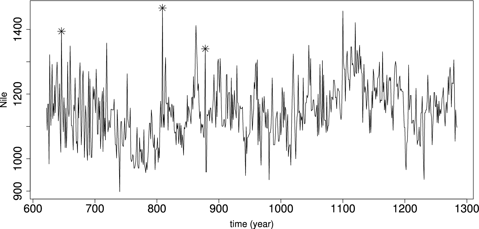
The question has been raised as to whether the Nile time series contains outliers; see for example Beran (1992), Robinson (1995), Chareka et al. (2006) and Fajardo et al. (2009). The test procedure developed by Chareka et al. (2006), suggests the presence of outliers at 646 AD (pp-value 0.0308) and at 809 (pp-value 0.0007). Another possible outlier is at 878 AD. A plot of the time series where the observations which have been judged to be outliers are marked, is shown in the left part of Figure 7, and the right part of this figure displays the histogram of the data. Although the theory developed in this paper is related to Gaussian processes, we believe that the small asymmetry of the data does not compromise the use of this series as an illustration of our robust methodology. A way to avoid this asymmetry is to consider the logarithm of the data. However, this does not make a significant difference in the estimates.
Refer to caption Refer to caption
Figure 7. Left: The Nile River data plot. Right: Histogram of the Nile River data.

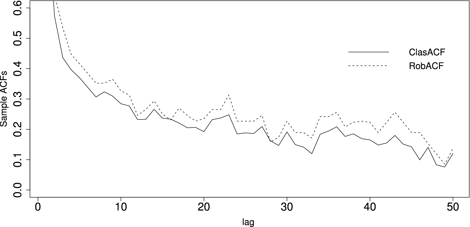
The left part of Figure 8 displays plots of the classical and robust sample autocorrelation functions of the original data. The autocorrelation values from the former are smaller than those of the latter one. However, the difference between the autocorrelations may be not large enough to suggest the presence of outliers. Thus, to better understand the influence of outliers on the sample autocorrelation functions in practical situations a new dataset with artificial outliers was generated. We replaced the presumed outliers detected by Chareka et al. (2006) by the mean plus 5 or 10 standard deviations. The sample autocorrelations (robust and classical ones) were again calculated, see the right part of Figure 8. As expected, the values of the robust autocorrelations remained stable. However, the classical autocorrelations were significantly affected by the increase of the size of the observation. This is in accordance with the results presented in the simulation section.
Refer to caption Refer to caption
Figure 8. Left: Classical (plain line) and robust (dotted line) sample autocorrelation functions of the Nile River data. Right: Classical (plain line) and robust (dotted line) sample autocorrelation functions of the Nile River data and classical sample autocorrelation functions of the Nile River data with artificial outliers at the times detected by Chareka et al. (2006) (original data plus 5 standard deviations with “ □\Box ” and original data plus 10 standard deviations with “ ▽\triangledown ”).

5. Asymptotic behavior of UU-processes

Consider the UU-process {UnG​(r),r∈I}\{U^{G}_{n}(r),r\in I\} satisfying

UnG(r)=1n⁡(n−1)∑1≤i≠j≤n𝟙{G(Xi,Xj)≤r},r∈IU^{G}_{n}(r)=\frac{1}{n(n-1)}\sum_{1\leq i\neq j\leq n}\mathbbm{1}_{\{G(X_{i},X_{j})\leq r\}}\;,r\in I (41)

based on the class of kernels

kG(x,y,r)=𝟙{G(x,y)≤r}.k_{G}(x,y,r)=\mathbbm{1}_{\{G(x,y)\leq r\}}\;. (42)

where II is an interval included in ℝ\mathbb{R}, GG is a symmetric function i.e. G⁡(x,y)=G⁡(y,x)G(x,y)=G(y,x) for all x,yx,y in ℝ\mathbb{R}, and the process (Xi)i≥1(X_{i})_{i\geq 1} satisfies Assumption (A(A2)) with γ⁡(0)=1\gamma(0)=1.

The asymptotic properties of these UU-processes have been studied in Lévy-Leduc et al. (2009). They are based on the computation of the Hermite rank of the class of functions {𝟙{G(⋅,⋅)≤r}−UG(r),r∈I}\{\mathbbm{1}_{\{G(\cdot,\cdot)\leq r\}}-U^{G}(r),r\in I\} where

UG(r)=∫ℝ2𝟙{G(x,y)≤r}ϕ(x)ϕ(y)dxdy,for allr∈I.U^{G}(r)=\int_{\mathbb{R}^{2}}\mathbbm{1}_{\{G(x,y)\leq r\}}\phi(x)\phi(y)\mathrm{d}x\mathrm{d}y\;,\;\text{for all}\;r\in I\;. (43)

The Hermite rank of the class of functions {𝟙{G(⋅,⋅)≤r}−U(r),r∈I}\{\mathbbm{1}_{\{G(\cdot,\cdot)\leq r\}}-U(r),r\in I\} is obtained by expanding the function 𝟙{G(⋅,⋅)≤r}\mathbbm{1}_{\{G(\cdot,\cdot)\leq r\}} in the basis of Hermite polynomials with leading coefficient equal to 1:

𝟙{G(x,y)≤r}=∑p,q≥0αp,q​(r)p!​q!Hp(x)Hq(y), for all x,y in ℝ,\mathbbm{1}_{\{G(x,y)\leq r\}}=\sum_{p,q\geq 0}\frac{\alpha_{p,q}(r)}{p!q!}H_{p}(x)H_{q}(y)\;,\textrm{ for all }x,y\textrm{ in }\mathbb{R}\;, (44)

where αp,q(r)=𝔼[𝟙{G(X,Y)≤r}Hp(X)Hq(Y)]\alpha_{p,q}(r)=\mathbb{E}\left[\mathbbm{1}_{\{G(X,Y)\leq r\}}H_{p}(X)H_{q}(Y)\right], XX and YY being independent standard Gaussian random variables. The first few Hermite polynomials are H0​(x)=1H_{0}(x)=1, H1​(x)=xH_{1}(x)=x, H2​(x)=x2−1H_{2}(x)=x^{2}-1, H3​(x)=x3−3​xH_{3}(x)=x^{3}-3x. Note that α0,0​(r)\alpha_{0,0}(r) is equal to UG​(r)U^{G}(r) for all rr, where UG​(r)U^{G}(r) is defined in (43). The previous expansion can also be rewritten as

𝟙{G(x,y)≤r}−UG(r)=∑p+q≥mp,q≥0αp,q​(r)p!​q!Hp(x)Hq(y),\mathbbm{1}_{\{G(x,y)\leq r\}}-U^{G}(r)=\sum_{\stackrel{{\scriptstyle p,q\geq 0}}{{p+q\geq m}}}\frac{\alpha_{p,q}(r)}{p!q!}H_{p}(x)H_{q}(y)\;, (45)

where m=m⁡(r)m=m(r) is called the Hermite rank of the function 𝟙{G(⋅,⋅)≤r}−UG(r)\mathbbm{1}_{\{G(\cdot,\cdot)\leq r\}}-U^{G}(r) when rr is fixed.

We state the results for family of kernels having Hermite rank equal to m=2m=2 (this is all we need here) and refer to Lévy-Leduc et al. (2009) for other cases.

Proposition 10.

Let II be a compact interval of ℝ\mathbb{R}, let kG​(⋅,⋅,r)k_{G}(\cdot,\cdot,r) be defined in (42), and let

kG,1​(x,r)=𝔼⁡[kG​(x,Y,r)],x∈ℝ,r∈I,\displaystyle k_{G,1}(x,r)=\mathbb{E}\left[k_{G}(x,Y,r)\right]\;,\;x\in\mathbb{R}\;,\;r\in I\;, (46)

where YY is a standard Gaussian variable. Suppose that the Hermite rank of the class of functions {kG​(⋅,⋅,r)−UG​(r),r∈I}\{k_{G}(\cdot,\cdot,r)-U^{G}(r)\;,r\in I\} is m=2m=2 and that Assumption (A(A2)) is satisfied with γ⁡(0)=1\gamma(0)=1 and 1/2<D<11/2<D<1. Assume that kGk_{G} satisfies the following three conditions:

  1. (i)

    There exists a positive constant CC such that for all ss, tt in II, uu, vv in ℝ\mathbb{R},

    𝔼⁡[|kG​(X+u,Y+v,s)−kG​(X+u,Y+v,t)|]≤C​|t−s|,\mathbb{E}\left[|k_{G}(X+u,Y+v,s)-k_{G}(X+u,Y+v,t)|\right]\leq\;C|t-s|\;, (47)

    where (X,Y)(X,Y) is a standard Gaussian random vector.

  2. (ii)

    There exists a positive constant CC such that for all ℓ≥1\ell\geq 1 and s,ts,t in II, uu, vv in ℝ\mathbb{R},

    𝔼⁡[|kG​(X1+u,X1+ℓ+v,t)−kG​(X1,X1+ℓ,t)|]≤C​|u−v|.\mathbb{E}\left[|k_{G}(X_{1}+u,X_{1+\ell}+v,t)-k_{G}(X_{1},X_{1+\ell},t)|\right]\leq C|u-v|\;. (48)
    𝔼⁡[|kG​(X1,X1+ℓ,s)−kG​(X1,X1+ℓ,t)|]≤C​|t−s|,\mathbb{E}\left[|k_{G}(X_{1},X_{1+\ell},s)-k_{G}(X_{1},X_{1+\ell},t)|\right]\leq C|t-s|\;, (49)
  3. (iii)

    There exists a positive constant CC such that for all tt in II, and xx, uu, vv in ℝ\mathbb{R},

    |kG,1​(x+u,t)−kG,1​(x+v,t)|≤C​|u−v|,\displaystyle|k_{G,1}(x+u,t)-k_{G,1}(x+v,t)|\leq C|u-v|\;, (50)
    |kG,1​(x,s)−kG,1​(x,t)|≤C​|t−s|.\displaystyle|k_{G,1}(x,s)-k_{G,1}(x,t)|\leq C|t-s|\;. (51)

Then the UU-process {n​(UnG​(r)−UG​(r)),r∈I}\{\sqrt{n}(U^{G}_{n}(r)-U^{G}(r)),r\in I\} defined in (41) and (43) converges weakly in the space of cadlag functions on II, 𝒟⁡(I)\mathcal{D}(I), equipped with the topology of uniform convergence to the zero mean Gaussian process {WG​(r),r∈I}\{W_{G}(r),r\in I\} with covariance structure given by

𝔼⁡[WG​(s)​WG​(t)]=4​Cov​(kG,1​(X1,s),kG,1​(X1,t))+4∑ℓ≥1Cov(kG,1(X1,s),kG,1(Xℓ+1,t))+Cov(kG,1(X1,t),kG,1(Xℓ+1,s)).\mathbb{E}[W_{G}(s)W_{G}(t)]=4\;\mathrm{Cov}(k_{G,1}(X_{1},s),k_{G,1}(X_{1},t))\\ +4\sum_{\ell\geq 1}\ \mathrm{Cov}(k_{G,1}(X_{1},s),k_{G,1}(X_{\ell+1},t))+\mathrm{Cov}(k_{G,1}(X_{1},t),k_{G,1}(X_{\ell+1},s))\;. (52)

Moreover, for a fixed rr in II, as nn tends to infinity,

n​(UnG​(r)−UG​(r))=2n​∑i=1n[kG,1​(Xi,r)−UG​(r)]+oP​(1).\sqrt{n}(U^{G}_{n}(r)-U^{G}(r))=\frac{2}{\sqrt{n}}\sum_{i=1}^{n}\left[k_{G,1}(X_{i},r)-U^{G}(r)\right]+o_{P}(1)\;. (53)

We now consider the case where D<1/2D<1/2. In this case, the normalization depends, as expected, on DD and the slowly varying function LL and the limiting distribution is no longer a Gaussian process. Let (Z1,D​(t))t∈ℝ+(Z_{1,D}(t))_{t\in\mathbb{R}_{+}} denote the standard fractional Brownian motion (fBm) and (Z2,D​(t))t∈ℝ+(Z_{2,D}(t))_{t\in\mathbb{R}_{+}} the Rosenblatt process. They are defined through multiple Wiener-Itô integrals and given by

Z1,D(t)=∫ℝ[∫0t(u−x)+−(D+1)/2du]dB(x),0<D<1,Z_{1,D}(t)=\int_{\mathbb{R}}\left[\int_{0}^{t}(u-x)_{+}^{-(D+1)/2}\mathrm{d}u\right]\mathrm{d}B(x),\quad 0<D<1\;, (54)

and

Z2,D(t)=∫ℝ2′[∫0t(u−x)+−(D+1)/2(u−y)+−(D+1)/2du]dB(x)dB(y), 0<D<1/2,Z_{2,D}(t)=\int^{\prime}_{\mathbb{R}^{2}}\left[\int_{0}^{t}(u-x)_{+}^{-(D+1)/2}(u-y)_{+}^{-(D+1)/2}du\right]\mathrm{d}B(x)\mathrm{d}B(y),\;0<D<1/2\;, (55)

where BB is the standard Brownian motion, see Fox and Taqqu (1987). The symbol ∫′\int^{\prime} means that the domain of integration excludes the diagonal. Introduce also the Beta function

B​(α,β)=∫0∞yα−1​(1+y)−α−β​𝑑y=Γ⁡(α)​Γ​(β)Γ⁡(α+β),α>0,β>0.\textrm{B}(\alpha,\beta)=\int_{0}^{\infty}y^{\alpha-1}(1+y)^{-\alpha-\beta}\mathrm{d}y=\frac{\Gamma(\alpha)\Gamma(\beta)}{\Gamma(\alpha+\beta)}\;,\quad\alpha>0,\;\beta>0\;. (56)
Proposition 11.

Let II be a compact interval of ℝ\mathbb{R} Suppose that the Hermite rank of the class of functions {kG​(⋅,⋅,r)−UG​(r),r∈I}\{k_{G}(\cdot,\cdot,r)-U^{G}(r)\;,r\in I\} is m=2m=2 and that Assumption (A(A2)) is satisfied with γ⁡(0)=1\gamma(0)=1 and D<1/2D<1/2. Assume the following:

  1. (i)

    There exists a positive constant C such that, for all ℓ≥1\ell\geq 1 and for all s,ts,t in II,

    𝔼⁡[|kG​(X1,X1+ℓ,s)−kG​(X1,X1+ℓ,t)|]≤C​|t−s|.\mathbb{E}[|k_{G}(X_{1},X_{1+\ell},s)-k_{G}(X_{1},X_{1+\ell},t)|]\leq C|t-s|\;. (57)
  2. (ii)

    UGU^{G} is a Lipschitz function

  3. (iii)

    The function Λ~\widetilde{\Lambda} defined, for all ss in II, by

    Λ~​(s)=𝔼⁡[kG​(X,Y,s)​(|X|+|X​Y|+|X2−1|)],\widetilde{\Lambda}(s)=\mathbb{E}[k_{G}(X,Y,s)(|X|+|XY|+|X^{2}-1|)]\;, (58)

    where XX and YY are independent standard Gaussian random variables, is also a Lipschitz function.

Then, the UU-process {UnG​(r)−UG​(r),r∈I}\{U_{n}^{G}(r)-U^{G}(r),r\in I\} defined in (41) and (43) has the following asymptotic properties:

{nD​L−1​(n)​(UnG​(r)−UG​(r));r∈I}\left\{n^{D}L^{-1}(n)\left(U_{n}^{G}(r)-U^{G}(r)\right);r\in I\right\}

converges weakly in the space of cadlag functions 𝒟⁡(I)\mathcal{D}(I), equipped with the topology of uniform convergence, to

{β​(D)−1​[α1,1​(r)​Z1,D​(1)2+α2,0​(r)​Z2,D​(1)];r∈I},\{\beta(D)^{-1}\left[\alpha_{1,1}(r)Z_{1,D}(1)^{2}+\alpha_{2,0}(r)Z_{2,D}(1)\right];r\in I\}\;,

where the fractional Brownian motion Z1,D​(⋅)Z_{1,D}(\cdot) and the Rosenblatt process Z2,D​(⋅)Z_{2,D}(\cdot) are defined in (54) and (55) respectively and where β⁡(D)=B​((1−D)/2,D)\beta(D)=\emph{\textrm{B}}((1-D)/2,D), B denoting the Beta function, defined in (56).

Propositions 10 and 11 will be applied to the UU-process Un​(r)U_{n}(r) in (36) with

U(r)=∫ℝ2𝟙{∥x−y|≤r}dF(x)dF(y)=T1(F)[r],U(r)=\int_{\mathbb{R}^{2}}\mathbbm{1}_{\{\|x-y|\leq r\}}\mathrm{d}F(x)\mathrm{d}F(y)=T_{1}(F)[r]\;, (59)

with T1T_{1} given in (13). By Lemma 14, the Hermite rank of the class of functions {𝟙|x−y|≤r−U⁡(r),x,y∈ℝ,r∈I}\{\mathbbm{1}_{|x-y|\leq r}-U(r),x,y\in\mathbb{R},r\in I\} is equal to 2 where I=[r0−η,r0+η]I=[r_{0}-\eta,r_{0}+\eta] for some positive η\eta defined in Lemma 14 and where r0=1/c⁡(Φ)r_{0}=1/c(\Phi) (see (10)) is such that

T1​(Φ)​[r0]=T1​(Φ)​[1/c⁡(Φ)]=1/4.T_{1}(\Phi)[r_{0}]=T_{1}(\Phi)[1/c(\Phi)]=1/4\;. (60)

6. Proofs

Proof of Lemma 1.

Denote by FF the c.d.f. Φμ,σ\Phi_{\mu,\sigma} of X1X_{1}. Since an​(Fn−F)a_{n}(F_{n}-F) converges in distribution in the space of cadlag functions equipped with the topology of uniform convergence, the asymptotic expansion (18) can be deduced from the functional Delta method stated e.g. in Theorem 20.8 of van der Vaart (1998). To show this, we have to prove that T0=T1∘T2T_{0}=T_{1}\circ T_{2} is Hadamard differentiable, where T1T_{1} and T2T_{2} are defined in (13) and (14) respectively and that the corresponding Hadamard differential is defined and continuous on the whole space of cadlag functions. For a definition of Hadamard differentiability, we refer to (van der Vaart, 1998, Chapter 20).

We prove first that the Hadamard differentiability of the functional T1T_{1} defined in (13). Let (gt)(g_{t}) be a sequence of cadlag functions with bounded variations such that ‖gt−g‖∞→0\left\|g_{t}-g\right\|_{\infty}\to 0, as t→0t\to 0, where gg is a cadlag function. For any non negative rr, we consider

t−1​{T1​(F+t​gt)​[r]−T1​(F)​[r]}=2∫ℝ∫ℝ𝟙{|x−y|≤r}dF(x)dgt(y)+t∫ℝ∫ℝ𝟙{|x−y|≤r}dgt(x)dgt(y).t^{-1}\left\{T_{1}(F+tg_{t})[r]-T_{1}(F)[r]\right\}\\ =2\int_{\mathbb{R}}\int_{\mathbb{R}}\mathbbm{1}_{\{|x-y|\leq r\}}\mathrm{d}F(x)\mathrm{d}g_{t}(y)+t\int_{\mathbb{R}}\int_{\mathbb{R}}\mathbbm{1}_{\{|x-y|\leq r\}}\mathrm{d}g_{t}(x)\mathrm{d}g_{t}(y)\;.

Since

|∫ℝ∫ℝ𝟙{|x−y|≤r}dF(x)dgt(y)−∫ℝ∫ℝ𝟙{|x−y|≤r}dF(x)dg(y)|=|∫ℝ(gt​(x+r)−g⁡(x+r))​dF​(x)−∫ℝ(gt​(x−r)−g⁡(x−r))​dF​(x)|≤2​‖gt−g‖∞→0,\left|\int_{\mathbb{R}}\int_{\mathbb{R}}\mathbbm{1}_{\{|x-y|\leq r\}}\mathrm{d}F(x)\mathrm{d}g_{t}(y)-\int_{\mathbb{R}}\int_{\mathbb{R}}\mathbbm{1}_{\{|x-y|\leq r\}}\mathrm{d}F(x)\mathrm{d}g(y)\right|\\ =\left|\int_{\mathbb{R}}\left(g_{t}(x+r)-g(x+r)\right)\mathrm{d}F(x)-\int_{\mathbb{R}}\left(g_{t}(x-r)-g(x-r)\right)\mathrm{d}F(x)\right|\leq 2\left\|g_{t}-g\right\|_{\infty}\to 0\;,

as tt tends to zero, the Hadamard differential of T1T_{1} at gg is given by:

(DT1(F).g)(r)=2∫ℝ∫ℝ𝟙{|x−y|≤r}dF(x)dg(y)=2∫ℝ{g(x+r)−g(x−r)}dF(x).(DT_{1}(F).g)(r)=2\int_{\mathbb{R}}\int_{\mathbb{R}}\mathbbm{1}_{\{|x-y|\leq r\}}\ \mathrm{d}F(x)\mathrm{d}g(y)=2\int_{\mathbb{R}}\{g(x+r)-g(x-r)\}\mathrm{d}F(x)\;.

By Lemma 21.3 in van der Vaart (1998), T2T_{2} is Hadamard differentiable. Finally, using the Chain rule (Theorem 20.9 in van der Vaart (1998)), we obtain the Hadamard differentiability of T0T_{0} with the following Hadamard differential:

D​T0​(F).g=−(DT1(F).g)(T0(F))(T1​(F))′​[T0​(F)]=−2​∫ℝ{g⁡(x+T0​(F))−g⁡(x−T0​(F))}​𝑑F​(x)(T1​(F))′​[T0​(F)].DT_{0}(F).g=-\frac{(DT_{1}(F).g)(T_{0}(F))}{(T_{1}(F))^{\prime}[T_{0}(F)]}=-\frac{2\int_{\mathbb{R}}\{g(x+T_{0}(F))-g(x-T_{0}(F))\}\mathrm{d}F(x)}{(T_{1}(F))^{\prime}[T_{0}(F)]}\;. (61)

In view of the last expression, D​T0​(F)DT_{0}(F) is a continuous function of gg and is defined on the whole space of cadlag functions. Thus, by Theorem 20.8 of van der Vaart (1998), we obtain:

an(Qn(X1:n,Φ)−Q(F))=c(Φ)DT0(F).{an(Fn−F)}+oP(1),a_{n}(\mathrm{Q}_{n}\left(X_{1:n},\Phi\right)-Q(F))=c(\Phi)\;DT_{0}(F).\{a_{n}(F_{n}-F)\}+o_{P}(1)\;, (62)

where c⁡(Φ)c(\Phi) is the constant defined in (10). By (13), T1​(F)​[r]=∫ℝ[F⁡(x+r)−F⁡(x−r)]​𝑑F​(x)T_{1}(F)[r]=\int_{\mathbb{R}}[F(x+r)-F(x-r)]\mathrm{d}F(x) and since F(⋅)=Φμ,σ(⋅)=Φ((⋅−μ)/σ)F(\cdot)=\Phi_{\mu,\sigma}(\cdot)=\Phi((\cdot-\mu)/\sigma), we get

(T1​(F))′​[r]=2σ​∫ℝΦ⁡(y+rσ)​Φ​(y)​𝑑y.(T_{1}(F))^{\prime}[r]=\frac{2}{\sigma}\int_{\mathbb{R}}\Phi\left(y+\frac{r}{\sigma}\right)\Phi(y)\mathrm{d}y\;.

Since σ=Q⁡(Φμ,σ)=c⁡(Φ)​T0​(F)\sigma=Q(\Phi_{\mu,\sigma})=c(\Phi)T_{0}(F) by (5), we get

(T1​(F))′​[T0​(F)]=2​σ−1​∫ϕ⁡(y)​ϕ​(y+1/c⁡(Φ))​𝑑y.(T_{1}(F))^{\prime}[T_{0}(F)]=2\sigma^{-1}\int\phi(y)\phi(y+1/c(\Phi))\mathrm{d}y\;. (63)

Applying (61) with T0​(F)=σ/c⁡(Φ)T_{0}(F)=\sigma/c(\Phi), using (63), and setting g=an​(Fn−F)g=a_{n}(F_{n}-F), we get

D​T0​(F).{an​(Fn−F)}=An−Bn,DT_{0}(F).\{a_{n}(F_{n}-F)\}=A_{n}-B_{n}\;, (64)

where

An=an​((T1​(F))′​[T0​(F)])−1​∫ℝ{F⁡(x+σc⁡(Φ))−F⁡(x−σc⁡(Φ))}​𝑑F​(x)A_{n}=a_{n}\left((T_{1}(F))^{\prime}[T_{0}(F)]\right)^{-1}\int_{\mathbb{R}}\left\{F\left(x+\frac{\sigma}{c(\Phi)}\right)-F\left(x-\frac{\sigma}{c(\Phi)}\right)\right\}\mathrm{d}F(x) (65)

and BnB_{n} has the same expression with FF replaced by FnF_{n}. The integral in AnA_{n} equals

∫ℝ∫ℝ𝟙{|y−x|≤σ/c(Φ)}dF(x)dF(y)=T1(F)[T0(F)]=1/4,\int_{\mathbb{R}}\int_{\mathbb{R}}\mathbbm{1}_{\{|y-x|\leq\sigma/c(\Phi)\}}\mathrm{d}F(x)\mathrm{d}F(y)=T_{1}(F)[T_{0}(F)]=1/4\;, (66)

by definition (see (5)). The corresponding integral in BnB_{n} equals

1n​∑i=1n{F⁡(Xi+σc⁡(Φ))−F⁡(Xi−σc⁡(Φ))}=1n​∑i=1n{Φ⁡(Xi−μσ+1c⁡(Φ))−Φ⁡(Xi−μσ−1c⁡(Φ))}.\frac{1}{n}\sum_{i=1}^{n}\left\{F\left(X_{i}+\frac{\sigma}{c(\Phi)}\right)-F\left(X_{i}-\frac{\sigma}{c(\Phi)}\right)\right\}\\ =\frac{1}{n}\sum_{i=1}^{n}\left\{\Phi\left(\frac{X_{i}-\mu}{\sigma}+\frac{1}{c(\Phi)}\right)-\Phi\left(\frac{X_{i}-\mu}{\sigma}-\frac{1}{c(\Phi)}\right)\right\}\;.

The result follows from (62), (61), (64), (63) and the above expressions for AnA_{n} and BnB_{n}. ∎

Proof of Theorem 2.

Assumption (A(A1)) and the Theorem of Csörgő and Mielniczuk (1996) implies that n​(Fn−Φ0,σ)\sqrt{n}(F_{n}-\Phi_{0,\sigma}) converges in distribution to a Gaussian process in the space of cadlag functions equipped with the topology of uniform convergence. Thus, the asymptotic expansion of an(Qn(X1:n,Φ)−σ)a_{n}(\mathrm{Q}_{n}\left(X_{1:n},\Phi\right)-\sigma) obtained in (18) is valid with an=na_{n}=\sqrt{n}. We thus have to prove a CLT for n−1/2∑i=1nIF(Xi/σ,Q,Φ)n^{-1/2}\sum_{i=1}^{n}\mathrm{IF}(X_{i}/\sigma,Q,\Phi). Using Lemma 12 below, we note that the Hermite rank of IF⁡(⋅,Q,Φ)\mathrm{IF}(\cdot,Q,\Phi) is equal to 2 and the conclusion follows by applying (Breuer and Major, 1983, Theorem 1). ∎

Proof of Proposition 3.

Note that σ^n,X2=γ⁡(0)​σ^n,Y2\widehat{\sigma}^{2}_{n,X}=\gamma(0)\widehat{\sigma}^{2}_{n,Y}, where (Yi)i≥1(Y_{i})_{i\geq 1} satisfies (A(A1)) with γ⁡(0)=1\gamma(0)=1. Observe that σ^n,Y2−1\widehat{\sigma}^{2}_{n,Y}-1 is a UU-statistic with kernel k⁡(x,y)=(x−y)2/2−1k(x,y)=(x-y)^{2}/2-1. The Hoeffding decomposition of this kernel is given by k⁡(x,y)=(x2−1)/2+(y2−1)/2−x​yk(x,y)=(x^{2}-1)/2+(y^{2}-1)/2-xy. From this, we obtain the corresponding Hoeffding decomposition of σ^n,Y2−1\widehat{\sigma}^{2}_{n,Y}-1 as

σ^n,Y2−1=1n​∑i=1nH2​(Yi)−1n⁡(n−1)​∑1≤i≠j≤nYi​Yj.\widehat{\sigma}^{2}_{n,Y}-1=\frac{1}{n}\sum_{i=1}^{n}H_{2}(Y_{i})-\frac{1}{n(n-1)}\sum_{1\leq i\neq j\leq n}Y_{i}Y_{j}\;. (67)

Under Assumption (A(A1)), the first term of this decomposition is the leading one. Then, using (Breuer and Major, 1983, Theorem 1), we get that n​(σ^n,X2−σ2)\sqrt{n}(\widehat{\sigma}^{2}_{n,X}-\sigma^{2}) converges to a zero-mean Gaussian random variable having a variance equal to 2​(γ​(0)2+2​∑k≥1γ​(k)2)2(\gamma(0)^{2}+2\sum_{k\geq 1}\gamma(k)^{2}). Using the Delta method to go from σ^n,X2\widehat{\sigma}^{2}_{n,X} to σ^n,X\widehat{\sigma}_{n,X}, setting f⁡(x)=xf(x)=\sqrt{x}, so that f′​(σ2)=1/(2​σ2)=1/(2​σ)f^{\prime}(\sigma^{2})=1/(2\sqrt{\sigma^{2}})=1/(2\sigma), we get that the asymptotic variance of n​(σ^n,X−σ)\sqrt{n}\left(\widehat{\sigma}_{n,X}-\sigma\right) is thus equal to (28).

By Lemma 12, the Hermite rank of IF(.,Q,Φ)\mathrm{IF}(.,Q,\Phi) is equal to 2, hence using (Arcones, 1994, Lemma 1), σ~2\widetilde{\sigma}^{2} defined in (26) satisfies

σ~2≤γ​(0)−1​𝔼​[IF​(X1/σ,Q,Φ)2]​{γ​(0)2+2​∑k≥1γ​(k)2}.\widetilde{\sigma}^{2}\leq\gamma(0)^{-1}\mathbb{E}[\mathrm{IF}(X_{1}/\sigma,Q,\Phi)^{2}]\{\gamma(0)^{2}+2\sum_{k\geq 1}\gamma(k)^{2}\}\;.

Finally, in this case, using that 𝔼⁡[IF​(X1/σ,Q,Φ)2]≈0.6077\mathbb{E}[\mathrm{IF}(X_{1}/\sigma,Q,\Phi)^{2}]\approx 0.6077 (Rousseeuw and Croux, 1993, p. 1278), the relative asymptotic efficiency σ~c​l2/σ~2\widetilde{\sigma}^{2}_{cl}/\widetilde{\sigma}^{2} of Qn(X1:n,Φ)\mathrm{Q}_{n}\left(X_{1:n},\Phi\right) compared to σ^n,X\widehat{\sigma}_{n,X} is larger than 82.27%82.27\% since

(2​γ​(0))−1​(γ​(0)2+2​∑k≥1γ​(k)2)γ​(0)−1​𝔼​[IF​(X1/σ,Q,Φ)2]​{γ​(0)2+2​∑k≥1γ​(k)2}≈0.5/0.6077≈82.27%.\frac{(2\gamma(0))^{-1}(\gamma(0)^{2}+2\sum_{k\geq 1}\gamma(k)^{2})}{\gamma(0)^{-1}\mathbb{E}[\mathrm{IF}(X_{1}/\sigma,Q,\Phi)^{2}]\{\gamma(0)^{2}+2\sum_{k\geq 1}\gamma(k)^{2}\}}\approx 0.5/0.6077\approx 82.27\%\;.

∎

Proof of Theorem 4.

Let Φσ,+\Phi_{\sigma,+} and Φσ,−\Phi_{\sigma,-} denote the c.d.f of (Xi+Xi+h)i≥1(X_{i}+X_{i+h})_{i\geq 1} and (Xi−Xi+h)i≥1(X_{i}-X_{i+h})_{i\geq 1}, respectively. Let also denote by F+,n−hF_{+,n-h} and F−,n−hF_{-,n-h} the empirical c.d.f of (Xi+Xi+h)1≤i≤n−h(X_{i}+X_{i+h})_{1\leq i\leq n-h} and (Xi−Xi+h)1≤i≤n−h(X_{i}-X_{i+h})_{1\leq i\leq n-h}, respectively. Since (Xi)i≥1(X_{i})_{i\geq 1} satisfy Assumption (A(A1)), it is the same for (Xi+Xi+h)i≥1(X_{i}+X_{i+h})_{i\geq 1} and (Xi−Xi+h)i≥1(X_{i}-X_{i+h})_{i\geq 1} with scales equal to Q⁡(Φσ,+)Q(\Phi_{\sigma,+}) and Q⁡(Φσ,−)Q(\Phi_{\sigma,-}), respectively. Thus, using the Theorem of Csörgő and Mielniczuk (1996), we obtain that n−h​(F+,n−h−Φσ,+)\sqrt{n-h}(F_{+,n-h}-\Phi_{\sigma,+}) converges in distribution to a Gaussian process in the space of cadlag functions equipped with the topology of uniform convergence and that the same holds for n−h​(F−,n−h−Φσ,−)\sqrt{n-h}(F_{-,n-h}-\Phi_{\sigma,-}). As a consequence, the expansion (18) is valid for Qn−h(X1:n−h+Xh+1:n,Φ)\mathrm{Q}_{n-h}\left(X_{1:n-h}+X_{h+1:n},\Phi\right) and Qn−h(X1:n−h−Xh+1:n,Φ)\mathrm{Q}_{n-h}\left(X_{1:n-h}-X_{h+1:n},\Phi\right) with an−h=n−ha_{n-h}=\sqrt{n-h}, that is

n−h[Qn−h(X1:n−h±Xh+1:n,Φ)−Q(Φσ,±)]=1n−h∑i=1n−hIF(Xi±Xi+h,Q,Φσ,±)+oP(1).\sqrt{n-h}\left[\mathrm{Q}_{n-h}\left(X_{1:n-h}\pm X_{h+1:n},\Phi\right)-Q(\Phi_{\sigma,\pm})\right]=\frac{1}{\sqrt{n-h}}\sum_{i=1}^{n-h}\mathrm{IF}(X_{i}\pm X_{i+h},Q,\Phi_{\sigma,\pm})+o_{P}(1)\;.

Then, applying the Delta method (van der Vaart, 1998, Theorem 3.1) with the transformation b⁡(x)=x2b(x)=x^{2}, b′​(x)=2​xb^{\prime}(x)=2x, we get

n−h[Qn−h(X1:n−h±Xh+1:n,Φ)2−Q2(Φσ,±)]=2​Q​(Φσ,±)n−h​∑i=1n−hIF⁡(Xi±Xi+h,Q,Φσ,±)+oP​(1).\sqrt{n-h}\left[\mathrm{Q}_{n-h}\left(X_{1:n-h}\pm X_{h+1:n},\Phi\right)^{2}-Q^{2}(\Phi_{\sigma,\pm})\right]\\ =\frac{2Q(\Phi_{\sigma,\pm})}{\sqrt{n-h}}\sum_{i=1}^{n-h}\mathrm{IF}(X_{i}\pm X_{i+h},Q,\Phi_{\sigma,\pm})+o_{P}(1)\;.

Hence γ^Q(h,X1:n,Φ)\widehat{\gamma}_{Q}(h,X_{1:n},\Phi) in (29) satisfies the following asymptotic expansion:

n−h(γ^Q(h,X1:n,Φ)−{Q2(Φσ,+)−Q2(Φσ,−)}/4)=1n−h∑i=1n−hψ(Xi,Xi+h)+oP(1),\sqrt{n-h}\left(\widehat{\gamma}_{Q}(h,X_{1:n},\Phi)-\left\{Q^{2}(\Phi_{\sigma,+})-Q^{2}(\Phi_{\sigma,-})\right\}/4\right)=\frac{1}{\sqrt{n-h}}\sum_{i=1}^{n-h}\psi(X_{i},X_{i+h})+o_{P}(1)\;, (68)

where for all xx and yy,

ψ⁡(x,y)=12​{Q⁡(Φσ,+)​IF​(x+y,Q,Φσ,+)−Q⁡(Φσ,−)​IF​(x−y,Q,Φσ,−)}.\psi(x,y)=\frac{1}{2}\left\{Q(\Phi_{\sigma,+})\;\mathrm{IF}\left(x+y,Q,\Phi_{\sigma,+}\right)-Q(\Phi_{\sigma,-})\;\mathrm{IF}\left(x-y,Q,\Phi_{\sigma,-}\right)\right\}\;.

Using the identity (19), ψ\psi has the expression given in (31). We have now to prove a CLT for (n−h)−1/2∑i=1n−hψ(Xi,Xi+h)(n-h)^{-1/2}\sum_{i=1}^{n-h}\psi(X_{i},X_{i+h}). Using Lemma 13, the definition of the Hermite rank given in (Arcones, 1994, p. 2245) and Assumption (A(A1)), we obtain that Condition (2.40) of Theorem 4 (Arcones, 1994, p. 2256) is satisfied with τ=2\tau=2. This concludes the proof of the theorem by observing that {Q2​(Φσ,+)−Q2​(Φσ,−)}/4=𝔼⁡[X1​X1+h]=γ⁡(h)\{Q^{2}(\Phi_{\sigma,+})-Q^{2}(\Phi_{\sigma,-})\}/4=\mathbb{E}[X_{1}X_{1+h}]=\gamma(h) (see 7). ∎

Proof of Theorem 6.

Since, by scale invariance, Qn(X1:n,Φ)−σ=σ(Qn(X1:n/σ,Φ)−1)\mathrm{Q}_{n}\left(X_{1:n},\Phi\right)-\sigma=\sigma(\mathrm{Q}_{n}\left(X_{1:n}/\sigma,\Phi\right)-1), we shall focus in the sequel on the case γ⁡(0)=1\gamma(0)=1. First, note that using Lemma 14 below the Hermite rank of the class of functions {𝟙{|⋅−⋅|≤r}−U(r),r∈[r0−η,r0+η]}\{\mathbbm{1}_{\{|\cdot-\cdot|\leq r\}}-U(r)\;,r\in[r_{0}-\eta,r_{0}+\eta]\} is m=2m=2, where UU is defined in (59) and r0r_{0} in (60).

(i) Suppose first D>1/2D>1/2. Let us verify that the assumptions of Proposition 10 hold. Conditions (47) and (48) are easily verified. Let us check Condition (49). Note that for all ℓ≥1\ell\geq 1, X1−X1+ℓ∼𝒩⁡(0,2​(1−γ⁡(ℓ)))X_{1}-X_{1+\ell}\sim\mathcal{N}(0,2(1-\gamma(\ell))), thus if t≤st\leq s, there exists a positive constant CC such that,

𝔼⁡[k⁡(X1,X1+ℓ,s)−k⁡(X1,X1+ℓ,t)]=ℙ⁡(t≤|X1−X1+ℓ|≤s)≤24​π​(1−γ⁡(ℓ))|t−s|≤C​|t−s|,\mathbb{E}[k(X_{1},X_{1+\ell},s)-k(X_{1},X_{1+\ell},t)]=\mathbb{P}(t\leq|X_{1}-X_{1+\ell}|\leq s)\leq\frac{2}{\sqrt{4\pi(1-\gamma(\ell))}}|t-s|\leq C|t-s|\;,

where k(x,y,r)=𝟙{|x−y|≤r}k(x,y,r)=\mathbbm{1}_{\{|x-y|\leq r\}}. Since γ⁡(ℓ)→0\gamma(\ell)\to 0 as ℓ→∞\ell\to\infty, we obtain (49).

Conditions (50) and (51) are satisfied since

k1(x,r)=𝔼[𝟙{|x−Y|≤r}]=Φ(x+r)−Φ(x−r).k_{1}(x,r)=\mathbb{E}[\mathbbm{1}_{\{|x-Y|\leq r\}}]=\Phi(x+r)-\Phi(x-r)\;. (69)

Now consider the process

{n​(T1​(Fn)​[r]−T1​(F)​[r]),r∈[r0−η,r0+η]},\{\sqrt{n}(T_{1}(F_{n})[r]-T_{1}(F)[r]),r\in[r_{0}-\eta,r_{0}+\eta]\}\;, (70)

where F=ΦF=\Phi and

T1(F)[r]=∫ℝ2𝟙{|y−x|≤r}dΦ(x)dΦ(y)=∫ℝ[Φ(x+r)−Φ(x−r)]dΦ(x).T_{1}(F)[r]=\int_{\mathbb{R}^{2}}\mathbbm{1}_{\{|y-x|\leq r\}}\mathrm{d}\Phi(x)\mathrm{d}\Phi(y)=\int_{\mathbb{R}}[\Phi(x+r)-\Phi(x-r)]\mathrm{d}\Phi(x)\;.

By Proposition 10, the process (70) converges weakly to a Gaussian process in the space of cadlag functions equipped with the topology of uniform convergence for some η>0\eta>0 when D>1/2D>1/2.

(ii) Suppose now D<1/2D<1/2. Let us check that the assumptions of Proposition 11 hold. Condition (57) holds since it is the same as Condition (49). Since k1k_{1} is a Lipschitz function, so is UU defined in (59). Let us now check Condition (58). If s≤ts\leq t

∫ℝ∫ℝ𝟙{s<x−y≤t}(|x|+|xy|+|x2−1|)ϕ(x)ϕ(y)dxdy=∫ℝ(∫x−tx−sϕ(y)dy)|x|ϕ(x)dx+∫ℝ(∫x−tx−s|y|ϕ(y)dy)|x|ϕ(x)dx+∫ℝ(∫x−tx−sϕ(y)dy)|x2−1|ϕ(x)dx.\int_{\mathbb{R}}\int_{\mathbb{R}}\mathbbm{1}_{\{s<x-y\leq t\}}(|x|+|xy|+|x^{2}-1|)\phi(x)\phi(y)\mathrm{d}x\mathrm{d}y=\int_{\mathbb{R}}\left(\int_{x-t}^{x-s}\phi(y)\mathrm{d}y\right)|x|\phi(x)\mathrm{d}x\\ +\int_{\mathbb{R}}\left(\int_{x-t}^{x-s}|y|\phi(y)\mathrm{d}y\right)|x|\phi(x)\mathrm{d}x+\int_{\mathbb{R}}\left(\int_{x-t}^{x-s}\phi(y)\mathrm{d}y\right)|x^{2}-1|\phi(x)\mathrm{d}x\;.

Since ϕ⁡(⋅)\phi(\cdot) and |.|ϕ(⋅)|.|\phi(\cdot) are bounded and that the moments of Gaussian random variables are all finite, we get (58). Then, applying Proposition 11 and Lemma 14 leads to the weak convergence of the process {β⁡(D)​nD/L⁡(n)​(T1​(Fn)​[r]−T1​(F)​[r]),r∈[r0−η,r0+η]}\{\beta(D)n^{D}/L(n)(T_{1}(F_{n})[r]-T_{1}(F)[r]),r\in[r_{0}-\eta,r_{0}+\eta]\} to {ϕ˙​(r/2)​(Z2,D​(1)−Z1,D​(1)2);r∈[r0−η,r0+η]}\{\dot{\phi}(r/\sqrt{2})(Z_{2,D}(1)-Z_{1,D}(1)^{2});r\in[r_{0}-\eta,r_{0}+\eta]\}.

We now want to use the functional Delta method as in the proof of Lemma 1 in both cases (i) and (ii).

By (van der Vaart, 1998, Lemma 21.3), T2T_{2} defined in (14) is Hadamard differentiable with the following Hadamard differential: DT2(T1(Φ))⋅g=−g(r0)/(T1(Φ))′[r0].DT_{2}(T_{1}(\Phi))\cdot g=-g(r_{0})/(T_{1}(\Phi))^{\prime}[r_{0}]\;. Thus D​T2​(T1​(Φ))DT_{2}(T_{1}(\Phi)) is a continuous function with respect to gg. By the functional Delta method, with T0=T2∘T1T_{0}=T_{2}\circ T_{1}, we obtain the following expansion:

an(Qn(X1:n,Φ)−Q(Φ))=c(Φ)an(T0(Fn)−T0(Φ))=−c(Φ)an(T1​(Fn)−T1​(Φ))​[r0](T1​(Φ))′​[r0]+oP(1),a_{n}(\mathrm{Q}_{n}\left(X_{1:n},\Phi\right)-Q(\Phi))=c(\Phi)\;a_{n}(T_{0}(F_{n})-T_{0}(\Phi))=-c(\Phi)\;a_{n}\frac{(T_{1}(F_{n})-T_{1}(\Phi))[r_{0}]}{(T_{1}(\Phi))^{\prime}[r_{0}]}+o_{P}(1)\;, (71)

where an=na_{n}=\sqrt{n} in the case (i)(i) and an=β⁡(D)​nD/L⁡(n)a_{n}=\beta(D)n^{D}/L(n) in the case (i​i)(ii). In case (i)(i),

−c⁡(Φ)​n​(T1​(Fn)−T1​(Φ))​[r0](T1​(Φ))′​[r0]⟶d𝒩⁡(0,σ12),-c(\Phi)\sqrt{n}\frac{(T_{1}(F_{n})-T_{1}(\Phi))[r_{0}]}{(T_{1}(\Phi))^{\prime}[r_{0}]}\stackrel{{\scriptstyle d}}{{\longrightarrow}}\mathcal{N}(0,\sigma^{2}_{1})\;,

where σ12\sigma^{2}_{1} is given by Equation (52) in Proposition 10:

σ12=4​Var[−c⁡(Φ)(T1​(Φ))′​[r0]​k1​(X1,r0)]+8∑k≥1Cov[−c⁡(Φ)(T1​(Φ))′​[r0]k1(X1,r0),−c⁡(Φ)(T1​(Φ))′​[r0]k1(Xk+1,r0)],\sigma^{2}_{1}=4\mathop{\rm Var}\nolimits\left[-\frac{c(\Phi)}{(T_{1}(\Phi))^{\prime}[r_{0}]}k_{1}(X_{1},r_{0})\right]\\ +8\sum_{k\geq 1}\mathrm{Cov}\left[-\frac{c(\Phi)}{(T_{1}(\Phi))^{\prime}[r_{0}]}k_{1}(X_{1},r_{0}),-\frac{c(\Phi)}{(T_{1}(\Phi))^{\prime}[r_{0}]}k_{1}(X_{k+1},r_{0})\right]\;, (72)

where k1k_{1} is defined in (69). Since

𝔼[k1(X1,r0)]=𝔼[Φ(X1+r0)−Φ(X1−r0)]=∫ℝ2𝟙{|y−x|≤r}dΦ(x)dΦ(y)=1/4\mathbb{E}[k_{1}(X_{1},r_{0})]=\mathbb{E}[\Phi(X_{1}+r_{0})-\Phi(X_{1}-r_{0})]=\int_{\mathbb{R}^{2}}\mathbbm{1}_{\{|y-x|\leq r\}}\mathrm{d}\Phi(x)\mathrm{d}\Phi(y)=1/4

by (60) and r0=1/c⁡(Φ)r_{0}=1/c(\Phi) by (9), we get using (63) that

−2​c​(Φ)​[k1​(X1,r0)−𝔼⁡(k1​(X1,r0))](T1​(Φ))′​[r0]=c⁡(Φ)​1/4+Φ⁡(X1−1/c⁡(Φ))−Φ⁡(X1+1/c⁡(Φ))2​∫ℝϕ⁡(y)​ϕ​(y+1/c⁡(Φ))​𝑑y=IF⁡(X1,Q,Φ),\frac{-2c(\Phi)\left[k_{1}(X_{1},r_{0})-\mathbb{E}(k_{1}(X_{1},r_{0}))\right]}{(T_{1}(\Phi))^{\prime}[r_{0}]}\\ =c(\Phi)\frac{1/4+\Phi(X_{1}-1/c(\Phi))-\Phi(X_{1}+1/c(\Phi))}{2\int_{\mathbb{R}}\phi(y)\phi(y+1/c(\Phi))\mathrm{d}y}=\mathrm{IF}(X_{1},Q,\Phi)\;, (73)

where IF⁡(⋅,Q,Φ)\mathrm{IF}(\cdot,Q,\Phi) is defined in (20). Using (72), (73) and (83) in Lemma 12, we get that

σ12=𝔼⁡[IF⁡(X1,Q,Φ)]+2​∑k≥1𝔼⁡[IF⁡(X1,Q,Φ)​IF​(Xk+1,Q,Φ)],\sigma^{2}_{1}=\mathbb{E}[\mathrm{IF}(X_{1},Q,\Phi)]+2\sum_{k\geq 1}\mathbb{E}[\mathrm{IF}(X_{1},Q,\Phi)\mathrm{IF}(X_{k+1},Q,\Phi)]\;,

which concludes the proof of (i)(i). In the case (i​i)(ii), in view of (71), it is sufficient to show that

−c⁡(Φ)​β​(D)​nDL⁡(n)​(T1​(Fn)−T1​(Φ))​[r0](T1​(Φ))′​[r0]⟶d12​(Z2,D​(1)−Z1,D​(1)2).-c(\Phi)\beta(D)\frac{n^{D}}{L(n)}\frac{(T_{1}(F_{n})-T_{1}(\Phi))[r_{0}]}{(T_{1}(\Phi))^{\prime}[r_{0}]}\stackrel{{\scriptstyle d}}{{\longrightarrow}}\frac{1}{2}(Z_{2,D}(1)-Z_{1,D}(1)^{2})\;. (74)

This result follows from the convergence in distribution of β⁡(D)​nD/L⁡(n)​(T1​(Fn)​[r0]−T1​(Φ)​[r0])\beta(D)n^{D}/L(n)(T_{1}(F_{n})[r_{0}]-T_{1}(\Phi)[r_{0}]) to ϕ˙​(r0/2)​(Z2,D​(1)−Z1,D​(1)2)\dot{\phi}(r_{0}/\sqrt{2})(Z_{2,D}(1)-Z_{1,D}(1)^{2}), (63) and the identity −c⁡(Φ)​ϕ˙​(r0/2)​(2​∫ℝϕ⁡(y)​ϕ​(y+r0)​𝑑y)−1=1/2.-c(\Phi)\;\dot{\phi}(r_{0}/\sqrt{2})(2\int_{\mathbb{R}}\phi(y)\phi(y+r_{0})\mathrm{d}y)^{-1}=1/2. This identity follows from ϕ˙(r0/2)=−(2π)−1exp(−r02/4)r0\dot{\phi}(r_{0}/\sqrt{2})=-(2\sqrt{\pi})^{-1}\exp(-r_{0}^{2}/4)r_{0} and r0=1/c⁡(Φ)r_{0}=1/c(\Phi). ∎

Proof of Proposition 7.

Using the same arguments as those used in the proof of Proposition 3, we get that σ^n,Y2−1\widehat{\sigma}^{2}_{n,Y}-1 satisfies the Hoeffding decomposition (67), where (Yi)i≥1(Y_{i})_{i\geq 1} satisfies (A(A2)) with γ⁡(0)=1\gamma(0)=1.

(a) If D>1/2D>1/2, using Dehling and Taqqu (1991), the first term in the decomposition (67) is the leading one, then using the same arguments as those used in the proof of Proposition 3, we get that the asymptotic variance of n​(σ^n,X−σ)\sqrt{n}\left(\widehat{\sigma}_{n,X}-\sigma\right) is equal to

(2​γ​(0))−1​(γ​(0)2+2​∑k≥1γ​(k)2).(2\gamma(0))^{-1}(\gamma(0)^{2}+2\sum_{k\geq 1}\gamma(k)^{2})\;.

Using the same upper bound as the one used in the proof of Proposition 3, we get that the relative efficiency of the robust scale estimator is, in this case, larger than 82.27%\%.

(b) If D<1/2D<1/2, we can apply the results of Dehling and Taqqu (1991) and the classical Delta method to show that

β⁡(D)​nD​L​(n)−1​(σ^n,X−σ)⟶dσ/2​(Z2,D​(1)−Z1,D2​(1)).\beta(D)n^{D}L(n)^{-1}(\widehat{\sigma}_{n,X}-\sigma)\stackrel{{\scriptstyle d}}{{\longrightarrow}}\sigma/2\left(Z_{2,D}(1)-Z^{2}_{1,D}(1)\right)\;.

∎

Proof of Theorem 8.

Let Φσ,+\Phi_{\sigma,+} and Φσ,−\Phi_{\sigma,-} denote the c.d.f of (Xi+Xi+h)i≥1(X_{i}+X_{i+h})_{i\geq 1} and (Xi−Xi+h)i≥1(X_{i}-X_{i+h})_{i\geq 1}, respectively. Since (Xi)i≥1(X_{i})_{i\geq 1} satisfies Assumption (A(A2)), a straightforward application of a Taylor formula shows that the same holds for (Xi+Xi+h)i≥1(X_{i}+X_{i+h})_{i\geq 1} with a scale equal to Q⁡(Φσ,+)Q(\Phi_{\sigma,+}) and LL replaced by some slowly varying function L~\widetilde{L}. Thus, in the case (i)(i), where D>1/2D>1/2, we obtain that Qn−h({X1:n−h+Xh+1:n}/Q(Φσ,+),Φ)\mathrm{Q}_{n-h}\left(\{X_{1:n-h}+X_{h+1:n}\}/Q(\Phi_{\sigma,+}),\Phi\right) satisfies the expansion (71) with an=na_{n}=\sqrt{n} as proved in the proof of Theorem 6. Using (53), we get that

n{Qn−h(X1:n−h+Xh+1:n,Φ)−Q(Φσ,+)}=−c⁡(Φ)​Q​(Φσ,+)(T1​(Φ))′​[r0]2n∑i=1n[k1({Xi+Xi+h}/Q(Φσ,+),r0)−U(r0)]+oP(1),\sqrt{n}\left\{\mathrm{Q}_{n-h}\left(X_{1:n-h}+X_{h+1:n},\Phi\right)-Q(\Phi_{\sigma,+})\right\}\\ =-\frac{c(\Phi)Q(\Phi_{\sigma,+})}{(T_{1}(\Phi))^{\prime}[r_{0}]}\;\frac{2}{\sqrt{n}}\sum_{i=1}^{n}\left[k_{1}(\{X_{i}+X_{i+h}\}/Q(\Phi_{\sigma,+}),r_{0})-U(r_{0})\right]+o_{P}(1)\;,

where k1k_{1} and UU are defined in (69) and (59), respectively. Thus, using (73) and (19), we obtain

n{Qn−h(X1:n−h+Xh+1:n,Φ)−Q(Φσ,+)}=1n∑i=1nIF(Xi+Xi+h,Q,Φσ,+)+oP(1).\sqrt{n}\left\{\mathrm{Q}_{n-h}\left(X_{1:n-h}+X_{h+1:n},\Phi\right)-Q(\Phi_{\sigma,+})\right\}=\frac{1}{\sqrt{n}}\sum_{i=1}^{n}\mathrm{IF}(X_{i}+X_{i+h},Q,\Phi_{\sigma,+})+o_{P}(1)\;. (75)

In the case (i​i)(ii), where D<1/2D<1/2, we get from the expansion (71) that

β(D)(n−h)DL~​(n−h)(Qn−h({X1:n−h+Xh+1:n}/Q(Φσ,+),Φ)−1)=−c⁡(Φ)​β​(D)​(n−h)DL~​(n−h)​(T1​(F+,n−h)−T1​(Φ))​(r0)(T1​(Φ))′​[r0]+oP​(1).\beta(D)\frac{(n-h)^{D}}{\widetilde{L}(n-h)}(\mathrm{Q}_{n-h}\left(\{X_{1:n-h}+X_{h+1:n}\}/Q(\Phi_{\sigma,+}),\Phi\right)-1)\\ =-c(\Phi)\beta(D)\frac{(n-h)^{D}}{\widetilde{L}(n-h)}\frac{(T_{1}(F_{+,n-h})-T_{1}(\Phi))(r_{0})}{(T_{1}(\Phi))^{\prime}[r_{0}]}+o_{P}(1)\;. (76)

where F+,n−hF_{+,n-h} denotes the empirical c.d.f of ({Xi+Xi+h}/Q⁡(Φσ,+))1≤i≤n−h(\{X_{i}+X_{i+h}\}/Q(\Phi_{\sigma,+}))_{1\leq i\leq n-h}.

Let us now focus on the autocovariances and consider first the case (i) where D>1/2D>1/2. Let us denote by γ−​(k)\gamma_{-}(k) the autocovariance of the process (Xi−Xi+h)i≥1(X_{i}-X_{i+h})_{i\geq 1} computed at lag kk. Using a Taylor formula, γ−​(k)=O⁡(k−2−D+ϵ)\gamma_{-}(k)=O(k^{-2-D+\epsilon}), for ϵ\epsilon in (0,D)(0,D) such that Li​(x)/xϵ=O⁡(1)L_{i}(x)/x^{\epsilon}=O(1), as xx tends to infinity, for all i=0,1,2,3i=0,1,2,3. Let F−,n−hF_{-,n-h} denote the empirical c.d.f of (Xi−Xi+h)1≤i≤n−h(X_{i}-X_{i+h})_{1\leq i\leq n-h}. Since ∑k|γ−​(k)|<∞\sum_{k}|\gamma_{-}(k)|<\infty, the process (Xi−Xi+h)i≥1(X_{i}-X_{i+h})_{i\geq 1} satisfies Assumption (A(A1)) implying that n​(F−,n−h−Φσ,−)\sqrt{n}(F_{-,n-h}-\Phi_{\sigma,-}) converges in distribution to a Gaussian process in the space of cadlag functions equipped with the topology of uniform convergence (Csörgő and Mielniczuk (1996)). As a consequence, by Lemma 1, the expansion (18) is valid for Qn−h(X1:n−h−Xh+1:n,Φ)\mathrm{Q}_{n-h}\left(X_{1:n-h}-X_{h+1:n},\Phi\right) with an=na_{n}=\sqrt{n} where IF\mathrm{IF} is defined in (20).

Then, in the case (i)(i), using the Delta method (Theorem 3.1 P. 26 in van der Vaart (1998)), γ^Q(h,X1:n,Φ)\widehat{\gamma}_{Q}(h,X_{1:n},\Phi) satisfies the following asymptotic expansion as in (68):

n−h(γ^Q(h,X1:n,Φ)−{Q2(Φσ,+)−Q2(Φσ,−)}/4)=1n−h∑i=1n−hψ(Xi,Xi+h)+oP(1),\sqrt{n-h}\left(\widehat{\gamma}_{Q}(h,X_{1:n},\Phi)-\left\{Q^{2}(\Phi_{\sigma,+})-Q^{2}(\Phi_{\sigma,-})\right\}/4\right)=\frac{1}{\sqrt{n-h}}\sum_{i=1}^{n-h}\psi(X_{i},X_{i+h})+o_{P}(1)\;, (77)

where ψ\psi is defined in (31). Hence, we have to establish a CLT for (n−h)−1/2∑i=1n−hψ(Xi,Xi+h)(n-h)^{-1/2}\sum_{i=1}^{n-h}\psi(X_{i},X_{i+h}). Using Lemma 13, the definition of the Hermite rank given on p. 2245 in Arcones (1994) and Assumption (A(A2)) with D>1/2D>1/2, we obtain that Condition (2.40) of Theorem 4 (P. 2256) in Arcones (1994) is satisfied with τ=2\tau=2. This concludes the proof of (i)(i) by observing from (7) that {Q2​(Φσ,+)−Q2​(Φσ,−)}/4=𝔼⁡[X1​X1+h]=γ⁡(h)\{Q^{2}(\Phi_{\sigma,+})-Q^{2}(\Phi_{\sigma,-})\}/4=\mathbb{E}[X_{1}X_{1+h}]=\gamma(h).

Consider the case (i​i)(ii) where D<1/2D<1/2. Using (29) and γ⁡(h)=[Q2​(Φσ,+)−Q2​(Φσ,−)]/4\gamma(h)=[Q^{2}(\Phi_{\sigma,+})-Q^{2}(\Phi_{\sigma,-})]/4, one has

γ^Q(h,X1:n,Φ)−γ(h)=An+−An−,\widehat{\gamma}_{Q}(h,X_{1:n},\Phi)-\gamma(h)=A^{+}_{n}-A^{-}_{n}\;, (78)

where

An±=14[Qn−h(X1:n−h±Xh+1:n,Φ)2−Q2(Φσ,±)].A^{\pm}_{n}=\frac{1}{4}[\mathrm{Q}_{n-h}\left(X_{1:n-h}\pm X_{h+1:n},\Phi\right)^{2}-Q^{2}(\Phi_{\sigma,\pm})]\;.

We first show that the contribution of An−A^{-}_{n} is negligeable. Since the expansion (18) holds for n−h(Qn−h(X1:n−h−Xh+1:n,Φ)−Q(Φσ,−))\sqrt{n-h}(\mathrm{Q}_{n-h}\left(X_{1:n-h}-X_{h+1:n},\Phi\right)-Q(\Phi_{\sigma,-})), we conclude by arguing as in the proof of Theorem 2, that this expression is OP​(1)O_{P}(1). Applying the Delta method, we get the same type of result for Qn−h2Q^{2}_{n-h}, namely n−h(Qn−h(X1:n−h−Xh+1:n,Φ)2−Q2(Φσ,−))=OP(1)\sqrt{n-h}(\mathrm{Q}_{n-h}\left(X_{1:n-h}-X_{h+1:n},\Phi\right)^{2}-Q^{2}(\Phi_{\sigma,-}))=O_{P}(1) and therefore, since D<1/2D<1/2,

β⁡(D)​(n−h)D−1/2L~​(n−h)​n−h​An−=oP​(1).\beta(D)\frac{(n-h)^{D-1/2}}{\widetilde{L}(n-h)}\sqrt{n-h}\;A^{-}_{n}=o_{P}(1)\;. (79)

We now turn to An+A^{+}_{n}. Applying the Delta method with the transformation b⁡(x)=x2b(x)=x^{2} to (76) and using (74) yields

β⁡(D)​(n−h)DL~​(n−h)​An+=−c⁡(Φ)​β​(D)2​(n−h)DL~​(n−h)​Q2​(Φσ,+)​(T1​(F+,n−h)−T1​(Φ))​[r0](T1​(Φ))′​[r0]+oP​(1)⟶dQ2​(Φσ,+)4​(Z2,D​(1)−Z1,D​(1)2).\beta(D)\frac{(n-h)^{D}}{\widetilde{L}(n-h)}A^{+}_{n}=-\frac{c(\Phi)\beta(D)}{2}\frac{(n-h)^{D}}{\widetilde{L}(n-h)}Q^{2}(\Phi_{\sigma,+})\frac{(T_{1}(F_{+,n-h})-T_{1}(\Phi))[r_{0}]}{(T_{1}(\Phi))^{\prime}[r_{0}]}+o_{P}(1)\\ \stackrel{{\scriptstyle d}}{{\longrightarrow}}\frac{Q^{2}(\Phi_{\sigma,+})}{4}(Z_{2,D}(1)-Z_{1,D}(1)^{2})\;.

The result follows from (78), (79) and Q2​(Φσ,+)=Var(X1+Xh)=2​(γ⁡(0)+γ⁡(h)).Q^{2}(\Phi_{\sigma,+})=\mathop{\rm Var}\nolimits(X_{1}+X_{h})=2(\gamma(0)+\gamma(h)).

∎

Proof of Proposition 9.

The classical autocovariance estimator can be obtained from the classical scale estimator σ^n,X\widehat{\sigma}_{n,X} as in Equation (12). More precisely, a straightforward calculation leads to

γ^(h)=14(σ^n−h,X1:n−h+Xh+1:n2−σ^n−h,X1:n−h−Xh+1:n2)(1+o(1))+OP(1n2).\widehat{\gamma}(h)=\frac{1}{4}\left(\widehat{\sigma}_{n-h,X_{1:n-h}+X_{h+1:n}}^{2}-\widehat{\sigma}_{n-h,X_{1:n-h}-X_{h+1:n}}^{2}\right)(1+o(1))+O_{P}\left(\frac{1}{n^{2}}\right)\;. (80)

In order to alleviate the notations, σ^n−h,X1:n−h+Xh+1:n\widehat{\sigma}_{n-h,X_{1:n-h}+X_{h+1:n}} will now be denoted by σ^+\widehat{\sigma}_{+} and σ^n−h,X1:n−h−Xh+1:n\widehat{\sigma}_{n-h,X_{1:n-h}-X_{h+1:n}} by σ^−\widehat{\sigma}_{-}.

On the one hand, using Proposition 7 and the same arguments as in the beginning of the proof of Theorem 8, we have

β⁡(D)​nDL~​(n)​(σ^+−σ+)⟶dσ+2​(Z2,D​(1)−Z1,D​(1)2),\beta(D)\frac{n^{D}}{\widetilde{L}(n)}\left(\widehat{\sigma}_{+}-\sigma_{+}\right)\stackrel{{\scriptstyle d}}{{\longrightarrow}}\frac{\sigma_{+}}{2}(Z_{2,D}(1)-Z_{1,D}(1)^{2})\;,

where σ+\sigma_{+} denotes the standard deviation of X1+X1+hX_{1}+X_{1+h} and L~​(n)\widetilde{L}(n) is defined in Theorem 8. Note that σ+2=2​(γ⁡(0)+γ⁡(h))\sigma_{+}^{2}=2(\gamma(0)+\gamma(h)). By the classical Delta method, we thus obtain

β⁡(D)​nDL~​(n)​(σ^+2−σ+2)⟶d2​(γ⁡(0)+γ⁡(h))​(Z2,D​(1)−Z1,D​(1)2).\beta(D)\frac{n^{D}}{\widetilde{L}(n)}\left(\widehat{\sigma}^{2}_{+}-\sigma^{2}_{+}\right)\stackrel{{\scriptstyle d}}{{\longrightarrow}}2(\gamma(0)+\gamma(h))(Z_{2,D}(1)-Z_{1,D}(1)^{2}). (81)

On the other hand, by the same arguments as in Theorem 8, the process (Xi−Xi+h)i≥1(X_{i}-X_{i+h})_{i\geq 1} satisfies Assumption (A(A1)). Let σ−2=2​(γ⁡(0)−γ⁡(h))\sigma_{-}^{2}=2(\gamma(0)-\gamma(h)) denote the variance of X1−X1+hX_{1}-X_{1+h}. Then as in the proof of Proposition 3, n​(σ^−2−σ−2)\sqrt{n}\left(\widehat{\sigma}^{2}_{-}-\sigma^{2}_{-}\right) converges in distribution. This implies that

β⁡(D)​nDL~​(n)​(σ^−2−σ−2)=oP​(1).\beta(D)\frac{n^{D}}{\widetilde{L}(n)}\left(\widehat{\sigma}^{2}_{-}-\sigma^{2}_{-}\right)=o_{P}(1). (82)

Using (80), (81) and (82), we get:

β⁡(D)​nDL~​(n)​(γ^​(h)−γ⁡(h))⟶dγ⁡(0)+γ⁡(h)2​(Z2,D​(1)−Z1,D​(1)2).\beta(D)\frac{n^{D}}{\widetilde{L}(n)}\left(\widehat{\gamma}(h)-\gamma(h)\right)\stackrel{{\scriptstyle d}}{{\longrightarrow}}\frac{\gamma(0)+\gamma(h)}{2}(Z_{2,D}(1)-Z_{1,D}(1)^{2})\;.

∎

7. Technical lemmas

Lemma 12.

Let XX be a standard Gaussian random variable. The influence function defined in (20) has the following properties:

𝔼⁡[IF⁡(X,Q,Φ)]=0,\mathbb{E}[\mathrm{IF}(X,Q,\Phi)]=0\;, (83)
𝔼⁡[X​IF​(X,Q,Φ)]=0,\mathbb{E}[X\;\mathrm{IF}(X,Q,\Phi)]=0\;, (84)
𝔼[X2IF(X,Q,Φ)]=(2πβ)−1exp(−1/(4c2))≠0,\mathbb{E}[X^{2}\;\mathrm{IF}(X,Q,\Phi)]=(2\sqrt{\pi}\beta)^{-1}\exp(-1/(4c^{2}))\neq 0\;, (85)

where Φ\Phi is the c.d.f of a standard Gaussian random variable, c=c⁡(Φ)c=c(\Phi) is defined in (17) and β=∫ϕ⁡(y)​ϕ​(y+1/c)​𝑑y\beta=\int\phi(y)\phi(y+1/c)\mathrm{d}y.

Proof of Lemma 12.

Let us first prove that 𝔼⁡[IF⁡(X,Q,Φ)]=0\mathbb{E}[\mathrm{IF}(X,Q,\Phi)]=0. It is enough to prove that 𝔼⁡[Φ⁡(X+1/c)−Φ⁡(X−1/c)]=1/4\mathbb{E}[\Phi(X+1/c)-\Phi(X-1/c)]=1/4. Using the definition of cc, namely (66) or (60), we get:

𝔼⁡[Φ⁡(X+1/c)−Φ⁡(X−1/c)]=∫ℝ(Φ⁡(x+1/c)−Φ⁡(x−1/c))​ϕ​(x)​𝑑x=∫ℝ2𝟙{|y−x|≤1/c}ϕ(x)ϕ(y)dxdy=T1(Φ)[1/c]=1/4.\mathbb{E}[\Phi(X+1/c)-\Phi(X-1/c)]=\int_{\mathbb{R}}(\Phi(x+1/c)-\Phi(x-1/c))\phi(x)\mathrm{d}x\\ =\int_{\mathbb{R}^{2}}\mathbbm{1}_{\{|y-x|\leq 1/c\}}\phi(x)\phi(y)\mathrm{d}x\mathrm{d}y=T_{1}(\Phi)[1/c]=1/4\;. (86)

Then, let us prove that 𝔼⁡[X​IF​(X,Q,Φ)]=0\mathbb{E}[X\mathrm{IF}(X,Q,\Phi)]=0. Since XX has a standard Gaussian distribution, it suffices to prove that 𝔼⁡[X⁡{Φ⁡(X+1/c)−Φ⁡(X−1/c)}]=0\mathbb{E}[X\{\Phi(X+1/c)-\Phi(X-1/c)\}]=0. By symmetry of ϕ\phi, we obtain:

𝔼⁡[X​Φ​(X+1/c)]=∫ℝx​Φ​(x+1/c)​ϕ​(x)​𝑑x=∫ℝx⁡(1−Φ⁡(−x−1/c))​ϕ​(x)​𝑑x=−∫ℝxΦ(−x−1/c)ϕ(x)dx=𝔼[XΦ(X−1/c)].\mathbb{E}[X\Phi(X+1/c)]=\int_{\mathbb{R}}x\Phi(x+1/c)\phi(x)\mathrm{d}x=\int_{\mathbb{R}}x(1-\Phi(-x-1/c))\phi(x)\mathrm{d}x\\ =-\int_{\mathbb{R}}x\Phi(-x-1/c)\phi(x)\mathrm{d}x=\mathbb{E}[X\Phi(X-1/c)]\;.

Finally, let us compute: 𝔼⁡[X2​IF​(X,Q,Φ)]\mathbb{E}[X^{2}\mathrm{IF}(X,Q,\Phi)]. Set β=∫ϕ⁡(y)​ϕ​(y+1/c)​𝑑y\beta=\int\phi(y)\phi(y+1/c)\mathrm{d}y. By integrating by parts, using (86) and finally the symmetry of ϕ\phi, we get

(β/c)𝔼[X2IF(X,Q,Φ)]=−∫ℝ(∫y−1/cy+1/cx2ϕ(x)dx)ϕ(y)dy+1/4=−∫ℝ{(y−1/c)ϕ(y−1/c)−(y+1/c)ϕ(y+1/c)}ϕ(y)dy−∫ℝ(∫y−1/cy+1/cϕ(x)dx)ϕ(y)dy+1/4=∫ℝ{−(y−1/c)​ϕ​(y−1/c)+(y+1/c)​ϕ​(y+1/c)}​ϕ​(y)​dy,(\beta/c)\mathbb{E}[X^{2}\mathrm{IF}(X,Q,\Phi)]=-\int_{\mathbb{R}}\left(\int_{y-1/c}^{y+1/c}x^{2}\phi(x)\mathrm{d}x\right)\phi(y)\mathrm{d}y+1/4\\ =-\int_{\mathbb{R}}\left\{(y-1/c)\phi(y-1/c)-(y+1/c)\phi(y+1/c)\right\}\phi(y)\mathrm{d}y-\int_{\mathbb{R}}\left(\int_{y-1/c}^{y+1/c}\phi(x)\mathrm{d}x\right)\phi(y)\mathrm{d}y+1/4\\ =\int_{\mathbb{R}}\left\{-(y-1/c)\phi(y-1/c)+(y+1/c)\phi(y+1/c)\right\}\phi(y)\mathrm{d}y\;,

where the last equality comes from ∫ℝ(∫y−1/cy+1/cϕ⁡(x)​𝑑x)​ϕ​(y)​𝑑y=T1​(Φ)​(1/c)=1/4.\int_{\mathbb{R}}\left(\int_{y-1/c}^{y+1/c}\phi(x)\mathrm{d}x\right)\phi(y)\mathrm{d}y=T_{1}(\Phi)(1/c)=1/4. By symmetry of ϕ\phi,

∫ℝ{−(y−1/c)ϕ(y−1/c)+(y+1/c)ϕ(y+1/c)}ϕ(y)dy=−2∫ℝ(y−1/c)ϕ(y−1/c)ϕ(y)dy=(2cπ)−1exp(−1/(4c2)),\int_{\mathbb{R}}\left\{-(y-1/c)\phi(y-1/c)+(y+1/c)\phi(y+1/c)\right\}\phi(y)\mathrm{d}y=-2\int_{\mathbb{R}}(y-1/c)\phi(y-1/c)\phi(y)\mathrm{d}y\\ =(2c\sqrt{\pi})^{-1}\exp(-1/(4c^{2}))\;,

which concludes the proof. ∎

Lemma 13.

Let (X,Y)(X,Y) be a standard Gaussian random vector such that Cov⁡(X,Y)=0\mathrm{Cov}(X,Y)=0 and let Φ+\Phi_{+} and Φ−\Phi_{-} denote the c.d.f. of X+YX+Y and X−YX-Y, respectively. The influence function ψ\psi defined, for all xx and yy in ℝ\mathbb{R}, by

ψ⁡(x,y)=12​{Q⁡(Φ+)​IF​(x+y,Q,Φ+)−Q⁡(Φ−)​IF​(x−y,Q,Φ−)},\psi(x,y)=\frac{1}{2}\left\{Q(\Phi_{+})\;\mathrm{IF}\left(x+y,Q,\Phi_{+}\right)-Q(\Phi_{-})\;\mathrm{IF}\left(x-y,Q,\Phi_{-}\right)\right\}\;,

satisfies the following properties:

𝔼⁡[ψ⁡(X,Y)]=0,\mathbb{E}[\psi(X,Y)]=0\;, (87)
𝔼⁡[X​ψ​(X,Y)]=𝔼⁡[Y​ψ​(X,Y)]=0,\mathbb{E}[X\psi(X,Y)]=\mathbb{E}[Y\psi(X,Y)]=0\;, (88)
𝔼⁡[X​Y​ψ​(X,Y)]≠0.\mathbb{E}[XY\psi(X,Y)]\neq 0\;. (89)
Proof of Lemma 13.

Using (19), (83) and Q​(Φ±)2=Var(X±Y)Q(\Phi_{\pm})^{2}=\mathop{\rm Var}\nolimits(X\pm Y) (see (8)), we get that

𝔼⁡[ψ⁡(X,Y)]=12​{Q​(Φ+)2−Q​(Φ−)2}​𝔼​[IF⁡(U,Q,Φ)]=0,\mathbb{E}[\psi(X,Y)]=\frac{1}{2}\{Q(\Phi_{+})^{2}-Q(\Phi_{-})^{2}\}\mathbb{E}\left[\mathrm{IF}(U,Q,\Phi)\right]=0\;,

where UU is a standard Gaussian random variable, which gives (87). Let us now prove (88). First note that,

𝔼⁡[X​ψ​(X,Y)]=12​{𝔼⁡[(X+Y)​ψ​(X,Y)]+𝔼⁡[(X−Y)​ψ​(X,Y)]}.\mathbb{E}[X\psi(X,Y)]=\frac{1}{2}\left\{\mathbb{E}[(X+Y)\psi(X,Y)]+\mathbb{E}[(X-Y)\psi(X,Y)]\right\}\;.

But,

𝔼⁡[(X+Y)​ψ​(X,Y)]\displaystyle\mathbb{E}[(X+Y)\psi(X,Y)] =\displaystyle= 12𝔼[Q(Φ+)2(X+Y)IF((X+Y)/Q(Φ+),Q,Φ)\displaystyle\frac{1}{2}\mathbb{E}\left[Q(\Phi_{+})^{2}(X+Y)\mathrm{IF}((X+Y)/Q(\Phi_{+}),Q,\Phi)\right.
−\displaystyle- Q(Φ−)2(X+Y)IF((X−Y)/Q(Φ−),Q,Φ)]\displaystyle\left.Q(\Phi_{-})^{2}(X+Y)\mathrm{IF}((X-Y)/Q(\Phi_{-}),Q,\Phi)\right]
=\displaystyle= 12[Q(Φ+)3𝔼[UIF(U,Q,Φ)−Q(Φ−)2Q(Φ+)𝔼[UIF(V,Q,Φ)],\displaystyle\frac{1}{2}\left[Q(\Phi_{+})^{3}\mathbb{E}[U\mathrm{IF}(U,Q,\Phi)-Q(\Phi_{-})^{2}Q(\Phi_{+})\mathbb{E}[U\mathrm{IF}(V,Q,\Phi)\right]\;,

where U=(X+Y)/Q⁡(Φ+)U=(X+Y)/Q(\Phi_{+}) and V=(X−Y)/Q⁡(Φ−)V=(X-Y)/Q(\Phi_{-}) are independent standard Gaussian random variables. By (84), 𝔼⁡[(X+Y)​ψ​(X,Y)]=0\mathbb{E}[(X+Y)\psi(X,Y)]=0. In the same way, 𝔼⁡[(X−Y)​ψ​(X,Y)]=0\mathbb{E}[(X-Y)\psi(X,Y)]=0 which gives (88). Let us now prove (89). Using that 4​X​Y=(X+Y)2−(X−Y)24XY=(X+Y)^{2}-(X-Y)^{2}, we get

8​𝔼​[X​Y​ψ​(X,Y)]=𝔼⁡[(X+Y)2​Q​(Φ+)​IF​(X+Y,Q,Φ+)+(X−Y)2​Q​(Φ−)​IF​(X−Y,Q,Φ−)]−𝔼⁡[(X−Y)2​Q​(Φ+)​IF​(X+Y,Q,Φ+)+(X+Y)2​Q​(Φ−)​IF​(X−Y,Q,Φ−)]=(Q​(Φ+)4+Q​(Φ−)4)​𝔼​[U2​IF​(U,Q,Φ)]−Q​(Φ+)2​Q​(Φ−)2​(𝔼⁡[V2​IF​(U,Q,Φ)]+𝔼⁡[U2​IF​(V,Q,Φ)]),8\mathbb{E}[XY\psi(X,Y)]=\mathbb{E}[(X+Y)^{2}Q(\Phi_{+})\mathrm{IF}(X+Y,Q,\Phi_{+})+(X-Y)^{2}Q(\Phi_{-})\mathrm{IF}(X-Y,Q,\Phi_{-})]\\ -\mathbb{E}[(X-Y)^{2}Q(\Phi_{+})\mathrm{IF}(X+Y,Q,\Phi_{+})+(X+Y)^{2}Q(\Phi_{-})\mathrm{IF}(X-Y,Q,\Phi_{-})]\\ =(Q(\Phi_{+})^{4}+Q(\Phi_{-})^{4})\mathbb{E}[U^{2}\mathrm{IF}(U,Q,\Phi)]-Q(\Phi_{+})^{2}Q(\Phi_{-})^{2}\left(\mathbb{E}[V^{2}\mathrm{IF}(U,Q,\Phi)]+\mathbb{E}[U^{2}\mathrm{IF}(V,Q,\Phi)]\right)\;, (90)

where UU and VV are as above. The first term is non-zero by (85) while the second term is zero by independence of UU and VV and (83). This yields (89).

∎

Lemma 14.

Let αp,q(r)=𝔼[𝟙{|X−Y|≤r}Hp(X)Hp(Y)]\alpha_{p,q}(r)=\mathbb{E}[\mathbbm{1}_{\{|X-Y|\leq r\}}H_{p}(X)H_{p}(Y)] where XX and YY are independent standard Gaussian random variables and HpH_{p} is the ppth Hermite polynomial with leading coefficient equal to 1. Then,

  1. (i)

    α1,0​(r)=0,∀r∈ℝ\alpha_{1,0}(r)=0,\;\forall r\in\mathbb{R}

  2. (ii)

    α2,0​(r)=−α1,1​(r)=ϕ˙​(r/2),∀r∈ℝ\alpha_{2,0}(r)=-\alpha_{1,1}(r)=\dot{\phi}(r/\sqrt{2}),\;\forall r\in\mathbb{R}

  3. (iii)

    Moreover, there exists some positive η\eta such as α2,0​(r)=−α1,1​(r)\alpha_{2,0}(r)=-\alpha_{1,1}(r) is different from 0 when rr is in [r0−η;r0+η][r_{0}-\eta;r_{0}+\eta], where r0r_{0} is defined in (10).

Proof of Lemma 14.

The proof of (i) follows from the symmetry of the Gaussian distribution and the proof of (ii) relies on the following identity: for all r∈ℝr\in\mathbb{R},

∫ℝ(ϕ⁡(x+r)−ϕ⁡(x−r))​x​ϕ​(x)​𝑑x=ϕ˙​(r/2).\int_{\mathbb{R}}(\phi(x+r)-\phi(x-r))x\phi(x)\mathrm{d}x=\dot{\phi}(r/\sqrt{2}).

Let us now turn to the proof of (iii). ϕ˙​(r/2)\dot{\phi}(r/\sqrt{2}) is equal to zero only if r=0r=0. By (10), r0r_{0} is such that Φ⁡(r0/2)=5/8\Phi(r_{0}/\sqrt{2})=5/8, and hence is different from 0. The existence of η\eta follows from the continuity of ϕ˙\dot{\phi}. ∎

8. Conclusion

In this paper, we studied the asymptotic properties of the robust scale estimator Qn\textrm{Q}_{n} (Rousseeuw and Croux (1993)) and of the robust autocovariance estimator γ^Q\widehat{\gamma}_{Q} (Ma and Genton (2000)), for short and long-range dependent processes. We showed that the asymptotic variance of these estimators is optimal, or close to it, and we verified, by using simulations, that these estimators are indeed robust in the presence of outliers. Complete proofs of the asymptotic properties of the robust scale Qn\textrm{Q}_{n} and the covariance estimator γ^Q\widehat{\gamma}_{Q} are provided for Gaussian stationary processes. The central limit theorems for Qn\textrm{Q}_{n} and γ^Q\widehat{\gamma}_{Q} were obtained. In all cases, the rate of convergence of the estimators is n\sqrt{n}, except for long-range dependent processes with D∈(0,1/2)D\in(0,1/2), for which the rate is nD​L​(n)−1n^{D}L(n)^{-1}. Empirical Monte-Carlo experiments were conducted in order to illustrate the finite sample size properties of the estimators. The robustness of Qn\textrm{Q}_{n} and γ^Q\widehat{\gamma}_{Q} were also investigated when the process contained outliers. The theoretical results and the empirical evidence strongly suggest the use of these estimators as an alternative to estimate the scale and the autocovariance structure of the process. The classical scale and autocovariance estimators were also considered as means of comparison. All estimators showed similar empirical accuracy when the data did not contain outliers. However, the classical estimators were significantly affected when additive outliers are present. The robust ones, however, were much less affected.

References

  • Arcones (1994) Arcones, M. (1994). Limit theorems for nonlinear functionals of a stationary Gaussian sequence of vectors. Annals of Probability 22(4), 2242–2274.
  • Beran (1992) Beran, J. (1992). Statistical methods for data with long-range dependence. Statistical Science 7, 404–416.
  • Beran (1994) Beran, J. (1994). Statistics for long-memory processes, Volume 61 of Monographs on Statistics and Applied Probability. New York: Chapman and Hall.
  • Borovkova et al. (2001) Borovkova, S., R. Burton, and H. Dehling (2001). Limit theorems for functionals of mixing processes with applications to UU-statistics and dimension estimation. Transactions of the American Mathematical Society 353(11), 4261–4318.
  • Breuer and Major (1983) Breuer, P. and P. Major (1983). Central limit theorems for nonlinear functionals of Gaussian fields. J. Multivariate Anal. 13(3), 425–441.
  • Brockwell and Davis (1991) Brockwell, P. J. and R. A. Davis (1991). Time series: theory and methods (Second ed.). Springer Series in Statistics. New York: Springer-Verlag.
  • Chan (1992) Chan, W. (1992). A note on time series model specification in the presence of outliers. Journal of Applied Statistics 19, 117–124.
  • Chan (1995) Chan, W. (1995). Outliers and financial time series modelling: a cautionary note. Mathematics and Computers in Simulation 39, 425–430.
  • Chareka et al. (2006) Chareka, P., F. Matarise, and R. Turner (2006). A test for additive outliers applicable to long-memory time series. J. Econom. Dynam. Control 30(4), 595–621.
  • Croux and Rousseeuw (1992) Croux, C. and P. Rousseeuw (1992). Time-efficient algorithms for two highly robust estimators of scale. Computational Statistics 1, 411–428.
  • Csörgő and Mielniczuk (1996) Csörgő, S. and J. Mielniczuk (1996). The empirical process of a short-range dependent stationary sequence under Gaussian subordination. Probab. Theory Related Fields 104(1), 15–25.
  • Dehling and Taqqu (1989) Dehling, H. and M. S. Taqqu (1989). The empirical process of some long-range dependent sequences with an application to UU-statistics. Annals of Statistics 17(4), 1767–1783.
  • Dehling and Taqqu (1991) Dehling, H. and M. S. Taqqu (1991). Bivariate symmetric statistics of long-range dependent observations. Journal of Statistical Planning and Inference 28, 153–165.
  • Deutsch et al. (1990) Deutsch, S., J. Richards, and J. Swain (1990). Effects of a single outlier on ARMA identification. Communications in Statistics: Theory and Methods 19, 2207–2227.
  • Doukhan et al. (2003) Doukhan, P., G. Oppenheim, and M. S. Taqqu (Eds.) (2003). Theory and applications of long-range dependence. Boston, MA: Birkhäuser Boston Inc.
  • Fajardo et al. (2009) Fajardo, M. F., V. A. Reisen, and F. Cribari-Neto (2009). Robust estimation in long-memory processes under additive outliers. Journal of Statistical Planning and Inference 139, 2511–2525.
  • Fox and Taqqu (1987) Fox, R. and M. S. Taqqu (1987). Multiple stochastic integrals with dependent integrators. Journal of multivariate analysis 21, 105–127.
  • Gnanadesikan and Kettenring (1972) Gnanadesikan, R. and J. R. Kettenring (1972). Robust estimates, residuals, and outlier detection with multiresponse data. Biometrics 28(1), 81–124.
  • Hosking (1981) Hosking, J. R. (1981). Fractional differencing. Biometrika 68, 165–176.
  • Huber (1981) Huber, P. J. (1981). Robust statistics. New York: John Wiley & Sons Inc. Wiley Series in Probability and Mathematical Statistics.
  • Lévy-Leduc et al. (2009) Lévy-Leduc, C., H. Boistard, E. Moulines, M. S. Taqqu, and V. A. Reisen (2009). Asymptotic properties of UU-processes under long-range dependence. Technical report. submitted.
  • Ma and Genton (2000) Ma, Y. and M. Genton (2000). Highly robust estimation of the autocovariance function. Journal of Time Series Analysis 21(6), 663–684.
  • Maronna et al. (2006) Maronna, R. A., R. D. Martin, and V. J. Yohai (2006). Robust statistics. Wiley Series in Probability and Statistics. Chichester: John Wiley & Sons Ltd. Theory and methods.
  • Robinson (1995) Robinson, P. M. (1995). Gaussian semiparametric estimation of long range dependence. Annals of Statistics 23, 1630–1661.
  • Rousseeuw and Croux (1993) Rousseeuw, P. and C. Croux (1993). Alternatives to the median absolute deviation. Journal of the American Statistical Association 88(424), 1273–1283.
  • Taqqu (1975) Taqqu, M. S. (1975). Weak convergence to fractional Brownian motion and to the Rosenblatt process. Zeitschrift für Wahrscheinlichkeitstheorie und verwandte Gebiete 31, 287–302.
  • Toussoun (1925) Toussoun, O. (1925). Mémoire sur l’Histoire du Nil. vol. 18.
  • van der Vaart (1998) van der Vaart, A. W. (1998). Asymptotic statistics, Volume 3 of Cambridge Series in Statistical and Probabilistic Mathematics. Cambridge: Cambridge University Press.