Stability and distortions of liquid crystal order in a cell with a heterogeneous substrate
Abstract
We study stability and distortions of liquid crystal nematic order in a cell with a random heterogeneous substrate. Modeling this system as a bulk model with quenched disorder confined to a surface, we find that nematic order is marginally unstable to such surface pinning. We compute the length scale beyond which nematic distortions become large, and calculate orientational correlation functions using the functional renormalization group and matching methods, finding universal logarithmic and double-logarithmic distortions in two and three dimensions, respectively. We extend these results to a finite-thickness liquid crystal cell with a second homogeneous substrate, detailing crossovers as a function of random pinning strength and cell thickness. We conclude with analysis of experimental signatures of these distortions in a conventional crossed-polarizer-analyzer light microscopy.
pacs
61.30.Dk, 61.30.Hn, 64.60.ae, 79.60.HtI Introduction
I.1 Motivation and background
Over the past several decades, there has been considerable progress in understanding the phenomenology of ordered condensed states subject to random heterogeneities, generically present in real materials [1, 2]. These include “dirty” charge-density waves [3], superconductors [4], and magnets, as well as superfluid helium [5] and liquid crystals [6, 7, 8] in the random environment of aerogel and other porous matrices.
Much of the detailed understanding came from the analysis of the -, O(N)-, and related smectic [6, 7] random-field models, in the pioneering works by Larkin [9, 10], Fisher [11] and Nattermann [12], and extensive subsequent studies by Le Doussal and co-workers [13, 14, 15, 16] using a combination of replica variational and functional renormalization group (RG) methods. At low temperature and weak disorder (neglecting enigmatic effects of topological defects that may become important on much longer scales), the state is characterized by elastic distortions with universal power-law correlations controlled by a nontrivial zero-temperature fixed point, the so-called “Bragg” (elastic) glass [14, 17, 18, 19, 20].


With the exceptions of the pioneering surface disorder study by Feldman and Vinokur [21] and our recent extension to liquid crystal cells [22], all of the theoretical foci have been on the bulk heterogeneity, where the disorder extends over the full sample. However, there are many realizations in which, instead, random pinning is confined to a subspace, e.g., a surface of the sample. A technologically relevant example illustrated in Fig. 1 is that of a liquid crystal cell (e.g., of a laptop display), where a dirty substrate imposes random pinning, that competes with liquid crystal ordering. In this paper, as a significant elaboration of our earlier work [22], we present a detailed analysis of such a cell.
A commonly observed Schlieren texture [23] is a manifestation of such surface pinning in nematic cells. Recent studies also include photo-alignment and dynamics in self-assembled liquid crystalline monolayers [24], as well as memory effects and multistability in alignment of nematic cells with heterogeneous random anchoring substrate [25]. The existence of the corresponding phenomena in smectic liquid crystals has been recently revealed in ferroelectric smectic- cells in a book-shelf geometry [26]. This latter system exhibits a long-scale smectic layers distortion, demonstrated to be driven by collective random surface pinning, and awaits a detailed description. Although here we do not provide an analysis specific to these experiments, we expect that results presented in this paper are a first step toward this goal.
We conclude the introduction below by summarizing our main results. The rest of the paper is organized as follows. In Sec. II, as a simplest description of nematic liquid crystal cell, we present a model for an system ordered in a homogeneous bulk, but randomly pinned on a surface. In Sec. III we analyze this model within the random-torque Larkin approximation, valid on short length scales. To study the physics on longer length scales we employ the functional renormalization group (FRG) in Sec. IV.1, combining it with matching methods in Sec. IV.2, to compute the asymptotics of orientational correlation functions. We briefly consider the limit of strong surface pinning in Sec. V. In Sec. VI, we discuss application and extension of our findings to nematic and smectic liquid crystals, and analyze experimental signatures of heterogeneous surface-driven distortions in a crossed-polarizer-analyzer light microscopy. We conclude in Sec. VII.
I.2 Summary of the results
In this paper, we study stability and distortions of a liquid crystal order in a cell with a random heterogeneous substrate. We model such and related systems as a bulk -dimensional model with quenched random-field disorder confined to a -dimensional surface [27], and analyze its stability to surface pinning and compute corresponding correlation functions. As we will show, many of the tools developed in the context of the bulk disorder can be taken over to this ubiquitous surface-pinning problem.
Since the random pinning is confined to a surface, one might a priori expect its effects to be vanishingly weak compared to the ordering tendency of the homogeneous bulk, and thus the order to be stable to weak surface disorder in any dimension. Our finding contrasts sharply with this naive intuition [28]. Namely, our key qualitative observation is that the order in such -dimensional system with , where
| (1) |
is always destabilized by arbitrary weak random surface pinning [21, 22]. For , the order requires a finite threshold of heterogeneity to be destroyed. Thus, while the lower-critical dimension of for the system with surface disorder is indeed reduced relative to that of the bulk pinning problem, (characterized by [10, 29]), surface heterogeneity has a qualitatively strong effect on the bulk ordering even in the thermodynamic limit.
Above observation can be simply understood from a generalization of the Imry-Ma argument [29] to the surface-pinning problem [21, 22]. For an ordered region of size , the interaction with the surface random field can lower the energy by an order of , where is a typical pinning strength with zero mean and variance ( is the pinning correlation length) and is the number of surface pinning sites. Since a surface distortion on scale extends a distance into the bulk, the corresponding elastic energy cost scales as , where is the elastic stiffness. By comparing these energies, it is clear that for , on sufficiently long scales, , the surface heterogeneity always dominates over the elastic energy, and thus on these long scales always destroys long-range order for an arbitrary weak surface pinning.
A more detailed analysis extends the argument to three dimensions (3D). The corresponding surface Larkin length scale [10], beyond which the orientational order on the random surface () is destroyed, is given by
| (2) | |||||
| (3) |
with is a microscopic cutoff of order of a few nanometers in the context of liquid crystals, set by the molecular size, , and as in Sec. IV.1.
At a distance away from the substrate (into the homogeneous bulk), the orientational order distortions (characterized by mean-squared fluctuations of ) across a region of size decay according to
where is the Euler’s constant. Thus we find that the orientational order distortions induced by the heterogeneous surface penetrate a distance into the bulk.
The physics is more complex on in-plane () length scales longer than , where the random-torque Larkin approximation is invalid and the nonlinearities of the pinning potential, , must be taken into account. To access these longer scales, we employed FRG and matching methods. On the substrate (), for we find ( is an in-plane wave vector)
where is a universal number [given in Eq. (144)], that in the physically relevant case of is given by . At the lower-critical dimension, , the distortion variance is given by
| (16) |
These give the correlation function , where is a thermal average and is a quenched disorder realization average, with latter dominating the former at low temperatures. We report its full spatial dependence in Secs. III and IV.2 and in Figs. 10 and 13. On the substrate (), its asymptotics in two dimensions is given by
for with finite , the correlation function is given by
| (20) |
in which is a weak function of . In the physically most relevant three dimensions, on the substrate, it is given by[21, 22]
| (21) |
At large with finite , the correlation is given as
in which is also a weak function of . The exponentially decaying parts of both two-dimensional (2D) and 3D results are contribution from short scales below the Larkin length, for .
With an eye to liquid crystal cell applications, we also analyzed a nematic cell of finite thickness , with (as above) a heterogeneous bottom substrate, and a top substrate with a homogeneous Dirichlet or a homogeneous Neumann boundary conditions. Not surprisingly, this presents new crossover as a function of the ratio, , of the cell thickness to the Larkin length in a (infinitely) thick cell.
For the Larkin length in the Dirichlet cell, illustrated in Fig. 6 we find
where is the crossover “bulk” Larkin length beyond which effects of the finite cell thickness become important, and .
Above behavior in the Dirichlet cell is a manifestation of a crossover as a function of cell thickness (or equivalently disorder strength ) from a weakly ordered state for a thick cell (and strong disorder) to a strongly ordered state for a thin cell (and weak disorder). The crossover is more clearly reflected in the surface orientational order parameter , that in is given by
and in 3D the orientational order parameter, illustrated in Fig. 2, is given by
where , are universal exponents [given in Eqs. (161) and ()] and , are nonuniversal constants.

In contrast, for a cell with a Neumann boundary condition on the top substrate, the Larkin length, illustrated in Fig. 6, is given by
with and the state is disordered, i.e., for arbitrary weak random pinning.
We expect these crossovers as a function of to be relevant to understanding the ordering in real liquid crystal cells. They should be accessible experimentally in a setup of the type used in Ref. [25].
II The model
As a “toy” model of a nematic liquid crystal cell with a dirty substrate and thickness , illustrated in Fig. 3, we employ a -dimensional surface random-field model characterized by a Hamiltonian
| (42) |
In above is the -field distortion at a point , the random pinning potential with a periodicity of , characterized by zero mean and Gaussian distribution with a variance
| (43) |
is confined to the bottom substrate at , and we impose either a Dirichlet [] or a Neumann [] boundary condition on the top homogeneous substrate at .
A more realistic model must of course include nonplanar director distortions, characterized by an additional polar angle, as well as point and line (strength disclinations) topological defects allowed by the 3D headless nematic director field, . We discuss the effects of these additional ingredients in Sec. VI. The long-scale behavior of the coarse-grained periodic (period ) variance function characterizes low-temperature properties of our system and will therefore be our main focus.

II.1 Dimensional reduction
Because the random pinning potential in the Hamiltonian, (42), is confined to the bottom substrate at , no nonlinearities appear in the bulk () of the cell. Consequently, as in other similar problems [30, 31], it is possible and convenient to focus on the random substrate and exactly eliminate the bulk degree of freedom of in favor of the random substrate field . This can be done via a constrained path-integral by integrating out with a constraint , thereby obtaining an effective -dimensional Hamiltonian for [30]. Equivalently [32, 33] , we can eliminate by solving the bulk Euler-Langrange equation . To this end, we Fourier transform over , obtaining an equation for ,
| (44) |
whose solutions for the boundary conditions of interest are obtained by elementary methods
| (45) | |||||
| (46) | |||||
| (47) |
We summarize above three boundary condition cases by
| (48) |
where mode functions are implicitly defined by Eqs. (45)-(47).
Substituting these into the Hamiltonian, Eq. (42), we obtain the -dimensional (surface) Hamiltonian
| (49) |
which characterizes the behavior of the field confined to the random substrate at . In the equation above, label ranges over “free” (), Dirichlet, and Neumann boundary conditions on the substrate, with corresponding kernels given by
| (50) | |||||
| (51) | |||||
| (52) |
As expected, the finite-thickness Dirichlet () and Neumann () kernels for reduce to the case of the free kernel, . The nonanalyticity and long- wavelength stiffening (relative to the bulk kernel) of the latter arises due to a mediation of surface distortions by long-range deformations in the bulk of the cell. In the opposite limit of a thin cell and long scales, as expected, the Dirichlet kernel reduces to a “massive” one , and the Neumann kernel simplifies to of an ordinary surface (without a contact with the bulk) model. The advantage of the dimensional reduction above is that formally the formulation of the random surface problem becomes identical to that of the extensively studied bulk random pinning [11, 12, 13, 14] but in one lower dimension and with a modified long-range elasticity.
II.2 Replicated model
To compute self-averaging quantities, (e.g., the disorder-averaged free energy), it is convenient (but not necessary) to employ the replica “trick” [34], which allows us to work with a translationally invariant field theory at the expense of introducing replica fields (with the limit to be taken at the end of the calculation). For the free energy, this procedure relies on the identity for the function
| (53) |
After replicating and integrating over the random potential using Eq. (43), we obtain
| (54) |
The effective translationally invariant replicated Hamiltonian is given by
| (55) | |||||
We will use this Hamiltonian, (55), in our subsequent RG analysis of the system.
III Larkin analysis
III.1 Random torque model
As with the bulk quenched disorder, the nontrivial nature of the surface-pinning problem is encoded in the nonlinearity in of the random surface potential in , Eq. (49). However, in an approximation first employed by Larkin [9] (that now bares his name), for small distortions we can Taylor-expand the random potential to linear order [35] in
| (56) | |||||
obtaining a harmonic Hamiltonian characterized by -independent random surface torque
| (57) | |||||
The random-torque inherits Gaussian statistics from that of the random potential , with its variance given by
| (58a) | |||||
| (58b) | |||||
III.2 Correlation functions
The resulting surface Larkin model (valid on scales shorter than ) is quadratic in and can therefore be analyzed exactly by standard methods. The basic quantity of primary interest is the Fourier transform of the disorder- and thermally averaged two-point correlation function
| (59) | |||||
with
| (60) | |||||
| (61) |
with the Larkin approximations for the distortions of and its thermal fluctuations about this pinned ground state, respectively. Because of the respective structures of and , at long scales (small ), clearly the quenched-disorder-driven distortions in the ground state dominate over small thermal fluctuations. Thus, for the remainder of the paper, we will focus on the system at .
The real-space correlation function
| (62) |
which describes surface and bulk distortions that follows via a Fourier transform of Eq. (60), combined with Eqs. (45)-(47). Specializing for simplicity to the case , we compute
for the three boundary conditions of interest, with the subscript “” denoting that here the validity is limited to the Larkin approximation. These correlation functions are illustrated in Figs. 4, 8, and 11.
For the infinitely thick cell (), the asymptotics (for ) is given by (see Appendix C.2)
and by definition vanishes as .
For a cell of thickness with a Dirichlet and Neumann boundary conditions on the top substrate, the correlation functions are given by
For a thick cell (), these can be approximated by the infinite cell results given above. For a thin cell () with a top Dirichlet substrate, their asymptotics is given by
The asymptotics for and for the Neumann boundary conditions are more involved and are best evaluated numerically. They are displayed in Fig. 4.


III.3 Limits of validity: Larkin length
An important feature of the Larkin approximation is that it can be used to estimate its own range of validity. The Larkin model (56) breaks down when the Taylor expansion in that led to it becomes invalid. This can be estimated by looking at the mean-squared distortions of , given by
| (80) | |||||
Focusing first on an infinitely thick cell, characterized by , we note that for , mean-squared fluctuations of diverge at long length scales. Thus, we find that [21, 22]
| (81) |
is the lower-critical dimension for the stability of the order in the presence of a random surface quenched pinning. This value of is to be contrasted with the [9, 29] of a system (spontaneously breaking continuous symmetry) subjected to bulk disorder. Thus, for , we can define the (so-called) Larkin length, as the scale at which distortions grow to order (that we take to be , for concreteness). That is,
| (82) |
which gives (see Appendix A) the Eqs. (2) and (3)
with a microscopic cutoff of order of a few nanometers in the context of liquid crystals, set by the molecular size, , and as in Sec. IV.1.
Since the orientational order parameter
| (83) | |||||
(somewhat crudely assuming Gaussian correlations in in the second line above) decays with the growing , the Larkin length, , is the scale beyond which the orientational order falls off significantly.
As discussed in the Sec. I, the mean-squared distortions of are suppressed away from the random substrate, within Larkin approximation on scale , for decaying with according to (see Appendix C.1)
The complete numerically-evaluated behavior is displayed in Fig. 5. Thus, the orientational order heals on the scale of the Larkin length, , into the bulk.

In the interest of applications to liquid crystal cells, we generalize this analysis to a system with finite thickness, (along ). For a homogeneous Dirichlet boundary condition on the top substrate of the cell, we have
| (93) |
which gives (see Appendix A.3) Eq. (I.2)
with the crossover “bulk” Larkin length, , and . The complete behavior of in 2D and 3D is illustrated in Fig. 6.


This behavior is quite consistent with physical expectations. For a cell thicker than the bulk Larkin length, (thick cell and/or strong disorder), there is little impact of the top substrate on the range of the finite order, dominated by the random lower substrate. However, for a thin cell and/or weak disorder, such that the bulk Larkin length extends across the cell thickness, the Dirichlet substrate effectively enforces the -order alignment across the cell, suppressing below and thereby driving the cell Larkin scale, , to diverge.
It is important to emphasize that this divergence is not an indication of a sharp transition. One signature of this is the fact that the “crossover” scale is a function of a relatively arbitrary constant [taken here to be ] in the definition of the Larkin length. Rather, the divergence of , Eq. (I.2), is a signal of a crossover from a weakly -ordered state (at strong disorder and thick cell) for to a strongly -ordered state (at weak disorder and thin cell) for . In both limits, the aligning Dirichlet substrate dominates over the random one, leading to a long-range order. We will support this assertion with a detailed FRG calculation in Sec. IV.1.
For a cell with a Neumann boundary condition on the top substrate, the Larkin length, illustrated in Fig. 6 is defined by
This gives
with
| (104) |
Strongly contrasting to the case of the Dirichlet top substrate, this result is again consistent with our expectations. Namely, that for a thin cell, , such Neumann cell becomes a thin ()-dimensional film, reducing to a ()-dimensional system pinned by ()-dimensional, i.e., bulk disorder, characterized by the expected lower critical dimension of (that is, ). Thus on length scales exceeding the Larkin lengths, , distortions become large and lead to a breakdown of the Larkin model, (56) and of the predictions of correlation functions [e.g., Eqs. (III.2) and (III.2)] calculated from it.
IV Physics beyond
On length scales longer than the crossover scale , large distortions are in the nonlinear regime and the effects of the random potential must be treated nonperturbatively. As with the bulk disorder problems, this can be done systematically using a renormalization-group analysis [11, 14] in an expansion in about the lower-critical dimension.
IV.1 Functional renormalization-group analysis
It is convenient to work with the translationally invariant replicated Hamiltonian, , Eq. (55). We employ the standard momentum-shell RG transformation [36] by separating the field into long- and short-scale contributions according to and perturbatively in nonlinearity integrate out the high wave vector piece that takes support in an infinitesimal shell , with . We follow this with a rescaling of lengths and the long-wavelength part of the field
| (105a) | |||||
| (105b) | |||||
| (105c) | |||||
| (105d) | |||||
so as to restore the UV cutoff back to . In Eq. (105c), we made a convenient choice of a zero scaling dimension for the real-space field . This is dictated by the convenience of keeping the periodicity of the disorder variance fixed at .
IV.1.1 Infinitely thick cell:
We first focus on an infinitely thick cell, defined by . The above rescaling leads to zeroth order RG flows of the effective couplings [37] that for a thick cell is given by
| (106) | |||||
| (107) |
indicating that in , the effective strengths of both elastic and pinning energies grow at long scales relative to the thermal energy, . This is a reflection that in , the physics is controlled by the zero-temperature ground-state competition between elastic and pinning energies, at long scales both much larger than the thermal energy. Equivalently, to emphasize this physics, we can rescale according to
| (108) | |||||
so as to keep the elastic energy fixed at order . With this convenient rescaling convention, the measure of the effective pinning strength grows according to
| (109) |
modified by a factor relative to that in Eq. (107) due to the factor of in , Eq. (55). Equivalently, without the rescaling of , the dimensionless combination that arises in the coarse-graining analysis is given by , and its zeroth order flow is given by Eq. (109).
In either convention, we find that for , the influence of the random surface pinning grows at long scales relative to the elastic energy, consistent with the scaling and Larkin analysis that gave .
The statistical symmetry[38] of the bulk Hamiltonian, (42), under an arbitrary local rotation guarantees that the flow of , Eq. (106), and equivalently, the thermal exponent
| (110) |
are exact, i.e., do not experience any coarse-graining corrections. This can equivalently be seen from the replicated Hamiltonian (55), where the pinning nonlinearity, depends only on the difference between different replica fields, i.e., independent of the “center of mass” field . That is, the only nonlinearity in exhibits a symmetry of a replica-independent local rotation and under coarse graining can therefore only generate terms that also exhibit this symmetry. Thus, it cannot generate a correction to the elastic term that clearly lacks this symmetry, implying that is not renormalized by the pinning disorder.
An important consequence of the periodic nonlinearity and the effective zero-temperature physics, first emphasized by Fisher [11], is that all monomials or (equivalently) harmonics in the expansion of are equally relevant in . Thus, a functional RG analysis that follows the coarse-graining flow of the whole function is necessary. The method is by now quite standard [11, 13, 14, 15] and is straightforwardly adapted to the surface-pinning problem, characterized by , Eq. (55).
We limit the FRG analysis to one-loop order, performing the momentum-shell integration over the high-wave-vector components perturbatively in the nonlinearity . We find that the change in the Hamiltonian due to this coarse graining is given by
| (111) |
where is the nonlinear pinning part of the Hamiltonian , Eq. (55),
| (112) |
and the averages over short scale fields, , above are performed with the quadratic (elastic ) part of . The superscript denotes a cumulant average, .
To lowest order in (dropping a constant term) we find that is given by
| (113) | |||||
which when compared to the definition of gives
| (114) |
In above, the prime indicates a partial derivative with respect to , and , with the surface area of a -dimensional unit sphere.
The contribution to second order in is given by
| (115) | |||||
where
Keeping only the most relevant (two-replica) terms and comparing to , we obtain
| (117) |
where the constant is defined by
| (118) | |||||
Combining the first and second-order contributions to , Eqs. (114) and (117), with the length and field rescalings, Eqs. (106) and (107), we obtain the FRG flow equation
| (119) | |||||
where
| (120) |
is the dimensionless measure of surface disorder.
(i) . Because as noted above flows to zero as , for (independent of the rescaling convention), i.e., the system is described by the zero-temperature fixed point, the second term on the right-hand side in Eq. (119) can be neglected near , and FRG equation reduces to [11, 14, 15, 21]
| (121) |
We note that aside from constant prefactors in the definition of and the reduced lower-critical dimension giving , the flow equation for the dimensionless disorder measure is identical to that of the bulk pinning problem [11, 14]. Consequently, the long-scale properties of the low-temperature phase are described by the same fixed point function,
| (122) |
periodically extended (period ), with the minimum at the cusp given by .
(ii) . Temperature remains irrelevant at (as for any ), allowing us to continue to work at . At this lower-critical dimension, and the flow equation (121) reduces to
| (123) |
Since it is of the form , we expect the solution to decay according to and take its form to be
| (124) |
with the function satisfying
| (125) |
In terms of a new flow variable , the equation for is identical to that for , Eq. (121), with . Thus, on the scale beyond the Larkin length (when has crossed away from Gaussian fixed point toward the nontrivial fixed point), we find that for large ,
| (126) |
with also decaying with . This is the same as the result obtained by Chitra et al. [39] at the lower-critical dimension of for the model with bulk random-field disorder. For this special case of an infinitely thick () 3D cell, the above result also reproduces the earlier finding in Ref. [21].
(iii) . In two (bulk) dimensions (), leads to that is fixed under the RG flow and the long-scale behavior is no longer controlled by a zero-temperature fixed point. Instead, the finite temperature selects eigenfunctions of the RG flow, Eq. (119), that near the Gaussian fixed point are harmonics ( integers), with eigenvalues
| (127) |
Focusing on the eigenfunction with the largest eigenvalue, , the FRG flow reduces to a standard RG flow equation
| (128) |
for a single amplitude of this lowest harmonic of .
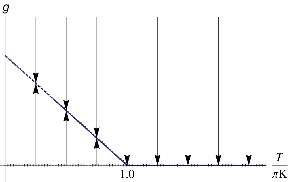
As illustrated in Fig. 7, decays to the fixed line for and grows to a
| (129) |
fixed line for . Thus, we find that the 2D cell exhibits a Cardy-Ostlund-like [40] phase transition at
| (130) |
between a high-temperature phase, where at long scales surface pinning is smoothed away by thermal fluctuations and a low-temperature glassy pinned phase, controlled by the nontrivial fixed line. This surface-pinned state (and the associated transition) is quite similar to the super-rough phase of a crystal surface grown on a random substrate [38], to the 1+1 vortex glass phase of flux-line vortices (confined to a plane) in type-II superconductors [4, 20, 41], and to the 3D smectic liquid crystals pinned by a random porous environment of e.g., aerogel [7].
One key distinction here is the irrelevance in 2D of the tilt pinning potential [37]
| (131) |
in contrast to its relevance in these other bulk pinning systems [4, 38, 20, 41, 7], where it leads to a super-rough phase characterized by roughness. This difference leads to a distinct behavior of correlation functions in the pinned phase for the surface-pinning problem. Because this 2D case is somewhat academic, with our main focus on the experimentally relevant 3D cell, we do not explore it any further here.
IV.1.2 Finite-thickness cell
We now focus on the behavior of a finite thickness cell with Dirichlet or Neumann boundary conditions on the top homogeneous substrate. Much of the RG analysis of the previous section extends to this case after substitutions of and , Eqs. (113) and (118), respectively, for . With these changes the rescalings Eqs. (106) and (107) are supplemented with the exact flow equation for the cell thickness
| (132) |
The zero-temperature flow equation takes the same form as for an infinite cell, with ,
| (133) |
except that the constant is replaced by -dependent functions , , given by
| (134a) | |||||
| (134b) | |||||
for the two boundary conditions on the top substrate. The dimensionless disorder variance functions in Eqs. (134a) and (134b) have been, respectively, defined by
| (135a) | |||||
| (135b) | |||||
The limiting cases of these flow equations can be easily understood. For a thick cell equations for both (top substrate) boundary conditions reduce to an infinite cell analyzed in the previous section. In the opposite extreme of a microscopically thin cell, such that , the functions reduce to
| (136a) | |||||
| (136b) | |||||
corresponding to flow equations for a ()-dimensional bulk random-field model, which in the case of the Dirichlet boundary condition is in a uniform external field. In this Dirichlet case, the eigenvalue is negative for any physical dimension, showing that random pinning is always dominated by an ordering field of the rubbed top substrate. In contrast, in the Neumann case, the flow as expected is identical to that of a () bulk system with the eigenvalue of .
For a more realistic situation of a finite cell thickness , there is a crossover from an infinite -dimensional cell limit at small such that to an effective ()-dimensional system for . The corresponding crossover scale is given by . An independent crossover scale encoded in flow equations, Eq. (133) is set by a scale at which the nonlinear terms become comparable to the linear ones, where the flow leaves the vicinity of the Gaussian fixed point and (in the bulk system, i.e., for ) would approach the nontrivial fixed point (122). From the flow equations, Eq. (133), one can see that this latter scale is simply set by the Larkin length, with .
As we discuss below, the detailed nature of distortions strongly depends on the relative size of these two crossover scales and on the type of boundary condition on the homogeneous substrate. We naturally designate the two cases, and , as thin and thick cells, respectively.
IV.2 Correlation function
We now turn to a calculation of correlation functions. As discussed earlier, on short scales (smaller than the Larkin length), these can be simply computed using the random-torque model of Sec. III. However, as we have seen in Sec. IV.1, for the effective pinning becomes strong (compared to the elastic energy) on scales longer than the Larkin length, leading to a breakdown of the perturbative expansion and of the random-torque model. Nevertheless, we can utilize the above FRG, which effectively allows us to treat pinning nonperturbatively to overcome this difficulty. To see this, we note that the power of the renormalization group is that it establishes a connection between a correlation function at a small wave vector (which is impossible to calculate in perturbation theory due to the aforementioned infra-red divergences) to the same correlation function at large wave vectors (short scales), which can be easily calculated in a controlled perturbation theory [42, 14, 38, 7].
This relation for the Fourier transform of the surface () correlation function is given by
where the prefactor on the right-hand side comes from the dimensional rescalings of Sec. IV.1, remembering the momentum-conserving function in the definition of , and for simplicity we chose to keep fixed under rescaling. We then choose the rescaling variable such that
| (138) |
which allows us to reexpress on the right hand side of Eq. () in terms of the wave vector
Because the correlation function on the right-hand side is evaluated at the large wave vector, it is easily computed perturbatively in a weak pinning potential if the latter is indeed small at long scale , i.e., the pinning is weak. To lowest order, the computation can be done with the replicated random-torque (Larkin) surface model
| (140) | |||||
which gives
where in the last line we neglected the subdominant thermal part. To evaluate the resulting correlation function
| (142) |
explicitly requires an analysis of the flow for specific boundary conditions.
IV.2.1 Infinitely thick cell:
We first focus on an infinitely thick cell, for which the above correlation function reduces to
where in the second line we used Eq. (120) to express the result in terms of the dimensionless disorder variance.
(i) . As we learned in the previous section, for this range of dimensions, at large [which by Eq. (138) corresponds to small ], the dimensionless pinning variance flows to a fixed point (122), giving
| (144) |
as presented in Sec. I.
We can now use this result to compute real-space correlations on in-plane scales , characterized for by
| (145) | |||||
In above, is a (nearly) -independent contribution to the correlation function from short scales, , where Larkin approximation [random-torque model, Eq. (56), from Sec. III] is valid and is given by (see Appendix C.2)
with the generalized incomplete gamma function and is the Euler’s constant. In contrast to its small () behavior, Eq. (III.2), is -independent for and is plotted in Fig. 8.


The second long-scale part, in Eq. (145) is a universal contribution [determined by the fixed point function, Eq. (122)], that for and low temperatures (when 2D effects discussed in Sec. IV.1 can be neglected) can be straightforwardly computed. It is compactly given by (see Appendix C.3)
| (149) | |||||
and is plotted in Fig. 9.

(ii) . For a three-dimensional (infinite-thick) cell the pinning is marginally irrelevant, with the large solution given by Eq. (126). Using this inside Eq. (), we obtain
| (150) |
The short-scale part, , is similar to Eq. (IV.2.1), which when evaluated in 3D reduces to (see Appendix C.2)
where , plotted in Fig. 11, is again nearly -independent for , as the only -dependence enters through , which averages to zero for these large wave vectors with .
For , the long-scale universal part in Eq. (145) is obtained directly from the fixed-point function (126) [21, 22], derived in Appendix C.3, and it is given by
and is plotted in Fig. 12.
Thus on the substrate, at long length scales and for a thick 3D cell, we find
| (158) | |||||
as claimed in the Sec. I and first found in Ref. [21]. The complete 3D correlation function is plotted in Fig. 13.
We conclude this section with a computation of the surface orientational order parameter,
| (159) | |||||
where somewhat crudely we approximated it by assuming Gaussian correlations in . This order parameter is of particular interest to the application of our results to a finite-thickness cell with a Dirichlet or a Neumann boundary condition imposed on the homogeneous substrate (see Fig. 1).
Because, as we have seen above [see, e.g., Eqs.(82) and (158)], in the limit of an infinitely thick cell () grows without bound with system size , the orientational order parameter vanishes in the thermodynamic limit. For a more realistic situation of a finite cell, the decay of orientational order is determined by the cell thickness, , and the nature of the boundary conditions on the homogeneous substrate.


IV.2.2 Crossover in a Dirichlet cell
Contrasting the bulk behavior, for a cell with a Dirichlet (homogeneous) substrate, we expect the growth of root-mean fluctuations of to be suppressed by the alignment by this homogeneous substrate. Thus, in this case, is nonzero and the orientational order is stable for an arbitrarily thick (but finite) cell.
We can analyze by estimating using the results of FRG found in Sec. IV.1. To this end, we examine the asymptotics of the FRG flow in Eqs. (132) and (133). For a thin cell (defined by ), reaches the microscopic scale at and therefore before . Since beyond , , pinning is irrelevant and the flow is cut-off at scale , scales beyond are not probed (the flow never leaves the vicinity of the Gaussian fixed point), and can be accurately computed within the Larkin approximation (random-torque model), cut-off by .
In contrast, for a thick cell (defined by ), the flow crosses over to the vicinity of the nontrivial fixed point (leaves the Gaussian fixed point) before it is cut-off by the finite . In this case, on longer scales, , the fluctuations are cut-off by (by the flow’s return to the Gaussian fixed point). In this thick cell regime, is thus given by the matching calculation of Sec. IV.2 with the diverging () dependence cutoff by .
Following this crossover allows us to calculate . For a thin cell, and , we have
| (160) | |||||
where we used the Larkin approximation Eq. (60) together with Eq. (51), valid for since the Dirichlet flow in Eq. (133) never leaves the vicinity of the Gaussian fixed point.
For a thick cell and , we have
| (161) | |||||
where we neglected the subdominant contribution from scales longer than (where the RG flow for “turns around” heading back toward the Gaussian fixed, i.e., pinning is irrelevant), in the first term of the second line approximated the correlator by its fixed-point value (144), valid for (such that the flow approaches the vicinity of the nontrivial fixed point), and approximated in the second term by its Gaussian fixed point expression (Larkin approximation), valid for . We also used the definition of to approximate the second term in the last line by .
Repeating above estimates for , for a thin cell (), we find
| (162) | |||||
and for a thick cell (),
where we employed the same asymptotic approximations as for .
Putting these crossovers together, we finally obtain the surface orientational order parameter for thin and thick cells in ,
and in 3D
| (170) |
where , are universal exponents [given in Eqs. (161) and ()] and is a nonuniversal constant. The 3D surface order parameter for such Dirichlet cell of thickness is illustrated in Fig. 2.
IV.2.3 Crossover in a Neumann cell
Above analysis straightforwardly extends to a finite-thickness cell with the Neumann boundary condition on the homogeneous substrate. At long scales, a finite-thickness Neumann cell reduces to an effective “film,” i.e., a -dimensional bulk random-field model. Thus, we expect the disordering effect of the random pinning to be enhanced compared to the system, where additional homogeneous bulk degrees of freedom have a stabilizing effect against pinning ( reduced from down to ).
This is reflected in the behavior of both the correlators in the random-torque model [given by Eqs. (52) and (60)], and in the FRG flow that becomes only more divergent on scales , as . Hence, in contrast to the Dirichlet cell (where finite suppresses the effect of the random potential), in a Neumann cell, finite thickness enhances the effects of random surface pinning. Consequently, independent of the Neumann cell thickness, the orientational order parameter, , vanishes for .
V Strong pinning limit
In all of the above analysis, we focused on the most interesting weak surface disorder, where pinning is collective, dominating over the elastic energy only on the macroscopic length scales, longer than . This assumption is what justified our treatment of the elastic energy as dominant (at least on short scales, smaller than ), allowing an expansion about the ordered (nematic) state. However, it is quite possible that in some (e.g., liquid crystal) applications, it is the opposite limit of strong pinning that is of interest.
In the latter strong-disorder limit, the surface-pinning potential (by definition) dominates over the elastic energy at all, even microscopic scales, with . To treat this regime, we instead perturb in the elastic energy about a random ground state, , that exactly minimizes the random pinning potential . That is, . We then expand about this random ground state, obtaining
where . A minimization of the above Hamiltonian then straightforwardly gives
| (172) |
From this analysis we can readily identifying a strong-coupling pinning length
| (173) | |||||
which is a scale below which the -order parameter no longer faithfully follows spatial variations of the local random potential and thus it is a strong-coupling version of the Larkin length. In above, we restored the pinning potential correlation length to also account for the more realistic case where is distinct and longer than the microscopic molecular cutoff scale . Hence we conclude that below the pinning correlation length , there is a crossover from weak to strong pinning limit when the (weak-coupling) Larkin length, , drops down to . On these shorter scales, the collective pinning analysis of previous sections and corresponding results break down.
VI Application to liquid crystal cells
As discussed in the Sec. I, liquid crystal cells provided a strong motivation for our study of the orientational order in the presence of surface random pinning. However, although there is a qualitative overlap, in detail a model of a surface-pinned liquid crystal cell, a priori can be quite different from a basic model studied above. Furthermore, the detailed model very much depends on the specific nature of the liquid crystal phase and thus requires an extensive study that lies beyond the current paper. However, to put our above results for an model in a physical context, we now briefly examine a formulation of a surface-pinning problem for real liquid crystals, focusing on nematic and smectic phases, deferring their detailed analysis to a future study.
VI.1 Nematic liquid crystal phase
The key distinction of the nematic liquid crystal phase as compared to the model studied so far is the nature of the Goldstone modes, that for a nematic is given by a three-dimensional unit vector (strictly speaking with opposite ends identified forming an manifold), the nematic director
| (174) |
as opposed to its -model counterpart, where it is a single azimuthal (planar) angle, , with the polar angle fixed at zero by some easy-plane anisotropy. We note that in above, we chose a somewhat nonstandard (but here convenient for treating parallel surface alignment) convention for . We also implicitly ignored the difficult question of topological defects proliferation and the corresponding stability of the elastic glass. If indeed important, for weak disorder, we expect their effects to set in on much longer length scales, thereby providing a wide intermediate range of scales, where defect-free model is of interest.
In the nematic phase, the bulk energy of a nematic director is described by the well-known Frank-Oseen expression [43]
| (175) | |||||
Within a simplifying one-elastic-constant approximation, , and together with the surface-pinning energy and polar parameterization, Eq. (174), the above equation gives the elastic Hamiltonian for the nematic surface-pinned cell
| (176) | |||||
where the surface-pinning energy
| (177) | |||||
is given by a purely homogeneous planar () alignment on the top () substrate and a planar alignment with a heterogeneous azimuthal component on the bottom () substrate. The latter is encoded in a random pinning function with a periodicity of , presented in Sec. II, with capturing the symmetry of the nematic liquid crystal phase.
For a thin cell and weak random pinning on the bottom substrate, such that the scale of is much smaller than , clearly the planar alignment, while of random strength (on the bottom substrate), remains planar on both substrates. We further note that because (computed within the -model approximation) remains finite in the physically interesting dimensions (i.e., infrared convergent for ) and small for weak pinning (decaying into the bulk with ), based on Fredericks transition phenomenology [43], we do not expect planar surface alignment by to be overturned by a weak second term in Eq. (176).
Thus, with the exception of small regions (that are rare for weak disorder), is the solution that minimizes the total energy. With this, the nematic cell model reduces to the surface random-field model for the director’s azimuthal orientation , studied above [21, 22]. Hence, for weak pinning, all of -model results detailed above apply directly to a nematic liquid crystal cell.
In contrast, we expect strong pinning to lead to large azimuthal distortions that will be accompanied by big variations both on the random substrate and in the bulk. For intermediate pinning strength, the system can perhaps even exhibit a random Fredericks-like transition corresponding to a bulk escape from a planar surface configuration, driven by a large . We leave the detailed study of the associated subtleties for this system, which distinguish it from the simple model to a future research.
VI.2 Smectic liquid crystal phase
Another important realization of a random surface-pinning problem is that of a smectic liquid crystal on a heterogeneous substrate, as for example realized in recent experiments [26] mentioned in the Sec. I. We will focus on the experimentally and theoretically more interesting case of the bookshelf geometry, illustrated in Fig. 1, where layers and director are, respectively, perpendicular and parallel to the substrate. Choosing the coordinate system as indicated in Fig. 14, so that the smectic layers lie parallel to the plane, with the average layer normal along the axis and the random substrate located at and running perpendicular the axis, the total energy is given by
| (178) | |||||
where the first two terms describe the usual smectic elasticity, with bending and compressional elastic constants and (for simplicity taken to be harmonic [44]), and the last term is a surface-pinning energy given by
where for convenience we defined and extended its to dimensions transverse to .

In above, the and terms are the homogeneous and random components of the orientational pinning [ inducing a homogeneous parallel to the surface director alignment and capturing random azimuthal director pinning within the heterogeneous substrate plane] and is the positional pinning of surface layers with the random substrate [6, 7]. In getting to the final form we expanded about its pinning-free orientation along and used the smectic “Higgs mechanism” [43, 7] to make a replacement , valid inside a smectic phase.
Following procedure used for the model, this randomly surface-pinned smectic model can be used to analyze the phenomenology of a smectic liquid crystal cell with the hopes of understanding long-scale random textures observed in Ref. [26]. Because (as illustrated above) the smectic elasticity and pinning differ qualitatively from that of an model, we expect a phenomenology that is qualitatively distinct from that found for the simple model and the nematic phase found above. We leave the interesting and nontrivial study of a random smectic cell to a future research.
VI.3 Experimental observables
One attractive feature of liquid crystals is that their orientational order can be readily studied via light microscopy. In its simplest form, the technique utilizes a crossed polarizer-analyzer pair on the front and back of a cell, typically transversely oriented. In this geometry, the spatial (within the plane) distribution of the transmitted light intensity through the cell is sensitive to the azimuthal variation of the local optic axis and therefore measures the director’s planar spatial distribution.
For a fully ordered planar nematic state, with a uniform director orientation at an azimuthal angle with respect to the polarizer (or analyzer), the transmitted light intensity through a uniaxial cell of thickness is given by [43]
| (180) |
In above, is the phase difference between ordinary and extraordinary components of light with wavelength , respectively, characterized by , indices of refraction. In the simplest case of the director uniformly aligned along the polarizer () or the analyzer (), this leads to a uniformly vanishing transmitted light intensity. Conversely, the maximum light transmission is produced for a uniform director orientation relative to the polarizer (or equivalently, transversely-crossed analyzer). The last factor in Eq. (180) leads to transmission color selectivity with optical anisotropy and cell thickness.
For a spatially nonuniform director variation, the analysis of the transmitted light intensity is more complicated. However, for a nematic variation on a scale longer than light’s transverse coherent length (a typical situation for illumination with incoherent source), the output intensity simply images the transverse (-) optic axis variation, with each coherence region treatable as an independent column of depth . Furthermore, in the limit that spatial variation along is also smooth on the scale of light’s wavelength, the transmission through each column can be treated in Mauguin limit, where light components along and perpendicular to the optic axes simply adiabatically follow the local director orientation .
For a -crossed polarizer-analyzer pair, standard analysis in this Mauguin limit then gives the output light intensity (behind the analyzer, at )
| (181) | |||||
For the director on the back substrate aligned (by the Dirichlet boundary conditions) with the polarizer axis (and perpendicular to the analyzer), i.e., , the output signal simplifies considerably to
| (182) |
and is thus directly related to the local surface orientational order parameter, studied in this paper. For example, a spatially averaged transmission through a Dirichlet cell is given by
| (183) | |||||
in which is computed in Eqs. (IV.2.2) and (170). Thus, for this choice of geometry, a thin Dirichlet cell has the expected vanishing transmission, that grows with cell thickness to its maximum value of . More stringent tests of our predictions can further be made by comparing (-) spatial correlations of light transmission, , with orientational correlation functions to which these are clearly directly related according to
An even more direct probe of director correlations is possible through the polarized confocal microscopy [45], where an image of the local director orientation at each depth can be produced. A numerical computation of thereby measured director correlation functions therefore allows a detailed comparison to results predicted here.
VII Summary and Conclusion
In this paper, we have studied the stability of random distortions in an model perturbed by a random surface pinning and discussed our findings in the context of nematic liquid crystal cell with a dirty non-rubbed substrate. We found that for a thick 3D cell, at long scales, the disordering effects of the random substrate always marginally dominate over the bulk nematic order. Thus, a 3D nematic order is marginally unstable with orientational “roughness” growing as on long scales. We have also extended these results to a finite-thickness cell, with a second homogeneous substrate with parallel Dirichlet and Neumann boundary conditions. Not surprisingly, in the former case, the nematic order is stabilized to arbitrary long scales, but with the nematic order parameter (and the corresponding birefringence) exhibiting a crossover from a large value for a thin (weakly heterogeneous) cell to a small value for a thick (strongly heterogeneous) cell at a characteristic cell thickness set by the Larkin length, . We expect our predictions to be experimentally testable via a polarizer-analyzer transmission microscopy and by studying how the nematic order is recovered in response to a tunable in-plane aligning electric or magnetic field. We propose that the predicted statistical properties (correlation functions) of the random substrate-induced director textures can be quantitatively tested with the polarized confocal microscopy [45].
VIII Acknowledgments
We thank N. Clark, V. Gurarie, M. Hermele, I. Smalyukh, and S. Todari for discussions and acknowledge financial support by the National Science Foundation through Grants No. DMR-0321848 and No. MRSEC DMR-0820579 (L.R., Q.Z.) and the Berkeley Miller and the University of Colorado Faculty Fellowships (L.R.). L.R. thanks Berkeley Physics Department for its hospitality during part of this work.
Appendix A Larkin lengths analysis
In this appendix, we provide the details for the analysis of the Larkin length [9] in finite thickness, two- and three-dimensional cells. As derived in Sec. III, the Larkin length is defined in the standard way, given by
| (185) |
with the ’s given by Eqs. (50)-(52) and the lower momentum cutoff of the integration given by . In the limit of an infinitely thick () cell above integral is straightforwardly computed, in 2D () giving
| (186) | |||||
which leads to a Larkin length
| (187) |
with the superscript denoting the result of an infinitely thick cell (that for simplicity of notation we will drop).
In 3D, with the two-dimensional random substrate, we obtain
| (188) | |||||
which gives the Larkin length as
| (189) |
For a general dimension , we have
| (190) | |||||
giving
| (191) |
where we ignored the strongly subdominant (for ) term.
A.1 Finite thickness in two dimensions
For a finite-thickness () 2D Dirichlet cell, the surface variance determines the Larkin length according to
| (192) | |||||
By scaling variables, this defines an implicit expression
| (193) |
for the Dirichlet Larkin length in terms of the infinite cell’s Larkin scale , latter simply a characterization of disorder given by Eq. (187).
Similarly for a 2D Neumann cell, we have
| (194) | |||||
which gives
| (195) |
both evaluated numerically and plotted in Fig. 6.
A.2 Finite thickness in three dimensions
Repeating the analysis in 3D for the Dirichlet cell, with scaled ultraviolet cutoff and
| (196) | |||||
gives
| (197) |
which reduces to
| (198) |
To get to this final result, we used the fact that the second integral in Eq. (197) is finite in the ultraviolet, for giving an -independent constant about , thereby eliminating dependence on .
A.3 Larkin length crossover
As we can see from Eqs. (193), (195), (198) and (199), the Larkin length in a cell of thickness depends on a single dimensionless ratio, , of the infinite cell Larkin length (characterizing pinning strength) to the cell thickness. We expect that for a thick cell (), the result of infinite thick cell should be recovered. On the other hand, for thin cells (), we expect the homogeneous substrate boundary condition to play a role. Namely, since the Dirichlet boundary condition on the top homogeneous substrate explicitly orders the director, suppressing the distortions of , we expect to diverge for a thin Dirichlet cell. Furthermore, since the Neumann boundary condition eliminates the stiffening by the bulk, in the thin Neumann cell we expect to approach the value for a -dimensional bulk system with -dimensional pinning. The expected crossover is indeed confirmed by a numerical evaluation with the solution illustrated in Fig. 6, with the Dirichlet diverging at in 2D and in 3D.
The divergent asymptotic behavior can be obtained by expanding the implicit expression for in Eqs. (193) and (198) around . For , we have
| (200) |
which making use of as reduces to
| (201) |
with
| (202) |
For , using as , we have
| (203) |
with
| (204) |
This leads to
| (205) |
quoted in the main text and consistent with the numerical evaluation of the integral solution.
Appendix B The cusp and the fixed point
For completeness, we now fill in some of the details (previously reviewed in Ref. [46]) for the RG evolution of the random potential variance into its universal cusped form. To this end, by differentiating the flow equation (121) for with respect to , we obtain
| (206) | |||||
Setting to , we obtain
| (207) | |||||
We note that is an even function and moreover (before the cusp develops) is smooth in , with .
Clearly, the flows of and are exact, with the later diverging in a finite RG time according to [11]
| (208) |
with . For a special case ( in our system with surface pinning), the cusp develops according to
| (209) |


Thus after a finite RG time , diverges, signaling the appearance of a cusp in , as illustrated in Fig. 15.
Appendix C Details of asymptotics of various correlation functions
As derived in the main text, in an infinitely thick cell, the momentum space correlation function has short- and long-scale limits. The former one, computed in the random-torque (Larkin) approximation (scale shorter than ) on the random substrate (), is given by
| (210) |
In the long-scale limit (small ), derived via FRG and matching methods in Sec.IV.2 it is instead given by
| (211) |
A Fourier transform of [using above limits and generalized to finite ; see Eqs. (45)-(47)] then gives this correlation function in real space.
C.1 Mean-squared distortion in Larkin approximation
The mean-squared distortion of can be given as
| (212) |
For , we have (with )
| (213) | |||||
in which the integral converges at large so we can ignore the upper cutoff of and the definition of as in Eq. (3) was used. Expanding this result at different range of values, we obtain
| (214) |
in which is the Euler’s constant.
For , we have
| (215) | |||||
making use of and the definition of as in Eq. (3). For different range of values, we obtain
| (216) |
Similarly, for , we need to consider the upper cutoff of and have
where . The mean-squared distortions for and are plotted in Fig. 5.
C.2 Correlation function in Larkin approximation
The short scales (where Larkin approximation holds) contribution to the real-space correlation is given by Eq. (). In an infinite thick cell, we have
| (221) |
in which the integral of has lower cutoff and upper cutoff . For simplicity of notation, we will ignore the superscript .
For and , since the kernel is convergent at large , we can extend the integral to infinity (requiring ) and obtain
| (222) | |||||
On the heterogeneous substrate (), we have
| (223) | |||||
where is the sine integral function. Making use of the expansion of at , for finite we obtain
| (224) | |||||
where the last approximation is taken for and the other terms are subdominant.
When , the oscillates strongly giving subdominant contribution. Then we have
in which the generalized incomplete gamma function and we made use of expansions at small () and at large ().
For and , we can extend the integral to infinity (requiring ) and obtain
| (229) | |||||
in which is the average of over a surface of a -dimension unit sphere. The correlation function could be evaluated numerically and on the heterogeneous substrate this result approaches (with )
| (230) | |||||
as given in Sec. III. Making use of the expansion at , we can evaluate the correlation function at finite as
| (231) | |||||
in which the last approximation is taken for and the other subdominant terms are ignored.
When , the again oscillates at the full range of and obtain
where we made use of expansions at small () and at large ().
For , the variables and are two dimensional, thus we have
| (236) | |||||
in which is the Bessel function of the first kind. The behavior of its correlation could be evaluated numerically and the asymptotics can be obtained approximately for different regions.
On the heterogeneous surface (), for small (), we have with and with , so in this region we have
| (237) | |||||
Making use of the expansion of , we can evaluate the correlation function at finite as
| (238) | |||||
where in the last approximation we kept the leading term for .
When , the expression simplifies to
in which we made use of expansions at small () and at large ().
C.3 Universal (long-scales) part of correlation function
The correlation function in momentum space at small () is obtained by FRG and matching methods in Sec. IV.2. Here we calculate the corresponding real-space correlation functions. By construction, this form of only holds at , with therefore entering as the upper (UV) cutoff on all integrals done here.
For , the FRG derived correlation function rated at is given by
A better approximation is obtained by using a “soft” upper cutoff by inserting a factor of inside above integrand.
For , this correlation function is given by
| (243) | |||||
where is system size to be taken to at the end of calculation. Using the gamma function expansion , we obtain
| (244) | |||||
Except for approximations associating with the matching method, this real-space result is an excellent approximation to a numerical integration of , as shown in Fig. 9. On the heterogeneous substrate and for , it reduces to .
For , the correlation function is given by
| (245) | |||||
which we evaluated numerically with a soft cutoff and plotted in Fig. 12.
Approximate asymptotic behavior of this correlation function can be obtained analytically
in which .
On the heterogeneous substrate (), the first integral is negligible, thus for we have
| (247) | |||||
Further away from the substrate such that , the acts like upper cutoff at , giving
| (248) | |||||
Finally, for , we find
| (249) | |||||
with numerical prefactor that is off by a factor of relative to the numerical integration that gives , as given in Sec. IV.2.
References
- [1] D. S. Fisher, G. M. Grinstein, and A. Khurana, Phys. Today 41(12), 56 (1988).
- [2] M. Mezard, G. Parisi, and M. A. Virasaro, Spin Glass Theory and Beyond (World Scientific, Singapore, 1987); K. Binder and A. P. Young, Rev. of Mod. Phys. 58, 801(1986).
- [3] Charge Density Waves in Solids, edited by L. P. Gorkov and G. Gruner (Elsevier, Amsterdam, 1989).
- [4] D. S. Fisher, M. P. A. Fisher, and D. A. Huse, Phys. Rev. B 43, 130 (1991)
- [5] M. Chan et al., Phys. Today 49(8), 30 (1996).
- [6] L. Radzihovsky and J. Toner, Phys. Rev. Lett. 79, 4214 (1997).
- [7] L. Radzihovsky and J. Toner, Phys. Rev. B 60, 206 (1999).
- [8] T. Bellini, L. Radzihovsky, J. Toner, and N. A. Clark, Science 294(5544), 1074 (2001).
- [9] A. Larkin, Sov. Phys. JETP 31, 784 (1970).
- [10] A. I. Larkin and Y. N. Ovchinnikov, J. Low Temp. Phys. 34, 409 (1979).
- [11] D. S. Fisher, Phys. Rev. B 31, 7233 (1985).
- [12] T. Nattermann, Phys. Rev. Lett. 64, 2454 (1990).
- [13] L. Balents and D. S. Fisher, Phys. Rev. B 48, 5949 (1993).
- [14] T. Giamarchi and P. Le Doussal, Phys. Rev. Lett. 72, 1530 (1994); Phys. Rev. B 52, 1242 (1995).
- [15] P. Le Doussal and K. Wiese, Phys. Rev. E 79, 051105 (2009).
- [16] L. Balents and P. Le Doussal, Ann. Phys. 315, 213 (2005).
- [17] D. McNamara, A. A. Middleton, and C. Zeng, Phys. Rev. B 60, 10062 (1999).
- [18] T. Klein, I. Joumard, S. Blanchard, J. Marcus, R. Cubitt, T. Giamarchi, and P. Le Doussal, Nature (London) 413, 404 (2001).
- [19] S. R. Park, S. M. Choi, D. C. Dender, J. W. Lynn, and X. S. Ling, Phys. Rev. Lett. 91, 167003 (2003).
- [20] D. S. Fisher, Phys. Rev. Lett. 78, 1964 (1997).
- [21] D. E. Feldman and V. M. Vinokur, Phys. Rev. Lett. 89, 227204 (2002).
- [22] L. Radzihovsky and Q. Zhang, Phys. Rev. Lett. 103, 167802 (2009).
- [23] Defects in Liquid Crystals: Computer Simulations, Theory and Experiments, edited by O. D. Lavrentovich, P. Pasini, C. Zannoni, and S. Zumer (Erice, Sicily, Italy, 2000).
- [24] B. W. Lee, D. R. Link, and N. A. Clark, Liq. Cryst. 27, 501 (2000); B. W. Lee and N. A. Clark, Langmuir 14, 5495 (1998).
- [25] N. Aryasova, Yu. Reznikov, and V. Reshetnyak, Mol. Cryst. Liq. Cryst. 412, 351 (2004).
- [26] C. D. Jones and N. A. Clark, Bull. Am. Phys. Soc. 49, 307 (2004); http://flux.aps.org/meetings/ YR04/MAR04/baps/abs/S1420002.html
- [27] Throughout will refer to the dimension of the bulk in contact with a dimensional heterogeneous surface.
- [28] L.R. thanks Senthil for discussion on this point.
- [29] Y. Imry and S. K. Ma, Phys. Rev. Lett. 35, 1399 (1975).
- [30] L. Radzihovsky, Phys. Rev. B 73, 104504 (2006).
- [31] C. L. Kane and M. P. A. Fisher, Phys. Rev. B 46, 15233 (1992).
- [32] This is certainly the case for the long-scale asymptotics of correlation functions, dominated by the ground-state distortion induced by the quenched random heterogeneity.
- [33] N. Aryasova, Mol. Cryst. Liq. Cryst. 475, 73 (2007).
- [34] S. F. Edwards and P. W. Anderson, J. Phys. F: Met. Phys. 5, 965 (1975).
- [35] Because we are perturbing about an ordered state , which is not a minimum of the random potential, the lowest nontrivial term in the Taylor expansion of the random potential is linear in .
- [36] K. G. Wilson and J. Kogut, Phys. Rep. 12, 75 (1974).
- [37] An additional operator generated by the coarse-graining of , is irrelevant in the RG sense for , in contrast to its familiar bulk disorder counter-part.
- [38] J. Toner and D. P. DiVincenzo, Phys. Rev. B 41, 632 (1990).
- [39] R. Chitra, T. Giamarchi, and P. Le Doussal, Phys. Rev. B 59, 4058 (1999).
- [40] J. L. Cardy and S. Ostlund, Phys. Rev. B 25, 6899 (1982).
- [41] M. P. A. Fisher, Phys. Rev. Lett. 62, 1415 (1989).
- [42] D. R. Nelson and J. Rudnick, Phys. Rev. Lett. 35, 178 (1975); J. Rudnick and D. R. Nelson, Phys. Rev. B 13, 2208 (1976).
- [43] P. G. de Gennes and J. Prost, The physics of liquid crystals, 2nd ed. (Oxford, New York, 1995).
- [44] Ignoring for now Grinstein-Pelcovits nonlinear elasticity [47] (which is known to be important[6, 7, 8])
- [45] I. I. Smalyukh, Mol. Cryst. Liq. Cryst. 477, 23 (2007); I. I. Smalyukh, S. V. Shiyanovskii, and O. D. Lavrentovich, Chem. Phys. Lett. 336, 88 (2001).
- [46] K. J. Wiese and P. Le Doussal, Markov Processes Relat. Fields 13, 777(2007); e-print arXiv:cond-mat/0611346.
- [47] G. A. Grinstein and R. Pelcovits, Phys. Rev. Lett. 47, 856 (1981).