Exclusive double-diffractive production of open charm
in proton-proton and proton-antiproton collisions

Preprint:

R. Maciuła Email: rafal.maciula@ifj.edu.pl Affiliation: Institute of Nuclear Physics PAN, PL-31-342 Cracow, Poland R. S. Pasechnik Email: roman.pasechnik@fysast.uu.se Affiliation: High Energy Physics, Department of Physics and Astronomy, Uppsala University Box 535, SE-75121 Uppsala, Sweden A. Szczurek Email: antoni.szczurek@ifj.edu.pl Affiliation: Institute of Nuclear Physics PAN, PL-31-342 Cracow, Poland and
University of Rzeszów, PL-35-959 Rzeszów, Poland

August 24, 2026

Abstract

We calculate differential cross sections for exclusive double diffractive (EDD) production of open charm in proton-proton and proton-antiproton collisions. Sizeable cross sections are found. The EDD contribution constitutes about 1 % of the total inclusive cross section for open charm production. A few differential distributions are shown and discussed. The EDD contribution falls faster both with transverse momentum of the $c$ quark/antiquark and the $c\bar{c}$ invariant mass than in the inclusive case.

pacs

13.87.Ce,14.65.Dw

I Introduction

The open charm production is often considered as a flag reaction to test the gluon distributions in the nucleon. For the $c\bar{c}$ and $b\bar{b}$ production at high-energies the gluon-gluon fusion is assumed to be the dominant mechanism. This process was calculated in the NLO collinear [1] as well as in the $k_{t}$ -factorisation [2, 3, 4, 5] approaches by several authors. These analyses seem to report on missing strength¹¹ 1 The situation is often somewhat clouded by studying the uncertainty bands due to variation of renormalization and factorization scales. These analyses lead to rather broad uncertainty bands which prevent definite conclusions.. This suggests that other processes ignored so far should be carefully evaluated.

The number of potential contributions is not small. In the present paper we concentrate on exclusive double diffractive (EDD) mechanism, which was not considered so far for the $c\bar{c}$ production. The mechanism of the exclusive double-diffractive production of open charm is shown in Fig. 1.

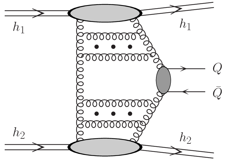
Refer to caption — Figure 1: The mechanism of exclusive double-diffractive production of open charm.

The EDD $b\bar{b}$ reaction consitutes a irreducible background to the exclusive Higgs boson production [6] measured in the $b\bar{b}$ channel. Up to now only approximate estimates of the $b\bar{b}$ production were presented in the literature. In the present paper we consider the $pp\to ppc\bar{c}$ reaction as a genuine 4-body process with exact kinematics which can be easily used with kinematical cuts. The amplitude of the genuine four-body reaction is written in analogy to the Kaidalov-Khoze-Martin-Ryskin (KKMR) approach used previously for the exclusive Higgs boson production [7, 8, 9].

II Matrix element and the cross section
for exclusive double diffractive $q\bar{q}$ pair production

Inclusive heavy quark/antiquark pair production was considered in detail, e.g. in Refs. [4, 5]. The nonrelativistic QCD methods were successfully applied also in the case of central exclusive production of heavy quarkonia in Refs. [10, 11, 12]. It looks quite natural to apply similar ideas to exclusive diffractive $q\bar{q}$ (unbound) pair production.

II.1 Kinematics

The kinematical variables for the process $pp\rightarrow p+\mathrm{``gap"}+(q\bar{q})+\mathrm{``gap"}+p$ are shown in Fig. 2.

We adopt here the following standard definition of the light cone coordinates

k^{+}\equiv n^{+}_{\alpha}k^{\alpha}=k^{0}+k^{3},\text{ }k^{-}\equiv n^{-}_{\alpha}k^{\alpha}=k^{0}-k^{3},\text{ }k_{t}=(0,k^{1},k^{2},0)=(0,{\bf k,}0{\bf)},

where $n^{\pm}$ are the light-cone basis vectors. In the c.m.s. frame

\displaystyle n^{+}=\frac{p_{2}}{E_{cms}},\qquad n^{-}=\frac{p_{1}}{E_{cms}},

(1)

and the momenta of the scattering hadrons are given by

p_{1}^{+}=p_{2}^{-}=\sqrt{s},\text{ \ }p_{1}^{-}=p_{2}^{+}=p_{1,t}=p_{2,t}=0,

with the Mandelstam variable $s=4E_{cms}^{2}.$

Within the standard $k_{t}$ -factorisation approach, the decomposition of gluon momenta into longitudinal and transverse parts in the high-energy limit is

	$\displaystyle q_{1}=x_{1}p_{1}+q_{1,t},\qquad q_{2}=x_{2}p_{2}+q_{2,t},\qquad 0<x_{1,2}<1,$		(2)
	$\displaystyle q_{0}=x^{\prime}_{1}p_{1}+x^{\prime}_{2}p_{2}+q_{0,t},\quad x^{\prime}_{1}\sim x^{\prime}_{2}\ll x_{1,2},\quad q_{0,1,2}^{2}\simeq q_{0/1/2,t}^{2}.$

Making use of energy-momentum conservation laws

\displaystyle q_{1}=p_{1}-p^{\prime}_{1}-q_{0},\qquad q_{2}=p_{2}-p^{\prime}_{2}+q_{0},\qquad q_{1}+q_{2}=k_{1}+k_{2}

(3)

we write

\displaystyle s\,x_{1}x_{2}=M_{q\bar{q}}^{2}+|{\bf P}_{t}|^{2}\equiv M_{q\bar{q},\perp}^{2},\qquad M_{q\bar{q}}^{2}=(k_{1}+k_{2})^{2}\;,

(4)

where $M_{q\bar{q}}$ is the invariant mass of the $q\bar{q}$ pair, and ${\bf P}_{t}$ is its transverse 3-momentum.

II.2 The amplitude for $pp\to ppQ\bar{Q}$

Let us concentrate on the simplest case of production of $q\bar{q}$ pair in the color singlet state. Color octet state would demand an emission of an extra gluon [13] which considerably complicates the calculations, and we postpone such an analysis for future studies.

In analogy to the Kaidalov-Khoze-Martin-Ryskin approach (KKMR) [7, 8, 9] for Higgs boson production, we write the amplitude of the exclusive diffractive $q\bar{q}$ pair production $pp\to p(q\bar{q})p$ in the color singlet state as

	$\displaystyle{\cal M}_{\lambda_{q}\lambda_{\bar{q}}}^{pp\to ppq\bar{q}}(p^{\prime}_{1},p^{\prime}_{2},k_{1},k_{2})$	$\displaystyle=$	$\displaystyle s\cdot\pi^{2}\frac{1}{2}\frac{\delta_{c_{1}c_{2}}}{N_{c}^{2}-1}\,\Im\int d^{2}q_{0,t}\;V_{\lambda_{q}\lambda_{\bar{q}}}^{c_{1}c_{2}}(q_{1},q_{2},k_{1},k_{2})$		(5)
			$\displaystyle\frac{f^{\mathrm{off}}_{g,1}(x_{1},x_{1}^{\prime},q_{0,t}^{2},q_{1,t}^{2},t_{1})f^{\mathrm{off}}_{g,2}(x_{2},x_{2}^{\prime},q_{0,t}^{2},q_{2,t}^{2},t_{2})}{q_{0,t}^{2}\,q_{1,t}^{2}\,q_{2,t}^{2}}\;,$		(5)

where $\lambda_{q},\,\lambda_{\bar{q}}$ are helicities of heavy $q$ and $\bar{q}$ , respectively. Above $f_{1}^{\mathrm{off}}$ and $f_{2}^{\mathrm{off}}$ are the off-diagonal unintegrated gluon distributions in nucleon 1 and 2, respectively. They will be discussed in a separate subsection below.

The longitudinal momentum fractions of active gluons are calculated based on kinematical variables of outgoing quark and antiquark

	$\displaystyle x_{1}$	$\displaystyle=$	$\displaystyle\frac{m_{3,t}}{\sqrt{s}}\exp(+y_{3})+\frac{m_{4,t}}{\sqrt{s}}\exp(+y_{4})\;,$
	$\displaystyle x_{2}$	$\displaystyle=$	$\displaystyle\frac{m_{3,t}}{\sqrt{s}}\exp(-y_{3})+\frac{m_{4,t}}{\sqrt{s}}\exp(-y_{4})\;,$		(6)

where $m_{3,t}$ and $m_{4,t}$ are transverse masses of the quark and antiquark, respectively, and $y_{3}$ and $y_{4}$ are corresponding rapidities.

The bare amplitude above is subjected to absorption corrections which, in general, depend on collision energy and on the spin-parity of the produced central system [11]. We shall discuss this issue shortly when presenting our results.

II.3 $gg\to Q\bar{Q}$ vertex

Let us consider the subprocess amplitude for the $q\bar{q}$ pair production via off-shell gluon-gluon fusion. The vertex factor $V_{\lambda_{q}\lambda_{\bar{q}}}^{c_{1}c_{2}}=V_{\lambda_{q}\lambda_{\bar{q}}}^{c_{1}c_{2}}(q_{1},q_{2},k_{1},k_{2})$ in expression (5) is the production amplitude of a pair of massive quark $q$ and antiquark $\bar{q}$ with helicities $\lambda_{q}$ , $\lambda_{\bar{q}}$ and momenta $k_{1}$ , $k_{2}$ , respectively. Within the QMRK approach [14], the color singlet $q\bar{q}$ pair production amplitude can be written as

	$\displaystyle V_{\lambda_{q}\lambda_{\bar{q}}}^{c_{1}c_{2}}(q_{1},q_{2},k_{1},k_{2})\equiv n^{+}_{\mu}n^{-}_{\nu}V_{\lambda_{q}\lambda_{\bar{q}}}^{c_{1}c_{2},\,\mu\nu}(q_{1},q_{2},k_{1},k_{2}),$		(7)
	$\displaystyle V_{\lambda_{q}\lambda_{\bar{q}}}^{c_{1}c_{2},\,\mu\nu}(q_{1},q_{2},k_{1},k_{2})=-g^{2}\sum_{i,k}\left\langle 3i,\bar{3}k\|1\right\rangle\times$
	$\displaystyle\bar{u}_{\lambda_{q}}(k_{1})(t^{c_{1}}_{ij}t^{c_{2}}_{jk}b^{\mu\nu}(q_{1},q_{2},k_{1},k_{2})-t^{c_{2}}_{kj}t^{c_{1}}_{ji}\bar{b}^{\mu\nu}(q_{1},q_{2},k_{1},k_{2}))v_{\lambda_{\bar{q}}}(k_{2}),$

where $t^{c}$ are the color group generators in the fundamental representation, $u(k_{1})$ and $v(k_{2})$ are on-shell quark and antiquark spinors, respectively, $b,\,\bar{b}$ are vertices (8) arising from the Feynman rules :

	$\displaystyle b^{\mu\nu}(q_{1},q_{2},k_{1},k_{2})=\gamma^{\nu}\frac{\hat{q}_{1}-\hat{k}_{1}-m}{(q_{1}-k_{1})^{2}-m^{2}}\gamma^{\mu}\;,$		(8)
	$\displaystyle\bar{b}^{\mu\nu}(q_{1},q_{2},k_{1},k_{2})=\gamma^{\mu}\frac{\hat{q}_{1}-\hat{k}_{2}+m}{(q_{1}-k_{2})^{2}-m^{2}}\gamma^{\nu}\;.$

The SU(3) Clebsch-Gordan coefficient $\left\langle 3i,\bar{3}k|1\right\rangle=\delta^{ik}/\sqrt{N_{c}}$ in Eq. (7) projects out the color quantum numbers of the $q\bar{q}$ pair onto the color singlet state. Factor $1/\sqrt{N_{c}}$ provides the averaging of the matrix element squared over intermediate color states of quarks.

The tensorial part of the amplitude is therefore:

	$\displaystyle{}V_{\lambda_{q}\lambda_{\bar{q}}}^{\mu\nu}(q_{1},q_{2},k_{1},k_{2})=g_{s}^{2}\,\bar{u}_{\lambda_{q}}(k_{1})\biggl(\gamma^{\nu}\frac{\hat{q}_{1}-\hat{k}_{1}-m}{(q_{1}-k_{1})^{2}-m^{2}}\gamma^{\mu}-\gamma^{\mu}\frac{\hat{q}_{1}-\hat{k}_{2}+m}{(q_{1}-k_{2})^{2}-m^{2}}\gamma^{\nu}\biggr)v_{\lambda_{\bar{q}}}(k_{2}).$
			(9)

Taking into account definitions (1) and momentum conservation (2) and using the gauge invariance properties we get the following projection to the light cone vectors (so called “Gribov’s trick”)

$\displaystyle V_{\lambda_{q}\lambda_{\bar{q}}}^{c_{1}c_{2}}(q_{1},q_{2},k_{1},k_{2})$	$\displaystyle=$	$\displaystyle n^{+}_{\mu}n^{-}_{\nu}V_{\lambda_{q}\lambda_{\bar{q}},\,\mu\nu}^{c_{1}c_{2}}(q_{1},q_{2},k_{1},k_{2})$	(10)
	$\displaystyle=$	$\displaystyle\frac{4}{s}\frac{q^{\nu}_{1}-q^{\nu}_{1,t}}{x_{1}}\frac{q^{\mu}_{2}-q^{\mu}_{2,t}}{x_{2}}V^{c_{1}c_{2}}_{\lambda_{q}\lambda_{\bar{q}},\,\mu\nu}(q_{1},q_{2},k_{1},k_{2})$
	$\displaystyle=$	$\displaystyle\frac{4}{s}\frac{q^{\nu}_{1,t}}{x_{1}}\frac{q^{\mu}_{2,t}}{x_{2}}V^{c_{1}c_{2}}_{\lambda_{q}\lambda_{\bar{q}},\,\mu\nu}(q_{1},q_{2},k_{1},k_{2}).$

Using (9) and (10) we can write

	$\displaystyle V_{\lambda_{q}\lambda_{\bar{q}}}^{c_{1}c_{2}}(q_{1},q_{2},k_{1},k_{2})=\frac{4}{sx_{1}x_{2}}g_{s}^{2}\,\bar{u}_{\lambda_{q}}(k_{1})\biggl(\hat{q}_{1t}\frac{\hat{q}_{1}-\hat{k}_{1}-m}{(q_{1}-k_{1})^{2}-m^{2}}\hat{q}_{2t}-\hat{q}_{2t}\frac{\hat{q}_{1}-\hat{k}_{2}+m}{(q_{1}-k_{2})^{2}-m^{2}}\hat{q}_{1t}\biggr)v_{\lambda_{\bar{q}}}(k_{2}).$
			(11)

The coupling constants $g_{s}^{2}\to g_{s}(\mu_{r,1}^{2})g_{s}(\mu_{r,2}^{2})$ . In the present calculation we take the renormalization scale to be $\mu_{r,1}^{2}=\mu_{r,2}^{2}=M_{q\bar{q}}^{2}/4$ . The matrix element (11) is then calculated numerically. Inserting it to Eq. (5) we can calculate numerically the whole amplitude for the $pp\to ppQ\bar{Q}$ process.

II.4 Off-diagonal unintegrated gluon distributions

In the KMR approach the off-diagonal parton distributions are calculated as

$\displaystyle f_{1}^{\mathrm{KMR}}(x_{1},Q_{1,t}^{2},\mu^{2},t_{1})$	$\displaystyle=$	$\displaystyle R_{g}\frac{d[g(x_{1},k_{t}^{2})S_{1/2}(k_{t}^{2},\mu^{2})]}{d\log k_{t}^{2}}\|_{k_{t}^{2}=Q_{1t}^{2}}\;F(t_{1})\;$
	$\displaystyle\approx$	$\displaystyle R_{g}\frac{dg(x_{1},k_{t}^{2})}{d\log k_{t}^{2}}\|_{k_{t}^{2}=Q_{1,t}^{2}}\;S_{1/2}(Q_{1,t}^{2},\mu^{2})\;F(t_{1})\;,$
$\displaystyle f_{2}^{\mathrm{KMR}}(x_{2},Q_{2,t}^{2},\mu^{2},t_{2})$	$\displaystyle=$	$\displaystyle R_{g}\frac{d[g(x_{2},k_{t}^{2})S_{1/2}(k_{t}^{2},\mu^{2})]}{d\log k_{t}^{2}}\|_{k_{t}^{2}=Q_{2t}^{2}}\;F(t_{2})\;$
	$\displaystyle\approx$	$\displaystyle R_{g}\frac{dg(x_{2},k_{t}^{2})}{d\log k_{t}^{2}}\|_{k_{t}^{2}=Q_{2,t}^{2}}\;S_{1/2}(Q_{2,t}^{2},\mu^{2})\;F(t_{2})\;,$

where $S_{1/2}(q_{t}^{2},\mu^{2})$ is a Sudakov-like form factor relevant for the case under consideration [17]. The last approximate(!) equalities come from the fact that in the region under consideration the Sudakov-like form factors are somewhat slower functions of transverse momenta than the collinear gluon distributions. While reasonable for an estimate of gluon distribution it may be not sufficient for precise calculation of the cross section. It is reasonable to take a running (factorization) scale as: $\mu_{1}^{2}=\mu_{2}^{2}=M_{q\bar{q}}^{2}/4$ . We shall call the formulae () as the DDT-like formulae [18], for brevity.

The factor $R_{g}$ here cannot be calculated from first principles in the most general case of off-diagonal UGDFs. It can be estimated in the case of off-diagonal collinear PDFs when $x^{\prime}\ll x$ and $xg=x^{-\lambda}(1-x)^{n}$ [20]. Then

R_{g}=\frac{2^{2\lambda+3}}{\sqrt{\pi}}\frac{\Gamma(\lambda+5/2)}{\Gamma(\lambda+4)}\;.

(13)

In a more realistic case of DGLAP GDF $\lambda=\lambda(x,\mu^{2})$ . Typically $R_{g}\sim$ 1.3 – 1.4 at Tevatron energy. A more general case of unintegrated off-diagonal distributions was discussed in Ref. [17], but we will not touch them here.

The off-diagonal form factors are parametrized here as:

F(t)=\exp\left(B_{\mathrm{off}}t\right)\;.

(14)

In practical calculations in this letter we take $B_{\mathrm{off}}$ = 2 GeV^-2.

In the original KMR approach the following prescription for the effective transverse momentum is taken:

	$\displaystyle Q_{1,t}^{2}$	$\displaystyle=$	$\displaystyle\min\left(q_{0,t}^{2},q_{1,t}^{2}\right)\;,$
	$\displaystyle Q_{2,t}^{2}$	$\displaystyle=$	$\displaystyle\min\left(q_{0,t}^{2},q_{2,t}^{2}\right)\;.$		(15)

Other prescriptions are also possible [10].

In evaluating $f_{1}$ and $f_{2}$ needed for calculating the amplitude (5) we use the GRV collinear distributions [16].

It was proposed [17] to express the $S_{1/2}$ form factors in Eq. () through the standard Sudakov form factors as:

S_{1/2}(q_{t}^{2},\mu^{2})=\sqrt{T_{g}(q_{t}^{2},\mu^{2})}\;.

(16)

The Sudakov form factor, a two-dimensional function $T_{g}(q_{t}^{2},\mu^{2})$ as a function of transverse momentum squared $q_{t}^{2}$ and a log₁₀ of the scale parameter $\mu^{2}$ , is shown in Fig. 3.

A strong dependence on $\mu^{2}$ ( $\log_{10}(\mu^{2})$ in the figure) is clearly visible. This dependence leads to a huge perturbative damping of the off-diagonal UGDFs (and, as a consequence, of the amplitude and the cross section) in the case when objects $X$ with sizeable masses ( $M_{X}$ ) are produced, i.e. when $\mu^{2}\sim M_{X}^{2}$ .

II.5 The $pp\to ppQ\bar{Q}$ cross section

The cross section is obtained by assuming a general $2\to 4$ reaction:

d\sigma=\frac{1}{2s}|{\cal M}_{2\to 4}|^{2}(2\pi)^{4}\delta^{4}(p_{a}+p_{b}-p_{1}-p_{2}-p_{3}-p_{4})\frac{d^{3}p_{1}}{(2\pi)^{3}2E_{1}}\frac{d^{3}p_{2}}{(2\pi)^{3}2E_{2}}\frac{d^{3}p_{3}}{(2\pi)^{3}2E_{3}}\frac{d^{3}p_{4}}{(2\pi)^{3}2E_{4}}\;.

(17)

The details how to conveniently reduce the number of kinematical integration variables are given elsewhere [19].

III Results

As for the exclusive production of $\chi_{c}$ mesons [11, 12], in the case when the KMR UGDFs are used an extra cut-off on transverse momenta is applied i.e. the formula (5) is used if

	$\displaystyle Q_{1,t}^{2}$	$\displaystyle=$	$\displaystyle\min(q_{0,t}^{2},q_{1,t}^{2})>Q_{t,cut}^{2}\;,$
	$\displaystyle Q_{2,t}^{2}$	$\displaystyle=$	$\displaystyle\min(q_{0,t}^{2},q_{2,t}^{2})>Q_{t,cut}^{2}\;.$		(18)

Otherwise the cross section is set to zero.

Let us proceed now with the presentation of differential distributions of charm quarks produced in the EDD mechanism. In our calculation here we fix the scale of the Sudakov form factor to be $\mu=M_{c\bar{c}}/2$ . Such a choice of the scale leads to a strong damping of the situations with large rapidity gaps between $c$ and $\bar{c}$ ²² 2 Large rapidity gap means automatically large invariant mass $M_{c\bar{c}}$ of the $c\bar{c}$ system..

In Fig. 4 we show distribution in rapidity. The results obtained with the KMR method are shown together with inclusive gluon-gluon contribution calculated as in Ref. [5]. The effect of absorption leads to a damping of the cross section by an energy-dependent factor. For the Tevatron this factor is about 0.1. If the extra factor is taken into account the EDD contribution is of the order of 1% of the dominant gluon-gluon fusion contribution.

The corresponding rapidity-integrated cross sections are: 6.6 $\mu$ b for exact DDT formula, 2.4 $\mu$ b for simplified DDT formula (see Eq. ()). For comparison the inclusive cross section (gluon-gluon component only) is 807 $\mu$ b.

In Fig. 5 we show the differential cross section in transverse momentum of the charm quark. Compared to the inclusive case, the exclusive contribution falls significantly faster with transverse momentum than in the inclusive case.

In Fig. 6 we show the distribution in the invariant mass of $c$ and $\bar{c}$ . The fluctuations visible in the figure are due to the fact that the integration is not directly in $M_{c\bar{c}}$ , but in other variables, and the number of integration points is rather restricted. Compared to the inclusive case the invariant mass distribution for the EDD component is significantly steeper. This is due to the Sudakov-like form factor which, according to the procedure described above, damps the cross section for large invariant masses $M_{X}$ .

As in the inclusive case within the $k_{t}$ -factorisation approach [5] the $c\bar{c}$ pair possesses the transverse momentum different from zero. The corresponding distribution is shown in Fig. 7. The distribution for the exclusive case (the two lower lines) is much narrower compared to the inclusive case (the upper line).

IV Conclusions

In the present letter we have evaluated, for the first time in the literature, the contribution of exclusive-double diffractive production of open charm. We have found a sizeable cross sections of the order of 1 % of the standard inclusive gluon-gluon fusion contribution at the Tevatron energy. The details depend, however, on the UGDFs used in the evaluation of the cross section. The most reliable estimate is obtained with the KMR off-diagonal UGDFs. These distributions were verified recently in the production of $\chi_{c}$ quarkonia [11, 12], i.e. for the kinematics similar to the present one.

It would be therefore very valuable to measure the diffractive mechanism discussed in the present paper. How to identify the EDD contribution? The events corresponding to the EDD contribution are expected to be related to a rather small multiplicity of particles (mainly pions or kaons) associated with $c$ or $\bar{c}$ , or more precisely charmed mesons which are formed in the process of hadronization of charm quarks into charmed mesons. One method would be therefore to measure $D$ mesons with a trigger on small pion multiplicity. Another method would be to measure $D$ mesons in association with rapidity gaps with respect to the outgoing protons/antiprotons. This is partially possible at the Tevatron and will be accessible at the LHC as well.

Acknowledgments

We are indebted to Ch. Royon for an interesting discussion. Useful discussions with Gunnar Ingelman and Oleg Teryaev are gratefully acknowledged. This study was partially supported by the Polish grant of MNiSW N N202 249235.

References

[1] P. Nason, S. Dawson and R.K. Ellis, Nucl. Phys. B303 (1988) 607;
G. Altarelli, M. Diemoz, G. Martinelli and P. Nason, Nucl. Phys. B308 (1988) 724;
P. Nason, S. Dawson and R.K. Ellis, Nucl. Phys. B327 (1989) 49;
W. Beenakker, H. Kuijf, W.L. Van Neerven and J. Smith, Phys. Rev. D40 (1989) 54.
[2] S. Catani, M. Ciafaloni and F. Hautmann, Nucl. Phys. 366 (1991) 135;
J.C. Collins and R.K. Ellis, Nucl. Phys. B360 (1991) 3;
R.D. Ball and R.K. Ellis, J.H.E.P. 0105 (2001) 053.
[3] S.P. Baranov and M. Smizanska, Phys. Rev. D62 (2000) 014012.
[4] P. Hagler, R. Kirschner, A. Schafer, L. Szymanowski and O. Teryaev, Phys. Rev. D 62, 071502 (2000) [arXiv:hep-ph/0002077].
[5] M. Łuszczak and A. Szczurek, Phys. Rev. D73 (2006) 054028.
[6] A. De. Roeck et al., Eur. Phys. J. C25 (2002) 391;
S. Heinemeyer et al., Eur. Phys. J. C53 (2008) 231;
A. G. Shuvaev, V. A. Khoze, A. D. Martin and M. G. Ryskin, Eur. Phys. J. C 56, 467 (2008) [arXiv:0806.1447 [hep-ph]].
[7] V.A. Khoze, A.D. Martin and M.G. Ryskin, Phys. Lett. B 401, 330 (1997);
V.A. Khoze, A.D. Martin and M.G. Ryskin, Eur. Phys. J. C 23, 311 (2002).
[8] A.B. Kaidalov, V.A. Khoze, A.D. Martin and M.G. Ryskin, Eur. Phys. J. C 33, 261 (2004).
[9] A.B. Kaidalov, V.A. Khoze, A.D. Martin and M.G. Ryskin, Eur. Phys. J. C 31, 387 (2003) [arXiv:hep-ph/0307064].
[10] R. S. Pasechnik, A. Szczurek and O. V. Teryaev, Phys. Rev. D 78, 014007 (2008) [arXiv:0709.0857 [hep-ph]];
R. S. Pasechnik, A. Szczurek and O. V. Teryaev, Phys. Lett. B 680, 62 (2009) [arXiv:0901.4187 [hep-ph]].
[11] L.A. Harland-Lang, V.A. Khoze, M.G. Ryskin and W.J. Stirling, arXiv:0909.4748.
[12] R. Pasechnik, A. Szczurek and O.V. Teryaev, arXiv:0912.4251[hep-ph].
[13] V. A. Khoze, M. G. Ryskin and A. D. Martin, Eur. Phys. J. C 64, 361 (2009) [arXiv:0907.0966 [hep-ph]].
[14] V. S. Fadin and L. N. Lipatov, Nucl. Phys. B 477, 767 (1996) [arXiv:hep-ph/9602287].
[15] P. Hagler, R. Kirschner, A. Schafer, L. Szymanowski and O. V. Teryaev, Phys. Rev. Lett. 86, 1446 (2001) [arXiv:hep-ph/0004263].
[16] M. Glück, E. Reya and A. Vogt, Z. Phys. C67 (1995) 433.
[17] A. D. Martin and M. G. Ryskin, Phys. Rev. D 64, 094017 (2001) [arXiv:hep-ph/0107149].
[18] Yu.L. Dokshitzer, D.I. Dyakonov and S.I. Troyan, Phys. Rep. 58 (1980) 269.
[19] P. Lebiedowicz and A. Szczurek, arXiv:0912.0190[hep-ph].
[20] A.G. Shuvaev et al., Phys. Rev. D60 (1999) 014015.

Exclusive double-diffractive production of open charm in proton-proton and proton-antiproton collisions