Asymptotic independence for unimodal densities
Abstract
Asymptotic independence of the components of random vectors is a concept used in many applications. The standard criteria for checking asymptotic independence are given in terms of distribution functions (dfs). Dfs are rarely available in an explicit form, especially in the multivariate case. Often we are given the form of the density or, via the shape of the data clouds, one can obtain a good geometric image of the asymptotic shape of the level sets of the density. This paper establishes a simple sufficient condition for asymptotic independence for light-tailed densities in terms of this asymptotic shape. This condition extends Sibuya’s classic result on asymptotic independence for Gaussian densities.
Key words: Asymptotic independence; blunt; homothetic density; level set; skew-normal; star-shaped 2000 MSC: 60G55, 60G70, 62E20
1 Introduction
The purpose of the present paper is to provide simple sufficient conditions that ensure asymptotic independence of the components of random vectors whose probability distribution is described by a density. Standard criteria for checking asymptotic independence are given in terms of distribution functions (dfs). However, these are not always available in an explicit form in the multivariate case, and they give little insight in what large samples from a distribution will look like. Often we are given a density in analytic form. For light-tailed densities, the data clouds give a good geometric image of the asymptotic shape of the level sets. Hence it is of interest to have conditions for asymptotic independence in terms of the shape of the level sets of the underlying density, or in terms of a limiting shape for data clouds.
For vector valued data it is standard practice to plot the bivariate sample clouds for all component pairs. In our final result it is the asymptotic behaviour of the shape of these bivariate sample clouds, as the size of the data set increases, that determines asymptotic independence of the coordinates for the underlying multivariate distribution.
Unimodal densities whose level sets all have the same shape are called homothetic. The decay along any ray then is the same up to a scale constant depending on the direction, and hence the concept of light and heavy tails is well-defined. This remains true if we only assume that the level sets have the same shape asymptotically. Our primary focus here is on light-tailed densities, but for additional insight we also include some results for the heavy-tailed case. Throughout the paper, we assume continuity of dfs and of densities.
Intuitively, for bivariate data, asymptotic independence means that large values in one coordinate are unlikely to be accompanied by large values in the other coordinate. Situations with a low chance of simultaneous extremes are often encountered in practice, for example in applications which involve modeling environmental data (e.g. [17]) or network traffic data (e.g. [19]); see [25] for further references. It is a well-known result, dating back to 1959 (see [26]), that the components of a vector with a Gaussian density are asymptotically independent whatever the correlation. Asymptotic independence also holds for light-tailed elliptical densities (see e.g. [15]). As a further generalization we shall show that a vector with a continuously differentiable homothetic light-tailed density whose level sets are convex has asymptotically independent components.
Theorem 1.1.
Let be a bounded open convex set in , containing the origin, with a boundary (i.e., at each boundary point there is a unique tangent plane). Let decrease to zero such that and let be positive reals such that . If is a random vector in with a continuous probability density whose level sets satisfy
| (1.1) |
then the components of are asymptotically independent.
We shall prove more general results, Theorem 3.10 and 3.11 below. The generalizations we introduce are simple, but they result in theorems for which some extra terminology has to be developed.
- •
- •
Asymptotic independence holds if it holds for the bivariate marginals; in this spirit, our theorem imposes conditions on the projection of the set on the -coordinate plane.
- •
Convex level sets are replaced by star-shaped level sets.
- •
The condition of a smooth () boundary is replaced by a condition which only affects the maximum: the coordinatewise supremum of the points in should not be a boundary point of . Such a set is called blunt.
- •
Our final result (Theorem 4.3) is on bivariate sample clouds. If these converge onto a blunt star-shaped set, asymptotic independence holds.
The conditions in Theorem 1.1 above on the sequences and ensure that the density has light tails. If then the density has heavy tails, and the same condition on the shape of the level sets implies asymptotic dependence.
The paper is organized as follows. In Section 2 we discuss the concept of asymptotic independence. Section 3 introduces the class of continuous multivariate homothetic densities with star-shaped level sets. The simple structure of these densities makes them a good starting point in our investigation of the relation between the shape of the level sets and asymptotic independence. Here we formulate our main results (Theorem 3.10 and 3.11) for light-tailed densities, and a counterpart (Theorem 3.12) for heavy-tailed densities. In Section 4 we introduce sample clouds, and state conditions for asymptotic independence in terms of their limiting shape (Theorem 4.3). Section 5 provides various examples. The appendix clears up a number of minor points in the main text, by providing supplementary results and counterexamples.
2 Asymptotic independence
In this section we discuss asymptotic independence for multivariate distributions. We begin with a heuristic approach in the bivariate setting. This will clarify the significance of the concept for risk management. We discuss the commonly used criteria for asymptotic independence, the relation with multivariate extreme value theory, and describe possible forms of asymptotic dependence.
2.1 Heuristics
In finance one is interested in the future value of stocks, say in one year’s time. Let and denote the future value of two stocks. Suppose the distribution of the pair is given by a df with continuous marginals and . One is concerned about the risk that the stocks have a low value at this future date. Let denote the -quantile of the first stock, , and the -quantile of the second. The probability that the values of both stocks lie below the -quantile for some given small value of is . A risk averse investor would like this probability (of simultaneous loss) to be small compared to the probability of a loss in either of the stocks. Future extreme low values of the two stocks are said to be asymptotically independent if for . Asymptotic dependence will increase risk for a portfolio containing these two stocks.
A different example of risk is presented by the yearly maxima for high water levels at particular points on the coast of Holland, Great Britain and the U.S., say IJmuiden, Harwich and New Orleans. Consider a data set of 200 observations stretching back to the beginning of the nineteenth century. We assume that the data have been standardized to offset tidal effects. Now for each of these locations pick the five largest values. This yields three subsets of five elements in the set of 200 years. One would suppose that there is considerable overlap between the five years selected for IJmuiden and for Harwich, since in both cases the cause is the same, a North Western storm in the North Atlantic forcing water into the funnel formed by the West coast of Holland and Belgium and the South coast of Great Britain, and opening into the Southern Atlantic via the Channel. High water levels in New Orleans have a different cause. So sea levels in New Orleans and in IJmuiden should be asymptotically independent, and one would expect the corresponding five point subsets to be disjoint with high probability. In general, given a positive integer and a sequence of independent observations from a bivariate df , one could look in the sample cloud of the first points at the largest observations for the coordinate and for the coordinate . This yields two subsets of the index set . Let denote the probability that the two subsets have a point in common. In the case of asymptotic independence one would expect that for fixed , as . This is indeed the case, as shown in [12] (Proposition 2).
A related way to understand extremal dependence is by looking at the probability of a record, , the probability that the coordinatewise maximum of a sample of points is given by one of the sample points. It is shown in [13] (Theorem 2) that this probability vanishes as exactly when the underlying vector has asymptotically independent components. For the sake of completeness we give an alternative proof of this basic result in the Appendix; see Proposition A.1.
2.2 Sibuya’s condition
In his seminal paper [26] on multivariate extremes, Sibuya shows that the components of bivariate vectors with normal densities, whatever their correlation, are asymptotically independent. For a vector with df and continuous marginals and he introduces a function by
| (2.2) |
The function is well-defined and continuous on the unit square. We can now give Sibuya’s condition for asymptotic independence (see Theorem 2 in [26]).
Definition Let have df with continuous marginals. The components and are asymptotically independent if the function introduced above satisfies
| (2.3) |
By abuse of language we also say that the vector or the df is asymptotically independent.
Independence of a bivariate vector is not affected by the marginal distributions. Similarly for asymptotic independence. It is preserved under coordinatewise increasing transformations. Since we assume that the marginals and are continuous, there is a unique function on the unit square such that . The function is known as the copula of the df . It is a df on the unit square with uniform marginals. Sibuya’s condition is a condition on the copula since for . If the condition holds for a vector with a continuous df , it automatically holds for any vector whose df is continuous and has the same copula as .
In this paper we consider asymptotic independence for maxima. For minima one would define asymptotic independence similarly, in terms of the copula, by: for .
Proposition 2.1.
Suppose there exist such that
| (2.4) |
Then asymptotic independence holds, and the relation (2.4) is valid for all .
Proof We may assume by symmetry and replacing by in the denominator. By monotonicity Sibuya’s condition holds. A similar argument gives (2.4) for any positive . 
For a vector with marginal dfs and , Sibuya’s condition may be formulated in terms of conditional quantile exceedances as
| (2.5) |
where for denotes the (minimal) -quantile of . The limit , if it exists, is known as the upper tail dependence coefficient. So and are asymptotically independent if and only if their upper tail dependence coefficient is zero.
Sibuya’s condition is simple, but the formulation in terms of survival probabilities is inconvenient. The quantiles in (2.5) may be hard to determine since this amounts to computing the inverse of the dfs. There is a simple criterium in terms of sums:
Proposition 2.2.
Let have a df with continuous marginals and , and let . If then and are asymptotically independent.
Proof Sibuya’s function satisfies . This gives Sibuya’s condition (2.3). 
Below we give criteria in terms of continuous curves , , for which and tend to one as .
Proposition 2.3.
Let have df with continuous marginals and . The components and are asymptotically independent if and only if for any there exists a continuous curve , , such that is positive and vanishes for for , and such that
| (2.6) |
Proof Assume asymptotic independence. One may choose and continuous and increasing such that for all . Then (2.3) gives (2.6). Now assume (2.6). Let where . By symmetry we may assume . Then
This holds for all . So Sibuya’s condition is satisfied. 
Asymptotic independence is preserved under quite severe deformations of the distribution.
Corollary 2.4.
Let be a convex open cone in and let and be probability densities which are positive on , vanish off and for which the quotients and are bounded on . Let have density and let have density . If and are asymptotically independent, then so are and .
Proof The inequality implies by integration that the same inequalities hold for the univariate and bivariate marginal densities and tail functions. So . Similarly the inequality gives an inequality with the constant for the tail probabilities: for . Now use (2.6) for to establish the same relation for . The extra factor has no effect in the limit. 
The concept of asymptotic independence has been refined by looking at the rate at which vanishes for , or more generally by looking at the behaviour of the survival function for . See [25] or [23]. This second order theory is called hidden regular variation. We shall not treat this subject in our paper. Since our interest is in multivariate densities rather than dfs, we give conditions on the density which ensure asymptotic independence of the components. So the assumption of continuous dfs is not restrictive. We shall also assume that the densities are continuous on a convex cone and vanish outside this cone. In our context, this cone will typically be either the whole space or the open positive orthant .
2.3 Asymptotic independence and multivariate extreme value theory
Asymptotic independence has to do with extremes, more precisely with bivariate maxima. Knowledge of multivariate extreme value theory is not indispensable for understanding asymptotic independence, but it will help to better understand asymptotic dependence.
For multivariate extreme value theory we have to assume that each of the marginals of the multivariate df lies in the domain of attraction of a univariate extreme value limit law (see e.g. Section 0.3 in [24] for a definition). As above let with be independent observations from the bivariate df , and write for the th coordinatewise partial maximum. For simplicity assume the marginals are equal with the standard Fréchet df on . The normalized marginal maxima and again have the Fréchet df by the scaling property . The scaled bivariate maximum has df . Suppose converges weakly to a limit distribution , known as a multivariate extreme value distribution or a max-stable distribution. The limit vector lives on , and the components and have a Fréchet law. Asymptotic independence for the df is equivalent to independence of the components of the limit vector (see e.g. Proposition 5.27 in [24] or Theorem 6.2.3 in [8]).
The convergence becomes easier to handle if one takes logarithms. Write . Since is asymptotic to for we may write the limit relation as
| (2.7) |
The left hand side is a df of the measure , where is the probability distribution of the vector . So is the mean measure of the sample cloud and . Pointwise convergence on implies pointwise convergence on and vague convergence . One can prove weak convergence on for any . It follows that the scaled sample clouds converge in distribution to a Poisson point process on weakly on the complement of centered disks. The Poisson point process is of interest since it gives an asymptotic description of the large vectors in the sample cloud. Moreover, the coordinatewise maximum of the scaled sample cloud converges in distribution to the coordinatewise maximum of as the sample size goes to infinity.
Sibuya’s condition holds precisely if . (Indeed for , and the survival function satisfies by Sibuya’s condition and Proposition 2.1.) In this case the measure has density zero on the open quadrant by differentiation (see also Proposition 5.24 in [24]). So is the sum of two measures, one on the positive horizontal and one the positive vertical axis, both with density . The point process thus is the superposition of two Poisson point processes on these halfaxes, and the two point processes are independent since the halfaxes are disjoint. This yields a simple description of the behaviour of large sample clouds: Asymptotically there is no relation between very large observations in the horizontal direction, and very large observations in the vertical direction.
So far we have looked at asymptotic independence for bivariate distributions. Unlike independence, for a multivariate df asymptotic independence holds if it holds for the bivariate marginals; see e.g. Remark 6.2.5 in [8]. Here is the argument. For simplicity assume has standard Fréchet marginals, and the multivariate maxima converge in distribution. The scaled sample clouds then converge in distribution to a Poisson point process on with mean measure weakly on the complement of any centered ball. If Sibuya’s condition holds for the bivariate marginals, then the projection of on the -plane will live on the two positive halfaxes in this plane. It follows that lives on the set of points in which have at most one positive coordinate, the union of the positive halfaxes. The restrictions of to these halfaxes are independent (since the positive halfaxes are disjoint). Hence the multivariate extreme value limit vector has independent components.
2.4 Asymptotic dependence
Asymptotic dependence is an ambiguous term. Logically it means the absence of asymptotic independence. We shall usually interpret it in a more constructive manner to mean the existence of a max-stable limit law . This in turn implies convergence in distribution of the normalized sample clouds to a Poisson point process , whose mean measure has df , as sketched above. The tail dependence coefficient in (2.5) gives only a very restricted view of extremal dependence. As pointed out in Section 8.2 in [21], a positive coefficient does not imply that the underlying distribution belongs to the maximum domain of attraction of some extreme value limit law. The exponent measure provides a much more informative description of asymptotic dependence. Points of which do not lie on one of the axes denote a simultaneous occurrence of very large values in two or more coordinates in the corresponding point of the normalized sample. Thus the point process (or equivalently ) gives a complete description of how the extreme upper order statistics in the different coordinates are linked.
3 Densities and level sets
The aim of this section is to give conditions in terms of the density which will guarantee asymptotic independence. Two aspects of densities play an important role in our analysis: the shape of the level sets and the tail behaviour. We consider densities which are completely specified by just these two quantities - a shape for the level sets, and a decreasing function governing the rate of decay of the tails. In many cases of practical interest the shape is a bounded open convex set, containing the origin. The density then is continuous if and only if the decreasing function is. We shall also consider such unimodal densities which vanish outside the positive orthant.
3.1 Homothetic densities
Homothetic densities are densities whose level sets are scaled copies of a given open set :
| (3.8) |
We assume that is a bounded open star-shaped set. A star-shaped set has the property that with any point it contains all points for . Assume the set contains the origin. If each ray intersects the boundary in one point, then the set can be represented using a gauge function that satisfies (i) for , (homogeneity property), and (ii) . The conditions on the set and the continuity of ensure that the gauge function is continuous. If the set is convex, then so is the gauge function. If in addition the set is symmetric, , then the gauge function is a norm on , and the set is the open unit ball in this norm. For any bounded open star-shaped set the sets , , form an increasing family. Their union is an open cone. It is a proper cone if the origin is a boundary point of . One may then still define the gauge function . This now is a function on the open cone . It is continuous on the cone if each ray in the cone intersects the boundary of in a single point, see Proposition 3.2 below.
Gauge functions allow us to give analytic expressions for homothetic densities with the same ease with which one handles spherically symmetric densities. Continuous homothetic densities have the form for a decreasing continuous function on . This formula holds for all for which the ray through intersects the set .
Definition 1.
Let denote the class of all bounded open star-shaped sets , for which the cone is convex, and for which the gauge function is continuous on this cone. A density on belongs to the class if the shape belongs to the class , and if is of the form , where the density generator is decreasing, positive and continuous. We set outside the cone on which the gauge function is defined.
It is apparent from the above definition that densities in are (star) unimodal since all the level sets , are star-shaped; cf. Section 2.2 in [9]. Typical examples of densities in to keep in mind are the multivariate centered normal densities and, more generally, elliptically symmetric densities, discussed for example in [10]. See also Example A.1. In certain applications, elliptical symmetry may be too restrictive. Densities in give the flexibility to model directional irregularities present in the data clouds, and to handle distributions on the positive orthant. The regularity conditions exclude pathological sets; see Example A.2.
Before we proceed by looking at properties of these densities, let us review some related classes of models proposed in the literature. The -spherical densities ([22]) extend the class of spherical densities by allowing level sets to be balls in -norm for any . A further generalization is given by so-called -spherical densities ([11]), where the scale function plays the same role as the gauge function defined above. In fact, our class is a subclass of the -spherical densities in that we restrict level sets to be bounded and star-shaped, and to be continuous on . In a recent paper [1], the authors advocate to study densities in terms of their contours.
For a given shape , what conditions does the density generator have to satisfy in order that the function is a probability density on ? By regarding the set below the graph of as a pile of thin -shaped slices we obtain the following partial integration result:
| (3.9) |
Observing that and letting tend to infinity, we obtain the condition (cf. Equation (5) in [11]): .
The class of unimodal densities introduced above is invariant under linear transformations. If the vector has density then the vector has density , where is the image of the star-shaped (convex) set under the linear transformation , and hence is also star-shaped (convex). A nice illustration of this invariance is the extension of spherical distributions to elliptical ones.
For densities in the distinction between light and heavy tails is crucial for asymptotic independence. It is determined by the behaviour of the generator at infinity. Let us recall the definitions of regular and rapid variation.
Definition 2.
A measurable function is regularly varying at with exponent , if for
| (3.10) |
if , then is called slowly varying; is rapidly varying at if
| (3.11) |
If the generator of a density varies rapidly, the density has light tails. In our terminology has light tails precisely if is continuous, positive, and strictly decreasing on , and if there is a strictly increasing sequence such that and .
Rapid variation of allows us to give strong inequalities for the measure with density .
Proposition 3.1.
Let have density with a rapidly varying density generator .
- (i)
For any
(3.12) - (ii)
For any non-empty open set
(3.13)
Proof Rapid variation implies that eventually for , and hence the rings , , have measure . The rings are disjoint, and their union is the complement of . On summing the odd and the even terms we find with :
This gives (3.12). The integral over a thin ring is much larger than the integral over the set outside the ring. Formally, take and to obtain (3.12). To prove (3.13) take a non-empty open subset whose closure lies in . Then if is small, and hence by rapid variation of as above the infimum of over is much larger than the supremum of over the ring . Since is a constant we conclude that , and (3.13) follows from (3.12). 
We now give some extra details on star-shaped sets.
Proposition 3.2.
Let be a bounded open star-shaped set. Suppose for each non-zero vector there is one positive real such that lies on the boundary of . Then the gauge function is continuous on the cone .
Proof Let denote an open unit ball. If contains the origin, it contains a ball , and by homogeneity on . So the gauge function then is continuous in the origin. Now suppose it is discontinuous in a point outside the origin. We may assume that and that there is a sequence such that and . Let be close to . Then , and implies eventually, hence and so since is arbitrary. This implies eventually, and this also holds for for . Hence is a boundary point. But so is . This contradicts our assumption on the boundary of . 
In general densities in are not closed under projection, even if is convex. If a random vector has density , then the density of need not be homothetic, and the univariate marginals need not even be unimodal; see Example A.3. There are some exceptions. Projections of spherical densities are spherical, and if the level sets are balls in for some then this also holds for projections along the coordinate axes. The class itself is closed under projection. If is a bounded open convex set containing the origin, then so is the vertical projection of onto the horizontal hyperplane; if the origin is a boundary point of it may be an interior point of .
Proposition 3.3.
Suppose . Let be the vertical projection of onto the horizontal hyperplane. Then .
Proof Write to distinguish the horizontal and vertical part of the vector . It is clear that is a bounded open star-shaped set. Moreover is the projection of the cone , and hence an open convex cone. We have to prove continuity of the gauge function on . If is not continuous, there exists a vector and a sequence such that and because is open. Hence for all and there exist such that . Since is bounded, the sequence is bounded, and we may assume that it converges to some element . Then , and continuity of implies . Contradiction. 
3.2 Densities whose level sets are asymptotically star-shaped
In this section we relax the condition that all level sets have the same shape to the condition that the level sets, properly scaled, converge to a set . We restrict attention to the light-tailed setting.
Definition 3.
Let . A positive probability density on belongs to the set if there exist sequences and with and such that for any eventually
| (3.14) |
We write . A continuous positive function is shape equivalent to if its level sets satisfy (3.14).
The sequences and determine a set of continuous decreasing functions which satisfy . All these functions vary slowly for by the assumption that and . It is this set of slowly varying functions rather than the particular sequences and which are of interest.
Proposition 3.4.
If the slowly varying function above is strictly decreasing, defined on for some , and vanishes in , then the inverse function is a continuous positive strictly decreasing function on which varies rapidly in , and is shape equivalent to , and for all
| (3.15) |
Proof Rapid variation of the inverse function follows from Theorem 2.4.7(i) in [6]. Shape equivalence holds since and by assumption. 
Since one may take a strictly increasing subsequence such that the asymptotic equality remains valid. Take . Any continuous strictly decreasing function on which vanishes in and has the value in satisfies the conditions of the proposition above. So there are many continuous strictly decreasing functions on which vary rapidly in such that is shape equivalent to .
For functions in the inequalities in Proposition 3.1 also hold. Moreover, they have the nice property that the marginals of will lie in , where is the projection of on the th coordinate.
Lemma 3.5.
Let . Let for denote the measure with density for a fixed non-zero vector . Then for any open set which intersects
| (3.16) |
Proof Let be shape equivalent to and define to have density . It suffices to prove (3.16) for the measures with density . Let be a non-empty open subset of which lies in the complement of for some , and whose closure lies in . For we may apply the pointwise inequality (3.17) below and conclude that , where we choose so small that . Then, using (3.13), and another application of the pointwise inequality gives (3.16). 
Proposition 3.6.
Suppose has density . Let be a non-zero linear combination of the components of . Then has a density where is the open interval .
Proof We may assume that is the vertical coordinate. The condition for implies by integration over horizontal hyperplanes for . This gives rapid variation. The thin tails of ensure that is continuous. Let . We claim that the average of over and over , say and , is much larger than over both and , say and , as . It suffices to show that and are much larger than . This follows from (3.16) since the horizontal slice contains the open set , and is much larger than . A similar argument holds for the strip . Let lie between and . Then on and holds off . Hence holds for small for sufficiently large . 
It is not known whether a similar result holds for the bivariate marginals of .
One can also define shape equivalence for functions with heavy tails. In that case shape equivalence is the same as asymptotic equality in infinity, see Proposition A.2. For light tails the behaviour of the quotient of two shape equivalent functions may be very erratic. Example A.4 in the Appendix exhibits some functions which are shape equivalent to the bivariate Gaussian density.
The level set inequalities in (3.15) imply the pointwise inequalities:
| (3.17) |
This shows that a function is shape equivalent to for and if for every
| (3.18) |
Rapid variation implies that the left side goes to and the right to . Hence we find:
Proposition 3.7.
is shape equivalent to if is positive and is bounded.
For Weibull-like functions of the form where for a continuous strictly increasing function which varies regularly with positive exponent there is a simple alternative description of shape equivalence.
Lemma 3.8.
Suppose where is continuous, strictly increasing and varies regularly in with exponent . Then varies rapidly in and is shape equivalent to if and only if holds for all sequences .
Proof Regular variation of gives and for . The claim then follows from (3.18) with . 
Proposition 3.9.
Suppose is a continuous positive density on . Let there exist a function on which is positive outside a bounded set and a non-zero vector such that
| (3.19) |
Then there exists a set containing the origin, a positive constant such that , and a continuous strictly increasing function on which varies regularly with exponent in such that is asymptotic to in , and is shape equivalent to where .
Proof Set . Then varies regularly in with exponent . For any unit vector the function varies regularly in since has a positive limit for and . Uniform convergence on compact sets implies that is continuous on the unit sphere, and implies . This proves that , and for since (3.19) implies uniform convergence on compact sets, and is continuous and hence bounded on compact sets. Hence and (3.19) with gives and continuity of implies . Set . Then . Let . Then varies regularly with exponent , and we may choose positive, continuous and strictly increasing and asymptotic to this function for . Then gives for . Lemma 3.8 then shows that is shape equivalent to and since varies rapidly if varies regularly with exponent it follows that . 
3.3 Criteria for asymptotic independence
A random vector with a spherically symmetric density will have asymptotically independent components if the generator varies rapidly, and it will have asymptotically dependent components if varies regularly (see e.g. Theorem 4.3 in [15], or Proposition 3.2 in [14]). These results remain valid for where denotes the open unit ball. One may replace by certain bounded open star-shaped sets , as will be shown in Theorem 3.11 and 3.12 below.
With any bounded open set one may associate the open intervals , , obtained by projecting onto the th coordinate. Then is the smallest open box containing , and is the coordinatewise supremum of all points in (and ).
Asymptotic independence depends on the bivariate marginal distributions. Hence we introduce the projections of on the coordinates. For we denote by the projection of onto the two-dimensional space spanned by the unit base vectors and . The sets lie in by Proposition 3.3, and fits exactly into the rectangle . The cone generated by is the projection of the cone generated by .
Definition 4.
The set is blunt if the point does not lie in the closure of .
A bounded open convex set in is smooth in the boundary point if there is a unique hyperplane which contains but which does not intersect , the tangent plane to at . For a planar set this means that is not a vertex. If the convex hull of is smooth in all points then all bivariate projections are blunt.
We can now state our main results for asymptotic independence in terms of densities.
Theorem 3.10.
If has a light-tailed homothetic density , and is convex with a smooth boundary, then for any two distinct unit vector and the random variables and are asymptotically independent. The result remains valid if the density of is in .
Proof First assume and are linearly independent. Introduce new coordinates such that and become the first two base vectors and . It suffices to check that the assumption holds for vertical tangent planes, hyperplanes which project onto a line in the two-dimensional -plane. The characterization of is geometrical and so it is preserved under linear transformations. The projection in the new coordinates is also convex and smooth. Hence is blunt, and we may apply Theorem 3.11 below. If the bivariate distribution lies on the counterdiagonal, , and asymptotic independence is trivial by applying Proposition 2.3 with for . 
Theorem 3.11.
Suppose has density . If the bivariate projection is blunt then and are asymptotically independent.
3.4 Criteria for asymptotic dependence
We now give the counterpart to Theorem 3.11 for heavy-tailed densities. We are interested in the case where the partial maxima go to infinity in all coordinates. If the shape lies in the negative orthant then the coordinatewise maxima converge to , if it lies in a negative coordinate halfspace all partial maxima will lie in this halfspace too. We exclude these cases in the theorem below.
Theorem 3.12.
Suppose has density with and a continuous strictly decreasing positive function on which varies regularly in with exponent for some . Assume for each coordinate the set contains a point whose th component is positive. The components of are asymptotically dependent unless is contained in the set of points with at most one positive coordinate, a union of orthants. The partial maxima may be scaled to converge in law to a vector whose components have df for positive constants . The exponent measure of is the image under the map of the excess measure with intensity . One may take by a suitable choice of the scaling constants for the maxima.
Proof Choose a point in the cone on the boundary of , and for set . By regular variation for , :
Convergence holds uniformly on the intersection of the cone with any ring , where denotes the open unit ball. (The function is bounded on such sets.) By Potter’s theorem (Theorem 1.5.6 in [6]) for any there exists such that
| (3.20) |
This yields an integrable majorant for the convergence on . Lebesgue’s dominated convergence theorem implies that in on , and because of the uniform convergence above also on for any .
Let be the finite measure with density , and choose so that has mass . Then is the mean measure of the scaled sample cloud , and weakly on implies weakly on where is the Poisson point process on with intensity . This tells us that the maxima converge. The measure is an excess measure on :
For halfspaces or this relation also holds and implies that the marginals of satisfy the same relation, and hence there exist non-negative constants such that
| (3.21) |
For the coordinatewise maxima of heavy-tailed distributions it is convenient to work on the non-negative orthant, and replace the vector by , where we use the continuous map . We shall write and for the images of and under this map, and denote the mean measures by and . By assumption each component has a positive probability of being positive. Hence . Write , . Then the limit distribution of the coordinatewise maxima is
Using (3.21) the same argument gives the marginals with . Since lies on a coordinate axis precisely if , the exponent measure lives on the positive halfaxes if and only if . 
4 Sample clouds
In this section we look at the asymptotic behaviour of clouds of independent observations from a given light-tailed distribution as the number of data points in the sample approaches infinity. In particular we are interested in the limiting shape of these sample clouds under suitable scaling. Remark that sample clouds can be viewed as finite point processes with a fixed number of points. The motivation for looking at sample clouds is threefold. First of all, there is a relation between the asymptotic shape of the level sets of the underlying light-tailed density and the limit set onto which corresponding scaled sample clouds converge; see Proposition 4.4 below. Secondly, the point process approach will yield an intuitive proof of our main results. Finally, for sample clouds projection on the horizontal hyperplane is simple: just delete the last coordinate for each sample point.
As before we consider a sequence of i.i.d. random vectors from a continuous distribution on with density . Let denote a scaled -point random sample (or sample cloud) with the scaling constant , for . Alternatively, for any Borel set
The mean measure of is given by , where is the distribution of the scaled vector . The intensity of the -point point process is for .
Under a suitable choice of , the scaled observations from a density with high probability will fill out the closure of the shape set in the sense of the following definition.
Definition 5.
Let be a compact set in and finite measures. We say that the measures converge onto if for any -ball centered in a point , and if for all open sets containing . The finite point processes converge onto if for open sets containing , and if , , , .
We call the set in the definition above the limit set. In fact, the limit set, if it exists, is always star-shaped (see Proposition 4.1 in [16]). The following simple criterion is useful for checking convergence (in probability) of scaled sample clouds (see [4] for a proof).
Proposition 4.1.
If is an -point sample cloud from a probability distribution on , then converges onto if the mean measures converge onto .
The next theorem gives a sufficient condition for asymptotic independence of a distribution in terms of the limit set of the associated sample clouds. We first prove a lemma.
Lemma 4.2.
Let be the componentwise maximum of the sample from the distribution on . Suppose , , and . Then the probability that the coordinatewise maximum is a sample point vanishes for .
Proof Since lies in the positive quadrant or or , one finds
These binomial probabilities all three vanish for . 
Theorem 4.3.
Let be independent observations from a continuous df on . Let be an open bounded star-shaped set which belongs to . Suppose there exist scaling constants such that the scaled sample clouds converge onto the closure of . If the bivariate projections of the set are blunt then is asymptotically independent.
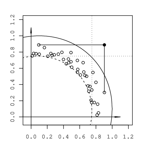
Proof For the sake of simplicity assume . Let denote the coordinatewise supremum of . Since is blunt there exists a such that the shifted quadrant and the set are disjoint (see Figure 1a). Let be the mean measure of . Then and both and go to infinity by Definition 5. The lemma above applied to the shifted clouds shows that the probability of a record in the sample cloud vanishes for . 
In order to complete the proof of Theorem 3.11, we now establish a link between the asymptotic shape of the scaled level sets of a light-tailed density and the shape of the limit set of the associated sample clouds.
Proposition 4.4.
Let denote i.i.d. random vectors from a density . Then the sequence of scaled sample clouds converges onto the closure of the set as if the scaling constants are chosen appropriately.
Proof The density is shape equivalent to ; see Proposition 3.4. The function also lies in , and by rapid variation and monotonicity of for any and eventually on and off . By the pointwise inequality (3.17) the functions satisfy the same inequalities eventually if we replace by . The measure with density satisfies , , for any open set which intersects by Lemma 3.5. Choose such that for . Then is the mean measure of the sample cloud , and from Proposition 4.1 the sample clouds converge onto since their mean measures do. 
5 Examples
This section illustrates the applicability of Theorems 3.10, 3.11 and 4.3 in determining whether a given distribution has asymptotically independent components. We also wish to see whether the conditions are sharp.
For any open bounded convex set in the plane whose closure contains the origin, the function is integrable and hence for suitable is a probability density. Along rays it is an exponential function. If is uniformly distributed on then it is simple to decide when the coordinates and are asymptotically independent, but asymptotic independence of the the coordinates of the vector with density is a different matter, even in the simple example where is the intersection of a disk of radius centered in and the open set above the diagonal. The light-tailed examples below are of a more general nature.
Example 1.
(Rotund-exponential densities) Let have a continuous homothetic density with convex shape and generating function . If has a boundary and varies rapidly, the coordinates are asymptotically independent, and the sample clouds, properly scaled, converge onto the closure of the set by Theorem 3.10 and Proposition 3.9. Now assume more: is rotund, i.e. the boundary is with positive definite curvature in every point. Also assume that the generating function is asymptotic to a von Mises function . Then is a so-called rotund-exponential density, see [3], Sections 9 and 10. If one zooms in onto a boundary point of so as to distinguish individual sample points, the sample clouds converge to a Gauss-exponential point process: vaguely on . The limit is a Poisson point process with intensity if one chooses the normalization appropriately. Weak convergence holds on all halfspaces . The restriction of to the upper halfspace is a probability density. The corresponding vector has independent components. This vector is the limit of the high risk scenarios , properly normalized, where is the vector conditioned to lie in the halfspace , and moves off to infinity in the sense that . These results remain valid under certain perturbations (if the density is multiplied by a flat function , see Section 11 in [3]). Such a perturbation does not affect the asymptotic behaviour of the exponent , but may affect the limit shape (take with and with , . If we choose then still is flat, but the shape of the level sets no longer converges). See Proposition 14.1 in [3]. So we see that under the extra conditions on the homothetic density there are three alternative asymptotic descriptions of large sample clouds from this density. Convergence onto the closure of the set describes the global behaviour of the sample clouds; weak convergence in the space to a Poisson point process whose mean measure is the exponent measure of an extreme value limit law (Gumbel with independent components); weak convergence to the Gauss-exponential Poisson point process on certain halfspaces describes the local behaviour in boundary points of .
Example 2.
(Skew-normal densities) A symmetric density satisfies . It may be transformed into an asymmetric density by multiplication with a positive continuous asymmetric function which satisfies . The skew-normal distributions introduced in [2] have a density which is the product of a centered Gaussian density with covariance and the function , where is the standard normal df and a non-zero linear functional. These densities are log-concave (since is positive) and hence have convex level sets.
htb
We claim that for a convex set with boundary. Write . The function is asymptotic to for and vanishes for . Let satisfy and . Then and
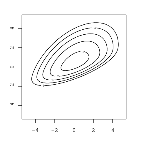
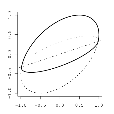
It follows from Proposition 3.9 that there is a limit shape: , which is the covariance ellipsoid on the halfspace where is positive, and a flattened version of this ellipsoid on the complementary halfspace, see Figure 2. The set is convex. To see that the boundary is , choose coordinates such that the underlying Gaussian density is standard, with spherical level sets, and then choose the vertical coordinate in the direction of . In these coordinates agrees with the unit ball on the upper halfspace, and with the cylinder symmetric ellipsoid for some on the lower halfspace . For boundary points in the horizontal coordinate plane the tangent plane is vertical: . Theorem 3.10 applies. If has a skew-normal distribution then the random variables are asymptotically independent whenever the linear functionals are linearly independent. Asymptotic independence of the skew-normal distribution has been partially proven in [18] using a direct analytic approach based on Sibuya’s condition.
Example 3.
Densities of the form for have level sets which are balls in . Lower dimensional marginals have the same form but with a different generator, since the projection of the -dimensional unit ball on the space spanned by the first coordinates is the -dimensional unit ball. The two-dimensional unit ball is blunt for all , and hence vectors with light-tailed densities as above have asymptotically independent coordinates. However for , the sup-norm, the unit ball is a cube , and the square is not blunt. The components of are still asymptotically independent, but we need extra work to prove this. The bivariate margins of have the same form with a different generator which still is continuous, strictly decreasing and rapidly varying in . (The cubic slices are replaced by square slices.) It suffices to consider bivariate densities for continuous, strictly decreasing positive functions on which vary rapidly in . The marginals of , , are equal by symmetry, and where by rapid variation of . Hence for , and by l’Hospital’s rule also the quotient . Thus Sibuya’s condition holds. However, asymptotic independence need not hold if the level sets are only asymptotically cubic, see Example 2 in [5].
Another example showing that results for do not need to carry over to is given in the Appendix, Example A.5. Our last example illustrates an asymptotically dependent distribution with a density in where bivariate projections of are non-blunt.
Example 4.
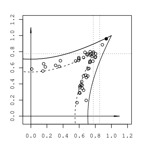
Let have a bivariate density with degrees of freedom. Transform the marginals to obtain a vector with standard Gaussian components. The new density is called a meta- density; see [20] p.193. It has normal marginals but the copula of the elliptic distribution. The shape of the level sets of the density converges to the symmetric subset of the square , see [4]. Figure 1b shows a detail. The set is not blunt, and the components of are asymptotically dependent since those of are.
6 Conclusion
We have explored conditions for asymptotic independence of the components of a multivariate random vector expressed in terms of the limiting shape of the level sets of the underlying density. A distinction had to be made between light and heavy tails. For light-tailed densities, the limiting shape of level sets is essential in determining whether asymptotic independence holds. In contrast, for heavy-tailed densities the (limiting) shape of level sets is irrelevant as long as the shape intersects the positive orthant. In the light-tailed case there is a simple sufficient condition for asymptotic independence of two components in terms of the corresponding bivariate projection of the shape. This subset of the plane has to be blunt. The more delicate question of the relation between shape and asymptotic independence when the bivariate projection is not blunt will be treated in a future publication.
Asymptotic dependence is a basic concern in multivariate risk analysis. The light-tailed densities studied in this paper have the property that sample clouds will have the same shape as the level sets of the density asymptotically. For sample clouds persistence of the shape, as the number of sample points increases, opens the possibility of using the shape to construct densities over the whole space. This makes it possible to estimate probabilities of regions far out which contain only a few or no sample points.
Acknowledgments
We are thankful to Paul Embrechts for drawing our attention to the problem considered in this paper and for several useful discussions.
Appendix A Appendix
A.1 Supplementary results
Proposition A.1.
Let be independent observations from the continuous df on . The probability of a record amongst the first observations goes to zero if and only if is asymptotically independent.
Proof We may assume that is a copula. Set . Then the Poisson approximation gives a probability to the event: among the first observations there is exactly one in the complement of , and that observation lies in the square .. In case of asymptotic dependence for some subsequence, and hence the probability of a record in a sample of size will exceed eventually. Conversely, asymptotic independence implies for any , whereas the marginals satisfy . As in Lemma 4.2 the probability of a record vanishes. 
Proposition A.2.
Suppose and the generator varies regularly or satisfies -variation
| (A.1) |
Then is shape equivalent to if and only if .
Proof Condition (A.1) implies that for every there exists such that for all . Let . Suppose . Then for any the point eventually lies in the ring on which fluctuates by a factor at most . To show the converse, suppose satisfies (A.1) and let so that for . Then for any eventually
and since is arbitrary, we have for as required for shape equivalence by (3.14). 
A.2 Counterexamples
This section contains counterexamples mentioned in the main text.
Example A.1.
A density may have spherical level sets without exhibiting spherical symmetry. This will be the case if is an off-center ball with for some . To be star-shaped the origin has to lie in , or be a boundary point. In the latter case the set is a ball (if is a bounded interval) or an open halfspace.
Example A.2.
For any there exists a bounded open star-shaped set which contains the origin, whose closure is the cube , and such that the volume of is small, . To construct such a star-shaped set take a dense sequence on the boundary , and define as the union of open disks with center and radius , where so fast that the area of is . Now let be the union of an open centered ball with volume and the set of all points with and .
Example A.3.
Consider a continuous strictly positive density on whose level sets all have the same shape. The set is convex, even rotund, and the function is continuous and strictly increasing. The marginal densities are not necessarily all unimodal.
Let be the uniform density on the tetrahedron with two vertices in the horizontal plane, say and . The other two vertices are and . Here is a positive integer to be chosen later. The marginal along the vertical axis along the base vector has a continuous density on which is parabolic on the interval and on , vanishing in the endpoints of the interval and with a maximum in the origin. The shifted tetrahedron contains the origin as interior point. Its vertical marginal density is shifted upwards over and has its maximum in . The vertical marginal density of the uniform distribution on the tetrahedron has its maximum in . The fair mixture of the uniform distribution on and has a density whose marginal is not convex if is large (since the left derivative of in is large). Now choose rotund sets converging to and densities converging to which satisfy the conditions of the example. If infinitely many of the vertical marginals were unimodal then the limit would be. We conclude that eventually is not unimodal.
Example A.4.
In view of Lemma 3.8 we see that is shape equivalent to for a continuous function precisely if for a function . Here are some examples of functions which are shape equivalent to the standard normal density on the plane, for a continuous positive function . One may take to be one of the following functions , with , , where . These functions may be multiplied with a function like which fluctuates rapidly but is weakly asymptotic to a constant. The level sets then will look locally like a shore with many small islands, and lakes, even though the sets are asymptotic to disks with .
Example A.5.
Let be the open triangle with vertices , and . It contains the origin. Let have convex level sets and be shape equivalent to . It is possible that is asymptotically independent. Suppose the function has triangular level sets . Let have level sets . Then agrees with the triangle except that the extreme top has been sliced off. If we choose , then
where for the halfspace . Let have density and let have density . Then weakly on . Since is finite and gives infinite weight to the halfspaces and , Sibuya’s condition holds by Proposition 2.3 with curve , .
References
- [1] B.C. Arnold, E. Castillo, and J.M. Sarabia. Multivariate distributions defined in terms of contours. J. Statist. Plann. Inference, 138:4158–4171, 2008.
- [2] A. Azzalini and A. Dalla Valle. The multivariate skew-normal distribution. Biometrika, 83:715–726, 1996.
- [3] G. Balkema and P. Embrechts. High Risk Scenarios and Extremes. A Geometric Approach. European Mathematical Society, Zurich, 2007.
- [4] G. Balkema, P. Embrechts, and N. Nolde. Meta densities and the shape of their sample clouds. Submitted, 2009.
- [5] G. Balkema, P. Embrechts, and N. Nolde. Sensitivity of the limit shape of sample clouds from meta densities. Preprint, 2009.
- [6] N.H. Bingham, C.M. Goldie, and J.L. Teugels. Regular Variation. Cambridge University Press, Cambridge, 1987.
- [7] K.W. Breitung. Asymptotic approximations for probability integrals. Lecture Notes in Mathematics. Springer-Verlag, 1994.
- [8] L. de Haan and A. Ferreira. Extreme Value Theory. An Introduction. Springer-Verlag, 2006.
- [9] S.W. Dharmadhikari and K. Joag-Dev. Unimodality, Convexity, and Applications. Academic Press, Inc., San Diego, 1988.
- [10] K.-T. Fang, S. Kotz, and K.-W. Ng. Symmetric multivariate and related distributions. Chapman and Hall, 1990.
- [11] C. Fernandez, J. Osiewalski, and M.F.J. Steel. Modeling and inference with v-spherical distributions. J. Amer. Statist. Assoc., 90(432):1331–1340, 1995.
- [12] A.V. Gnedin. On multivariate extremal processes. J. Multivariate Anal., 46:207–213, 1993.
- [13] A.V. Gnedin. On the best choice problem with dependent criteria. J. Appl. Probab., 31:221–234, 1994.
- [14] E. Hashorva. Extremes of asymptotically spherical and elliptical random vectors. Insur.: Math. Econ., 36:285–302, 2005.
- [15] H. Hult and F. Lindskog. Multivariate extremes, aggregation and dependence in elliptical distributions. Adv. Appl. Prob., 34:587–608, 2002.
- [16] K. Kinoshita and S.I. Resnick. Convergence of scaled random samples in . Ann. Probab., 19:1640–1663, 1991.
- [17] A. Ledford and J. Tawn. Statistics for near independence in multivariate extreme values. Biometrika, 83(1):169–187, 1996.
- [18] N. Lysenko, P. Roy, and R. Waeber. Multivariate extremes of generalized skew-normal distributions. Statist. Probab. Let., 79:525–533, 2009.
- [19] K. Maulik, S.I. Resnick, and H. Rootzén. Asymptotic independence and a network traffic model. J. Appl. Prob., 39:671–699, 2002.
- [20] A. J. McNeil, R. Frey, and P. Embrechts. Quantitative Risk Management: Concepts, Techniques and Tools. Princeton University Press, Princeton, 2005.
- [21] T. Mikosch. Copulas: Tales and facts. Extremes, 9:3–20, 2006.
- [22] J. Osiewalski and M.F.J. Steel. Robust bayesian inference in -spherical models. Biometrika, 80:456–460, 1993.
- [23] A. Ramos and A. Ledford. A new class of models for bivariate joint tails. J. Roy. Statist. Soc. B, 71(1):219–241, 2009.
- [24] S.I. Resnick. Extreme Values, Regular Variation, and Point Processes. Springer, 1987.
- [25] S.I. Resnick. Hidden regular variation, second order regular valuation and asymptotic independence. Extremes, 5:303–336, 2002.
- [26] M. Sibuya. Bivariate extreme statistics. Ann. Inst. Stat. Math., 11:195–210, 1960.