A Quantum Monte Carlo Method at Fixed Energy

Quantum Monte Carlo methods are widely used to compute properties of quantum systems using classical sampling algorithms. In this paper we develop a novel Quantum Monte Carlo method that allows one to numerically investigate ground state properties of a quantum system.

A virtue of Quantum Monte Carlo is that one is not required to manipulate vectors in the Hilbert space corresponding to the quantum system. The dimension of this Hilbert space typically grows exponentially with the physical size of the system. Instead, Quantum Monte Carlo methods map the problem of approximating the ground state energy (or some other observable) onto the problem of evaluating an expectation value with respect to a probability distribution $q(X)$ over a set of configurations $C$ (so $X\in C$). In order to evaluate this expectation value, one can use a classical Markov chain Monte Carlo algorithm to sample configurations from the distribution $q$. Markov chain Monte Carlo works by defining a Markov chain on the space of configurations $C$. This Markov chain can be described by an update rule which tells you how to generate a new configuration of the chain from the current one. The Markov chain is constructed so that the limiting distribution is $q(X)$. One then applies some large number $N_{0}$ of iterations of the Markov chain to some initial configuration $X_{0}$. If $N_{0}$ is sufficiently large then after these iterations, the distribution of subsequent configurations will be arbitrarily close to $q$.

We now give a brief description of how our method is used to estimate properties of the ground state. We write the Hamiltonian as $H(\lambda)=H_{0}+\lambda V$, where $H_{0}$ is diagonal in a given basis $\{|z\rangle\}$ and $\lambda V$ is off diagonal in this basis. (In an n spin system $z$ is an n bit string.) In section II we outline our assumptions and restrictions on $H_{0}$ and $V$. With these choices, the ground state energy is always less than or equal to zero, and we will see that for each value of $E<0,$ there exists one positive value $\lambda(E)$ such that the ground state of $H(\lambda(E))$ has energy E. To use our Monte Carlo method, one first must fix $E<0$ and a large integer $m$. We define a path of length $m$ to be a sequence $\{z_{1},...,z_{m}\}$, where each $n$ bit string $z_{i}$ is the label of the state $|z_{i}\rangle$. These paths are the configurations of the previous paragraph. We will define a probability distribution $f(\{z_{1},...,z_{m}\})$ over the set of all paths of length m (this distribution is also a function of the value of $E$ which was chosen). We will show how the function $\lambda(E)$ can be obtained by computing an average with respect to the probability distribution $f$.

To motivate our method and to get a general idea of how it works, consider the function

Assuming that $E<0$ and $\lambda>0$ are chosen so that the Taylor series expansion converges, we can write

It is clear from the expression in equation 1 that the function $G(E,\lambda)$ blows up when $E\rightarrow E_{g}(\lambda)$, where $E_{g}(\lambda)$ is the ground state energy of $H(\lambda)$. Equivalently we can say that at a fixed value of $E$ the blow up occurs as $\lambda\rightarrow\lambda(E)$, where $E_{g}(\lambda(E))=E.$ At this value of $\lambda$ the Taylor series expansion must diverge. In fact, this divergence occurs because as $m$ becomes large, terms in the series approach 1 for large $m$ (here we have made some assumptions about the Hamiltonian which we discuss in the next section) so

For the remainder of this section we assume that $m$ is large enough to make $\approx$ close to $=$. By inserting complete sets of states in the basis that diagonalizes $H_{0}$ we can express the LHS as a sum over paths

where $E_{i}=\langle z_{i}|H_{0}|z_{i}\rangle$. Now taking the log and differentiating with respect to $E$, we obtain

Here the expectation value is taken with respect to the measure $f$ on paths defined by

where $F$ is a normalizing constant. We will show how to sample with respect to the distribution $f$ in a way that makes numerical work possible. Sampling from the distribution $f$ will also allow us to compute $-\frac{1}{\lambda(E)}\frac{d\lambda(E)}{dE}$ from equation 3 as well as other properties of the ground state.

Our paper is organized as follows. In section II we describe the types of Hamiltonians for which our method applies. In section III we outline the new method that we propose. In section IV we explicitly construct Monte Carlo update rules for the case where $V=-\sum_{i=1}^{n}\sigma_{x}^{i}$, and we give numerical data using our algorithm at $n=16$ where we are able to compare with exact diagonalization. In section V we review the continuous imaginary time Quantum Monte Carlo method [6], which is based on the thermal path integral. We also derive a novel estimator in this ensemble of paths for the ground state energy which becomes exact in the limit $\beta\rightarrow\infty.$

We consider finite dimensional Hamiltonians of the form

where $H_{0}$ is diagonal in a given basis $\{|z\rangle\}$, and $V$ has zeros along the diagonal in this basis. We make the following assumptions about the Hamiltonian:

1. 1.

   The off diagonal matrix elements of $V$ in the basis $\{|z\rangle\}$ which diagonalizes $H_{0}$ are all either negative or zero. (This ensures that our Quantum Monte Carlo method will not suffer from a sign problem.)

2. 2.

   The ground state of $H(\lambda)$ is not degenerate for any value of $\lambda\in(-\infty,\infty).$

3. 3.

   The smallest eigenvalue of $H_{0}$ is zero. Note that this condition can be fulfilled without loss of generality by adding a constant term to the Hamiltonian. Writing $|z_{0}\rangle\in\{|z\rangle\}$ for the unique state with $H_{0}|z_{0}\rangle=0$, we further require that $V|z_{0}\rangle\neq 0$ . (This implies that $|z_{0}\rangle$ is not an eigenvector of $V$ since $\langle z_{0}|V|z_{0}\rangle=0$ follows from assumption 1 above.)

We write $|\psi_{g}(\lambda)\rangle$ and $E_{g}(\lambda)$ for the ground state eigenvector and ground state energy of $H(\lambda)$ . From second order perturbation theory in $\lambda$, we have that

where the inequality is strict because $V|z_{0}\rangle\neq 0$.

Using the fact that

we show that

In order to obtain the inequalities, we use the variational principle. When $\lambda>0,$ the ground state energy must be less than zero, since $|z_{0}\rangle$ has zero expectation value for $H$ (and $|z_{0}\rangle$ is not an eigenvector of $H(\lambda)$). This, together with the fact that $H_{0}$ is positive semidefinite, implies that $\langle\psi_{g}|V|\psi_{g}\rangle<0.$ The analogous result for $\lambda<0$ is obtained in the same way. These inequalities give a qualitative picture of the curve $E_{g}(\lambda)$. Starting from $E_{g}(0)=0,$ the curve slopes downwards as it goes out from $\lambda$=0, and approaches $-\infty$ on both sides of the origin for sufficiently large $|\lambda|.$ Note that this implies that for each $E<0$ there is one positive and one negative value of $\lambda$ (call them $\lambda(E)$ and $\lambda_{-}(E)$ respectively) such that $E_{g}(\lambda(E))=E$ and $E_{g}(\lambda_{-}(E))=E$. Furthermore, we show in appendix A.1 that it is always the case that

We refer to the case where the inequality is strict as the generic case. We illustrate the qualitative features of the curve $E_{g}(\lambda)$ (for the generic case) in figure 1.

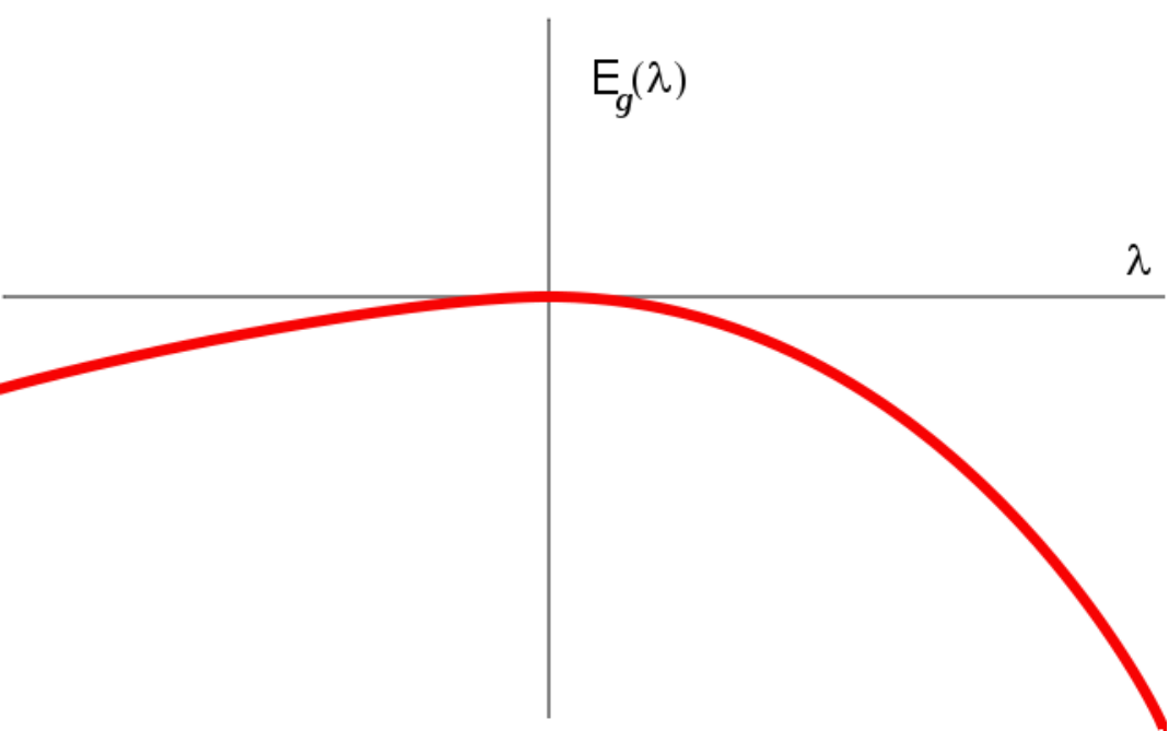
In the nongeneric case where equality holds at some particular value of $E$ , then in fact equality holds at every value of $E$ and the curve $E_{g}(\lambda)$ is symmetric about $\lambda=0$.

We now explicitly construct a method to compute averages with respect to the distribution $f$ in the case where the Hilbert space is that of n spin $\frac{1}{2}$ particles, and $V=-\sum_{i=1}^{n}\sigma_{x}^{i}$. The Hamiltonian $H_{0}$ is an arbitrary diagonal matrix in the Pauli z basis for $n$ spins. Our algorithm can be used to compute the average of any function of the path which is invariant under cyclic permutations of the path. For this choice of $V$, the spectrum of $H(\lambda)$ is symmetric about $\lambda=0$ (so this corresponds to the nongeneric case where equality holds in equation 6 for all $E<0$). With these choices, the paths which have nonzero weight (with respect to $f$) are periodic paths of $m$ bit strings of length $n$ where each string $z$ differs from the previous one by a bit flip. We must take $m$ to be even since each bit must flip an even number of times so that the path is periodic (and so the total number of bit flips $m$ in the path must be even). In order to sample from these paths according to $f$, we construct a Markov Chain which has $f$ as its limiting distribution (actually, our Markov Chain converges to the correct distribution over equivalence classes of paths which are only defined up to cyclic permutation–this is why we restrict ourselves to estimating quantities which are cyclically invariant). Note that with our choice of $V$ we can write (see equation 7)

Our Markov chain is defined by the following update rule which describes how the configuration is changed at each step

1. 1.

   Choose an integer $i\in\{1,...,m\}$ uniformly at random.

2. 2.

   Consider the bit strings $z_{i-1},z_{i},z_{i+1}$ in the current path (where $z_{m+1}=z_{1}$). Suppose that $z_{i-1}$ and $z_{i}$ differ in bit $q_{1}\in\{1,...,n\}$, which we write as $z_{i}=z_{i-1}\oplus\hat{e}_{q_{1}}$. Also write $q_{2}\in\{1,...,n\}$ for the bit in which $z_{i}$ and $z_{i+1}$ differ, so $z_{i+1}=z_{i}\oplus\hat{e}_{q_{2}}$.

3. 3.

   If $q_{1}\neq q_{2}$ then propose to change the bit string $z_{i}$ to the new value $\tilde{z}_{i}=z_{i-1}\oplus\hat{e}_{q_{2}}.$ Accept this proposal with probability

   $$P_{accept}=\min\left\{1,\frac{E_{i}-E}{\tilde{E}_{i}-E}\right\}$$

   where $\tilde{E}_{i}=\langle\tilde{z}_{i}|H_{0}|\tilde{z}_{i}\rangle$. This Monte Carlo move has the effect of interchanging 2 consecutive flips in the path (see figure 2).

4. 4.

   If $q_{1}=q_{2}$ , then choose a new bit $q_{new}\in\{1,...,n\}$ from the probability distribution

   $$P(q_{new}=q)=\frac{1}{W}\frac{1}{E_{q}^{\prime}-E}$$

   (16)

   where $E_{q}^{\prime}=\langle z_{i-1}\oplus\hat{e}_{q}|H_{0}|z_{i-1}\oplus\hat{e}_{q}\rangle$, and $W=\sum_{j=1}^{n}\frac{1}{E_{j}^{\prime}-E}$. Then (with probability 1) change $z_{i}$ to the new value $z_{i-1}\oplus\hat{e}_{q_{new}}$. This Monte Carlo move replaces a pair of consecutive flips which occur in the same bit with 2 new flips in a possibly different bit (see figure 3).

We show in appendix C that this algorithm can be used to estimate any quantity which is invariant under cyclic permutations of the path (note that all estimators we have discussed have this property).

In the ensemble of paths which was considered in the previous section, the parameters $m$ and $E$ are fixed and then quantities $\bar{\beta}(E,m)$ and $\overline{\lambda^{2}}(E,m)$ are computed as ensemble averages. In this section we review the standard approach to computing thermal averages using continuous imaginary time Quantum Monte Carlo [6]. To use this method, parameters $\beta$ and $\lambda$ are fixed beforehand and quantities $\bar{E}(\beta,\lambda)$ and $\bar{m}(\beta,\lambda)$ are computed as ensemble averages. We will also derive a new estimator for $\langle H\rangle=\frac{Tr[He^{-\beta H}]}{Z(\beta)}$ which is valid for large $\beta$ simulations. The form of this estimator establishes a connection between the continuous imaginary time Quantum Monte Carlo method and the new method that we outlined in the previous section.

The standard method [6] is based on the expansion of the partition function

where $V_{I}(t)=e^{tH_{0}}Ve^{-tH_{0}}$ and $E_{i}=\langle z_{i}|H_{0}|z_{i}\rangle$. This expression is interpreted as a path integral, where a path is defined by a piecewise constant function $z(t)$ for $t\in[0,\beta]$. The function $z(t)$ takes values in the set $\{z\}$ which are the labels of the basis states $\{|z\rangle\}$ which diagonalize $H_{0}.$ In the above expression for $Z(\beta)$, we have

The allowed values of $m$ are $2,3,4,5,...$ as well as $m=0$ in which case the path is constant $z(t)=z_{1}$ (for some $z_{1}$) for all $t\in[0,\beta]$.

We define $H_{0}(z(t))$ to be $\langle z(t)|H_{0}|z(t)\rangle$, so $\int_{0}^{\beta}H_{0}(z(t))dt=E_{1}t_{1}+E_{2}(t_{2}-t_{1})+...+E_{1}(\beta-t_{m})$ . Equation 17 can be used to define a measure $\rho$ on paths in imaginary time. The probability of a given path parameterized by $z(t)$ is

where $Z(\beta)$ is the normalization. Our assumption that off diagonal elements of $V$ are nonpositive guarantees that $\rho\geq 0$. The task of sampling paths from the distribution $\rho$ can be accomplished using Markov chain Monte Carlo methods such as those outlined in references [4, 6, 2]. By using these methods to sample paths from this probability distribution, one can compute physical properties of the quantum system at an inverse temperature $\beta.$ Known estimators for the expectation of the terms in the Hamiltonian are (see appendix B)

Here $m$ is the number of transitions in the path $z(t)$ and is not fixed. Note that the estimator for $\langle\lambda V\rangle$ only involves the number of transitions in the path. The above two estimators can be combined to obtain $\langle H\rangle$. One can also obtain the following expressions for the variances of these estimators in the limit $\beta\rightarrow\infty$

This shows that as $\beta\rightarrow\infty$, the distributions for these estimators become sharply peaked about their mean values. We define intensive ensemble averages

which in the $\beta\to\infty$ limit become respectively the ground state expectation value of $-\lambda V$ and the ground state energy.

We have outlined a new approach to Quantum Monte Carlo simulations in which properties of the ground state of a quantum system are computed at a fixed value of the ground state energy. We have confirmed the validity of our method by performing a numerical simulation of a system consisting of 16 spins. Our approach involves a path integral which does not include any jump time variables, as in the stochastic series expansion [7, 8]. We have also obtained a new estimator for the ground state energy which is valid in continuous imaginary time Quantum Monte Carlo simulations but which does not involve the imaginary time variables. We hope that our method will be applied to numerical simulations that go beyond the toy system studied in this paper.

The authors thank Sam Gutmann for useful discussions. This work was supported in part by funds provided by the U.S. Department of Energy under cooperative research agreement DE-FG02-94ER40818, the W. M. Keck Foundation Center for Extreme Quantum Information Theory, the U.S Army Research Laboratory’s Army Research Office through grant number W911NF-09-1-0438, the National Science Foundation through grant number CCF-0829421, and the Natural Sciences and Engineering Research Council of Canada.

References

- [1] B.B. Beard. Extending monte carlo samples. Nuclear Physics B - Proceedings Supplements, 119:1012 – 1014, 2003. Proceedings of the XXth International Symposium on Lattice Field Theory.
- [2] Edward Farhi, Jeffrey Goldstone, David Gosset, Sam Gutmann, Harvey B. Meyer, and Peter Shor. Quantum adiabatic algorithms, small gaps, and different paths, 2009. arXiv:0909.4766.
- [3] Edward Farhi, Jeffrey Goldstone, Sam Gutmann, Joshua Lapan, Andrew Lundgren, and Daniel Preda. A quantum adiabatic evolution algorithm applied to random instances of an NP-complete problem. Science, 292:472–475, 2001. arXiv:quant-ph/0104129.
- [4] Florent Krzakala, Alberto Rosso, Guilhem Semerjian, and Francesco Zamponi. On the path integral representation for quantum spin models and its application to the quantum cavity method and to monte carlo simulations. Physical Review B, 78:134428, 2008.
- [5] M. Newman and G. Barkema. Monte Carlo Methods in Statistical Physics. Clarendon Press, 1999.
- [6] N. V. Prokof’ev, B. V. Svistunov, and I. S. Tupitsyn. Exact quantum monte carlo process for the statistics of discrete systems. ZH.EKS.TEOR.FIZ., 64:853, 1996.
- [7] A W Sandvik. A generalization of handscomb’s quantum monte carlo scheme-application to the 1d hubbard model. Journal of Physics A: Mathematical and General, 25(13):3667–3682, 1992.
- [8] A. W. Sandvik, R. R. P. Singh, and D. K. Campbell. Quantum monte carlo in the interaction representation — application to a spin-peierls model. Physical Review B, 56:14510, 1997.
- [9] Masuo Suzuki. Relationship between -dimensional quantal spin systems and -dimensional ising systems. Progress of Theoretical Physics, 56(5):1454–1469, 1976.
- [10] Ulli Wolff. Monte carlo errors with less errors. Comput.Phys.Commun.156:143-153,2004; Erratum-ibid.176:383,2007.
Appendix A Derivation of Estimators For the New Monte Carlo Method
A.1 Properties of the operator
Our analysis of the new Monte Carlo method is based on properties of the operator
as was seen from the Introduction.
We take and is defined to be the positive value of such that the ground state of has energy . We will show the following properties of this operator:
- 1.
All eigenvalues of are real and in absolute value.
- 2.
is an eigenvector of with eigenvalue It may also be the case that is an eigenvector of with eigenvalue There are no other eigenvectors of with eigenvalues .
The second property says that the subspace of states spanned by eigenvectors of with eigenvalues is either 1 or 2 dimensional. We will see that the case where it is two dimensional occurs only when has ground state energy .
To show that eigenvalues of are real whenever , note that the spectrum of is the same as the spectrum of the operator
which is Hermitian.
Now suppose (to reach a contradiction) that is an eigenvector of with eigenvalue Then
which says that there exists an eigenvector of with eigenvalue . In section II we proved that the ground state energy of is strictly decreasing for positive , which means that no eigenvector of can have energy smaller than or equal to . This is a contradiction and so all positive eigenvalues of are
Now, since we have proven that all eigenvalues of are , if it is the case that some negative eigenvalue of is then the eigenvalue of which is largest in magnitude has negative sign. If this were true, then the limit
would be equal to a negative constant. But this cannot be the case since all matrix elements of are positive or zero. So we have shown property 1.
We now proceed to show property 2 which was stated earlier in the appendix, and in the process we prove the inequality 6 from section II. The real nonzero eigenvalues of can be related to eigenvalues of for some value of . In particular, suppose that is a real nonzero eigenvalue of with eigenvector . Then
so
Let us write the eigenvalues of as
(which follows by property 1.) Then the values of at which has an eigenvalue with energy are
for . Write for the negative value of lambda such that has ground state energy . The values of which are smallest in magnitude (and hence closest to the axis ) are and and these correspond to the ground state at energy , with . All other values are greater than in magnitude. This proves inequality 6, and also shows property 2 described above.
A.2 Derivation of the Estimators and
Having derived properties 1. and 2. of the operator in the previous section, we now proceed to use these properties to prove equations 14 and 15.
Our treatment below applies to both the generic case where inequality 6 is strict as well as the nongeneric case where equality holds as long as in the latter case is always even. In either case we have