A Compact Microchip-Based Atomic Clock Based on Ultracold Trapped Rb Atoms

Consider the three-level system shown in Fig. 1 in the presence of an electromagnetic field given by

The field consists of two components: a probe beam of amplitude $\bm{A}_{31}$ and frequency $\omega_{31}$ that is nearly resonant with the transition $|1\rangle\rightarrow|3\rangle$, and a coupling beam of amplitude $\bm{A}_{32}$ and frequency $\omega_{32}$ that is nearly resonant with the transition $|2\rangle\rightarrow|3\rangle$. Light changes the optical properties of the medium because it affects the evolution of the atomic density operator $\rho$. The evolution equation for $\rho$ is

where $H_{a}$ is the atomic Hamiltonian in the absence of light and $H_{int}=-\bm{D}\cdot{\bm{\mathcal{E}}}(t)$ is the dipole interaction Hamiltonian between the light field and the atom. $\bm{D}$ is the dipole moment operator and $R_{\rho}$ is the relaxation operator.

An electric dipole transition between clock states $|1\rangle$ and $|2\rangle$ is not allowed by selection rules. The resulting atomic dipole operator has the form

where $\bm{\mu}_{mn}=\langle m|{\bm{D}}|n\rangle$ is the dipole transition matrix element. The Hamiltonian $H=H_{a}+H_{int}$ in the rotating-frame approximation can be written

where $\Omega_{31}=\bm{\mu}_{31}\cdot\bm{A}_{31}/\hbar$ and $\Omega_{32}=\bm{\mu}_{32}\cdot\bm{A}_{32}/\hbar$ are the Rabi frequencies of the probe and coupling transitions, respectively.

Evolution of the electromagnetic field is governed by Maxwell’s equations, which reduce to

where $\bm{\mathcal{P}}$ is the polarization of the medium. The atomic dipole operator is given by Eqn. 4, so the single atom polarization is

The polarization $\bm{\mathcal{P}}$ of the medium is given by the relation

where $n_{a}$ is the density of atoms. The steady-state response of the term ${\bm{P}}_{31}$ oscillates at the frequency $\omega_{31}$ $({\bm{P}}_{31}\propto\exp(-\omega_{31}t))$ and the term ${\bm{P}}_{32}$ oscillates at the frequency $\omega_{32}$.

Eqns. 3 and 5 show that the coherences, or off-diagon-al elements of the density matrix, can be written as $\rho_{31}=\sigma_{31}\exp(-i\omega_{31}t)$ and $\rho_{32}=\sigma_{32}\exp(-i\omega_{32}t)$, where the functions $\sigma_{ij}$ are slow functions of time as compared with the exponentials. It is convenient to factor out the fast time dependence from the problem and work with slow-varying elements of the density matrix. This is achieved by going to the interaction representation, i.e. factorizing the Hamiltonian in Eqn. 5 as $H=H_{0}+V$ and introducing the interaction-representation density operator $\sigma$ by the relation $\sigma=\exp(iH_{0}t/\hbar)\rho\exp(-iH_{0}t/\hbar)$. The density operator $\sigma$ obeys the equation

where

is the interaction Hamiltonian. Similarly, $R_{\sigma}$ is the relaxation operator in the interaction representation.

The Hamiltonian $H_{0}$ should be chosen so that elements of the density matrix $\sigma$ are slow functions of time, i.e. do not contain fast time scales on the order of inverses of laser frequencies. A convenient choice is

and

where $\Delta_{31}=\omega_{31}-(\omega_{3}-\omega_{1})$ and $\Delta_{32}=\omega_{32}-(\omega_{3}-\omega_{2})$ are the detunings of the two lasers from the frequencies of the corresponding transitions with which they are nearly resonant.

The slowly-varying density matrix $\sigma$ is related to the full density matrix $\rho$ by

The interaction Hamiltonian $V_{I}$ in Eqn. 11 is given by the expression

The relaxation matrix is given by

The relaxation matrix includes the total spontaneous decay rate $\Gamma$ of the excited state; partial decay rates $\Gamma_{31}$ and $\Gamma_{32}$ of the excited state to the clock states $|1\rangle$ and $|2\rangle$, respectively; optical decoherences $\gamma_{c1}$ and $\gamma_{c2}$; and the Raman decoherence $\gamma_{c}$. The system is assumed to be open, implying that atoms are lost upon spontaneously decaying to states other than $|1\rangle$ or $|2\rangle$. As a result, the total decay rate of the excited state $\Gamma=(2\pi)6.0$ MHz is larger than the sum of the partial decay rates (see Table 1). We ignore decoherence between the clock states (i.e. $\gamma_{c}=0$) and set the optical decoherences equal to half of their corresponding partial decay rates (i.e. $\gamma_{c1}=\Gamma_{31}/2$ and $\gamma_{c2}=\Gamma_{32}/2$).

The set of equations for the elements of the density matrix takes the form

where the Raman detuning $\delta=\Delta_{31}-\Delta_{32}=(\omega_{31}-\omega_{32})-(\omega_{2}-\omega_{1})$ is the difference between laser difference frequency and the atomic clock frequency $\omega_{21}=\omega_{2}-\omega_{1}$. The common-mode detuning $\Delta_{0}=(\Delta_{31}+\Delta_{32})/2$ is the average of the two laser detunings.

The polarization of the atomic sample is given by

The relative dielectric constant of the medium is $\epsilon=1+\chi$, where $\chi$ is the medium susceptibility. Using Eqns. 6 and 18, $\chi$ becomes

where $\omega_{p}$ and $\omega_{c}$ are the probe and coupling optical frequencies, respectively.

Eqns. 17 were solved numerically using properties for the relevant transitions in ⁸⁷Rb (see Table 1). Both probe and coupling lasers are on resonance with their respective transitions (i.e. $\delta=0$ and $\Delta_{0}=0$). Several factors must be considered when choosing appropriate values for the Rabi frequencies. A longer response time, as needed for a smaller Rabi frequencies, permits the electronic signal processing to operate at lower bandwidths, which simplifies the detection circuitry. On the other hand, smaller Rabi frequencies result in lower optical powers that in turn leads to lower detection signal-to-noise ratios. Taking these considerations into account, we chose $\Omega_{c}=\Omega_{p}=(2\pi)150$ kHz for numerical estimates. Assuming a beam waist of 25 $\mu$m, the corresponding probe power is 130 pW.

Fig. 4 illustrates how the probe and coupling beams modify the density matrix populations. We assume the atomic sample starts entirely in state $|1\rangle$ (i.e. $\rho_{11}=1$, $\rho_{22}=\rho_{33}=0$), although any choice of initial conditions will lead to the same steady-state response of equal clock state populations ($\rho_{11}=\rho_{22}$). The steady-state population $\rho_{33}=0$ in the presence of resonant laser fields is the clearest indication that the sample becomes optically transparent. Note that the excited state population $\rho_{33}$ briefly becomes non-zero. Although a large fraction of this excited state population decays into the dark coherent state, the remainder decays to ground state sublevels other than the clock states. Atoms in these other ground states will no longer be trapped and can therefore escape from the atomic cloud. The result is steady-state populations that sum to less than 1. Assuming these untrapped atoms are initially at rest, either gravity or a magnetic force will force them to fall out of the trap in less than 5 ms (ignoring collisions with other atoms). Although these untrapped atoms remain in the atomic cloud for the entire duration of the first pulse, they are not resonant with probe and coupling beams due to the magnetic field that lifts the degeneracy of magnetic sublevels.

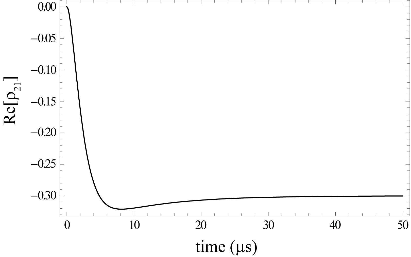
Fig. 5 shows how coherence between the clock states is created during the initial pulse. For an equal superposition state, the coherence between clock states, given by the off-diagonal element $\rho_{21}$ of the density matrix, attains a final value $\rho^{(1)}_{21}$ equal in magnitude to the clock state populations $\rho_{11}$ and $\rho_{22}$. It is this non-zero coherence that differentiates atoms in a superposition state from atoms in equal populations of two different atomic eigenstates.

After the initial EIT pulse, atoms precess in the dark for time $T$, during which the coherence $\rho^{(1)}_{21}$ picks up a phase shift factor $\mathrm{exp}(-\delta\,T)$. After precession, the second EIT pulse is applied. We assume that values of the Rabi frequencies $\Omega_{c}$ and $\Omega_{p}$, Raman detuning $\delta$, and common-mode detuning $\Delta_{0}$ are equal to those used for the first pulse. Eqns. 17 are again solved numerically, this time using $\rho^{(1)}_{21}\mathrm{exp}(-\delta\,T)$ for the initial value of the coherence. The clock state populations obtained at the end of the first pulse are used as the initial values for the second pulse.

The optical phase shift is given by $\Delta\phi=2\pi l(n^{\prime}-1)/\lambda$, where $l$ is the length of the atomic sample in the propagation direction of the probe laser and the real component of the refractive index is given by $n^{\prime}=\mathrm{Re}[\sqrt{1+\chi(\omega_{p})}]$. Fig. 6 illustrates the calculated optical phase shift as a function of time. When the laser difference frequency is resonant with the clock frequency $\omega_{21}$ (i.e. $\delta=0$), the sample is transparent and there is no phase shift (red). The maximum phase shift (black) occurs for $\delta=\pm 2\pi\times 1/(4T)$ Hz.

The detected photocurrent is given by $I=2\mathcal{R}\sqrt{P_{w}P_{s}}\phi$, where $\mathcal{R}$ is the responsivity of the photodetector. To maximize signal-to-noise, the photocurrent is numerically integrated up to time $t_{2}$. Ramsey fringes of FWHM $\Gamma_{R}=1/(2T)$ are visible in Fig. 7, which shows the integrated photocurrent as a function of Raman detuning $\delta$. Unlike fringes that are obtained from absorption measurements, fringes obtained from optical phase shifts are dispersive and therefore have a zero-crossing at $\delta=0$. As a result, for small $\delta$, the integrated photocurrent is directly proportional to the correction that must be applied to the laser difference frequency.

The expected noise is obtained by integrating the noise current $i_{n}$ over the duration $t_{2}$ of the second EIT pulse. This yields a noise charge $q_{n}$. Assuming the photodetection noise is determined by the photon shot noise of the strong probe laser, the rms noise current $\sigma_{i}$ is given by

where $e$ is the electron charge and the circuit bandwidth $2\pi\Delta f=1/\tau_{R}$ is the inverse of the characteristic response time $\tau_{R}$ of the circuit. The noise charge $q_{n}$ exhibits a random walk of duration $t_{2}$, yielding a mean-square noise charge $\langle q_{n}^{2}\rangle$ of

where $D=\sigma_{i}\,\tau_{R}$ is the diffusion coefficient. Eqn. 21 assumes that the circuit response time $\tau_{R}$ is much faster than $t_{2}$ (i.e. $\tau_{R}\ll t_{2}$). The rms noise charge $\sigma_{q}$ can then be expressed

Note that in the limit $\tau_{R}\ll t_{2}$, $\sigma_{q}$ depends only on $t_{2}$ and not on the circuit bandwidth.

The signal is obtained from the slope $S$ of the Ramsey fringe near $\delta=0$. The signal-to-noise ratio SNR=$S$/$\sigma_{q}$ is numerically calculated to be $\sim$7.5$\times 10^{4}$ for the experimental parameters listed in Table 2. The fractional frequency instability, as limited by noise of the optical detection, is

where $f_{0}=\omega_{21}/(2\pi)=6.8$ GHz is the clock frequency and $\tau$ is the integration time. The SNR of the optical detection is almost two orders of magnitude larger than the SNR due to atom shot noise alone (SNR$\,\sim\sqrt{N_{a}}=10^{3}$ for $N_{a}=10^{6}$ atoms):

Aside from systematic effects and technical noise sources, clock performance will therefore be limited by the atom shot noise.

AC Stark shifts, or light shifts, are one of the most problematic sources of systematic error in both miniature and full-size atomic clocks. The term “light shifts” refer to any effect that modifies the clock frequency through the atomic interaction with the laser fields (and other oscillating electromagnetic fields). The result is a clock whose accuracy ultimately depends on external experimental parameters instead of the inherent properties of the atomic species. In addition to accuracy, drift in these parameters can affect clock stability.

The advantage of pulsed EIT as a clock interrogation scheme is that a proper choice of Rabi frequencies (as determined by the laser intensities), EIT pulse duration, and common-mode laser detuning leads to a clock that is free of all light shifts. Our goal in this section is not to provide an accurate calculation that includes all sources of light shifts, which would be a computationally intensive task. Rather, we show that the shift-free configuration can be obtained for realistic operating parameters by just accounting for the the largest source of non-resonant light shifts. However, since the identification of shift-free parameters is best done experimentally, our numerically studies strongly suggest that an experimental approach would succeed in achieving a shift-free clock.

Light shifts can be divided into two categories. The first are shifts that arise from the resonant interaction of the two laser fields with the three-level atomic system (i.e. the idealized system represented in Fig. 1). These shifts, which we label “resonant”, have been studied experimentally in atomic beams and have been found to arise when the initial EIT laser pulse is extinguished before the steady-state response has been reached. For the case of a closed atomic system with excited state decay rate $\Gamma$, the resonant light shift $\Delta\delta$ can be expressed mathematically as

where $D_{0}$ is the difference in the initial clock state populations [23]. The Raman damping rate $\alpha$ and Raman dispersion $\beta$ are given by

where $\Omega$ is the Rabi frequency of both probe and coupling transitions (i.e. $\Omega_{p}=\Omega_{c}$) and the interrogation time $T$ is assumed to be much longer than the pulse duration $t_{1}$. The assumption of small common-mode detunings ($\Delta_{0}\ll\Gamma$) yields $\alpha\approx\Omega^{2}/(2\Gamma)$ and $\beta\approx\Omega^{2}\Delta_{0}/\Gamma^{2}$. The additional assumption that the argument of the arctangent is much less than 1 allows us to simplify Eqn. 25 to

Eqn. 28 shows how the resonant shift depends on various experimental parameters. The shifts are inversely proportional to interrogation time $T$, reflecting the fact that the longer the atoms precess in the dark, the less the clock transition is perturbed by the lasers. The exponential term arises from the extinction of the first EIT pulse before the steady-state response is reached. This term is reduced by increasing $t_{1}$ or $\Omega$, which allows the system to reach equilibrium more quickly. In addition, shifts are reduced if the initial clock state populations are closer to their steady-state values. As a result, the shift is proportional to $D_{0}$. Last, the resonant light shift can be made positive or negative via the linear dependence on $\Delta_{0}$.

Additional AC Stark shifts arise from the presence of other atomic states. We label these shifts “non-resonant” since the lasers that couple these transitions are detuned by many linewidths. In general, these shifts scale inversely with laser detuning, so the dominant contribution will come from other nearby magnetic sublevels in the $5^{2}S_{1/2}$ ground state and $5^{2}P_{3/2}$ excited state hyperfine manifolds (see Fig. 8). Although there are 24 sublevels in total, only three of the eight sublevels in the ground state can be magnetically trapped; contributions from the five other untrappable ground-state sublevels are ignored. Furthermore, the $|F=2,m_{F}=2\rangle$ ground state sublevel, which can be magnetically trapped, cannot be populated via spontaneous decay of an $m^{\prime}=0$ excited level, leaving the two clock states as the only ground state sublevels that need consideration. Of the sixteen excited state sublevels, only six can be non-reson-antly coupled to the clock states with circularly polarized light.

The excited non-resonant sublevel that produces the largest AC Stark shift is $|4\rangle=|F^{\prime}=1,m_{F^{\prime}}=0\rangle$. There are two reasons for this. First, the state $|4\rangle$ is the only non-resonant excited sublevel that couples to both laser fields. Second, non-resonant transitions to excited sublevels with $|m^{\prime}|=2$ are coupled with a laser detuning of $\sim 6.8$ GHz, while the detunings for transitions to $m^{\prime}=0$ sublevels are given by the smaller 100 to 300 MHz splittings of the excited $5^{2}P_{3/2}$ manifold. In fact, for our choice of state $|3\rangle$, the detuning of $\sim 157\,$MHz for state $|4\rangle$ is smaller than that of all other $m^{\prime}=0$ non-resonant sublevels.

To cancel light shifts in the clock, a resonant light shift that is equal in magnitude, but opposite in sign, to the sum of all non-resonant light shifts is intentionally introduced; the resulting resonant and non-resonant light shifts sum to zero. To demonstrate this cancelation numerically, the density matrix in Eqn. 14 was enlarged to a 4$\times$4 matrix for the inclusion of state $|4\rangle$ in the system dynamics. The expanded density matrix equations were solved and the integrated optical phase shift was calculated as a function of $\delta$ over the center part of the central Ramsey fringe. The clock frequency is given by the value of $\delta$ at which the fringe signal equals 0, which was found numerically for different parameters.

Several assumptions were made in solving the 4-level system. First, the slaved-state approximation was made by setting the time-derivative of the coherence between the two excited states equal to 0. This is equivalent to assuming that the population of state $|4\rangle$ is negligible. Second, the resonant light shifts in Eqn. 28 depend only on the duration $t_{1}$ of the first EIT pulse. Non-resonant light shifts, on the other hand, arise for any time the laser fields are present, and are therefore affected by the duration of both pulses. To simplify the calculations, the first and second pulse durations are assumed to be equal, or $t_{1}=t_{2}$. Third, the Rabi frequencies are assumed to both equal a fixed value $\Omega_{c}=\Omega_{p}=(2\pi)150\,$kHz, and the initial atomic population is assumed to be entirely in state $|1\rangle$ so that $D_{0}=1$. As a result, the resonant light shift in Eqn. 28 is modified by changing the pulse durations and common-mode detuning $\Delta_{0}$. Fourth, both resonant and non-resonant light shifts scale inversely with interrogation time $T$ in the limit $T\gg t_{1}$; the value $T=1\,$s was used for all calculations.

The dependence of the clock frequency on pulse duration is presented in Fig. 9, which shows the total light shift scaling linearly with $\Delta_{0}$. For values of $t_{1}=t_{2}$ between 4 and 12 $\mu$s, the total light shift can be eliminated for detunings $\Delta_{0}$ between -4 and -14 kHz. The steepest slope of -0.34 mHz/(kHz $T$) was found for $t_{1}\sim 6\,\mu$s. This worst-case dependency of the clock performance on fluctuations in $\Delta_{0}$ corresponds to a fractional frequency shift of $-5.0\times 10^{-14}$.

The common-mode detuning $\Delta_{f}$ at which light shifts cancel is plotted as a function of pulse duration in Fig. 10. The maximum value of $\Delta_{f}$ occurs near $6\,\mu$s. At this point, the clock will be least sensitive to fluctuations in pulse duration. However, this point also corresponds to the greatest sensitivity to fluctuations in $\Delta_{0}$. Therefore, pulse durations different from 6 $\mu$s should also be considered, even though this will increase sensitivity to timing jitter.

Clock shifts arising from fluctuations in the laser parameters were estimated by numerically calculating the total light shift for small changes of these parameters. Table 3 summarizes the results for $t_{1}=6\,\mu$s and $t_{1}=20\,\mu$s. The units are normalized to typical uncertainties of the corresponding parameters (i.e. a 1 kHz uncertainty in $\Delta_{0}$, a 0.1% shift in $t_{1}$, etc.). Even though we assume the first and second pulses are equal in duration, timing jitter affects light shifts differently for the two pulses. Therefore, we consider the effects of timing jitter for each pulse separately. Changes in the Rabi frequencies arise from laser intensity variations and are expected to be the largest source of laser-induced inaccuracy for $t_{1}=20\,\mu$s. For $t_{1}=6\,\mu$s, the dominant sensitivity is due to $\Delta_{0}$, whose fluctuations depend on how stable the optical frequencies are. For both values of $t_{1}$, the clock is least sensitive to timing jitter in the laser pulses. The overall performance is slightly better for $t_{1}=20\,\mu$s due to the reduced sensitivity to $\Delta_{0}$. In this case, all inaccuracies due to laser-induced effects are less than $2\times 10^{-14}$. Active stabilization of the laser intensity could reduce this even further.

The dependency of the clock frequency on the Rabi frequencies, even under light-shift-free conditions, implies that the $\Delta_{f}$ cannot be experimentally identified by varying probe and coupling laser intensities. Instead, $\Delta_{f}$ can be found by measuring the clock frequency as a function of $\Delta_{0}$ for different values of $T$. Since both resonant and non-resonant light shifts scale inversely with $T$, the clock frequency varies linearly with $\Delta_{0}$ with a slope proportional to $1/T$. When plotting the shifts for all values of $T$ on the same graph, the lines corresponding to different values of $T$ will intersect at the shift-free detuning $\Delta_{f}$ (see Fig. 3c in Reference [19]).

After the atoms have been pumped into a coherent superposition state, two effects lead to dephasing and systematic frequency shifts: differential Zeeman shifts and mean-field shifts. These two effects generate a spread in clock frequencies $\Delta\nu$ that cause the atoms to precess at different rates, washing out the Ramsey fringes. These two effects can be made to largely cancel each other for a proper choice of trap magnetic fields.

Differential Zeeman shifts arise from the inhomogeneous magnetic field of the trap. In a harmonic trap, hotter atoms with greater kinetic energy are able to travel farther from the trap center, where they are exposed to larger magnetic fields and therefore greater Zeeman shifts. The magnetic field of the trap can be written

where $B_{m}$ is the minimum value of the field at the center of the trap; $x$, $y$, and $z$ are the trap’s spatial coordinates; and $\alpha_{t}$ and $\alpha_{l}$ are the field curvatures in the transverse and longitudinal directions, respectively. In the presence of a weak magnetic field, the potential energy $U(x,y,z)$ of an atom scales linearly with the field:

where $g_{F}$ and $m_{F}$ are the $g$-factor and magnetic quantum number of the atomic state, $\mu_{B}$ is the Bohr magneton, and $m$ is the mass of the atom. The product $g_{F}\,m_{F}$ is equal to $1/2$ for both clock states.

The Breit-Rabi formula predicts that the linear Zeeman shifts of the two clock states are equal at $B_{0}\approx 3.23$ G. Near $B_{0}$, the second-order Zeeman shift of the clock transition can be expressed

where $b\,=\,431$ Hz/G² and $\nu_{m}\,\approx\;$4497 Hz. Plugging Eqn. 30 into Eqn. 31 gives the position-dependent Zeeman shift $\Delta\nu_{z}(x,y,z)$ of the clock transition

The Zeeman shift varies as the fourth power of position. More importantly, the sign of $B_{m}-B_{0}$ can be changed to make the curvature at the trap center positive ($B_{m}>B_{0}$), negative ($B_{m}<B_{0}$), or flat ($B_{m}=B_{0}$).

For cold, non-condensed atoms in the s-wave regime, atom-atom collisions generate a frequency shift that depends on scattering length and atomic density. For the clock transition, this mean-field shift can be expressed

where $m$ is the atomic mass, $n_{1}$ and $n_{2}$ are the atomic densities for states $|1\rangle$ and $|2\rangle$, $n=n_{1}+n_{2}$ is the total atomic density, and the partition $f=(n_{1}-n_{2})/n$ is the fractional change in population densities due to unequal superpositions. We assume the atoms are pumped into equal superposition states (i.e. $f=0$). The s-wave scattering lengths are represented by $a_{ij}$ and the zero-distance two-atom correlation functions are given by $\alpha_{ij}$. For non-condensed atoms, $\alpha_{11}=\alpha_{22}=\alpha_{12}=2$. Using the measured scattering lengths of $a_{22}=95.47a_{0}$, $a_{11}=100.44a_{0}$, and $a_{12}=98.09a_{0}$ [26], where $a_{0}$ is the Bohr radius, Eqn. 33 can be simplified to

which shows that the shift is both negative and proportional to atom density $n(x,y,z)$. Due to the Gaussian density profile of the ensemble, atoms at the center of the trap experience a more negative shift than atoms at the edge of the trap.

The mean-field shift can be mostly canceled by the differential Zeeman shift when $B_{m}$ is chosen to be slightly less than $B_{0}$. In this case, the Zeeman shift $\Delta\nu_{z}$ has positive curvature at the trap center, in contrast to the negative curvature of the collisional shift. Taken together, the combined shift is nearly flat across the spatial extent of the trap, thus reducing the spread of clock frequencies and increasing coherence times.

A theoretical framework has been developed in reference [24] for better estimating dephasing times of Rb atoms in a magnetic trap. In this work, the total shift $\Delta\nu_{z}+\Delta\nu_{c}$ was either spatially averaged over a Maxwell-Boltzmann distribution of atoms of finite temperature or averaged over the motion of the atoms in the trap. The resulting average shift was used to compute the variance $\sigma^{2}$, from which the dephasing time is given by $(\sqrt{2}\pi\sigma)^{-1}$. Calculations showed good agreement with previous experimental data [6, 18].

This framework was used to both minimize the line spread of the clock transition and to increase the dephasing time by varying atom temperature, bias magnetic field, peak atom density, atom number, population partition, and trap frequencies [24]. Dephasing times as long as 20 s, corresponding to a line spread of 11 mHz, were obtained for experimental parameters similar to those used in references [6] and [18]: a temperature $T_{a}=500\,$nK, peak densities of $\sim 2.0\times 10^{12}$/cm³, a total atom number $N=10^{5}$, a population partition $f=0$, axial trap frequencies between 1 Hz and 10 Hz, and transverse trap frequencies between 300 Hz and 1 kHz.

The effects of fluctuations in magnetic field, temperature, atom number, and partition on clock performance are summarized in Table 4, with values for the sensitivities coming from reference [24]. The largest fractional frequency sensitivity is due to fluctuations in atom number $N$. Unlike drift in the other parameters, fluctuations in atom number have a white noise spectrum, and therefore this source of clock instability will improve as $1/\sqrt{\tau}$ for repeated clock cycles (assuming each clock cycle starts with the same nominal number of atoms). Although this systematic effect will slightly degrade stability, it will not contribute to the noise floor that will ultimately limit the long-term stability of the clock.

The stability of the trap bias field $B_{m}$ is limited by the stability of the electrical current flowing through the atom chip; a $10^{-5}$ relative stability can be readily achieved. Since the final atom temperature is determined by the RF evaporation frequency and bias field $B_{m}$, the temperature should have the same relative stability as $B_{m}$. One source of drift in the population partition $f$ is fluctuations in the Rabi frequencies of the two optical transitions. For probe and coupling laser intensities stable to 1%, the Rabi frequencies, and therefore the partition $f$, will be stable to 0.5%. The effects of fluctuations in the trap frequencies are negligible [24].

Given that the magnetic trap is expected to be the largest source of systematic error, we briefly consider a miniature clock that confines atoms optically (e.g. an optical dipole trap). This approach could require several Watts of laser power, however this is not necessarily a larger power drain than what is already needed for magnetically trapping on a microchip. Similar to a fountain clock, this configuration could use the $m=0$ ground state sublevels for the clock transition, helping to reduce sensitivity to stray magnetic fields. Due to the lack of a magic wavelength for alkali atomic clocks based on optical dipole traps, an additional light shift that depends on the intensity and wavelength of the trapping laser will arise [27, 28, 29]. Although further calculations for the case of Rb are needed, this light shift could in principle be eliminated either using the pulsed EIT scheme presented here [19] or with the addition of an external magnetic field [29, 30, 31]. The result would be an atomic clock free of both light shifts and Zeeman shifts.

References

- (1) T. Könemann, W. Brinkmann, E. Göklü, C. Lämmerzahl, H. Dittus, T. van Zoest, E. Rasel, W. Ertmer, W. Lewoczko-Adamczyk, M. Schiemangk, A. Peters, A. Vogel, G. Johannsen, S. Wildfang, K. Bongs, K. Sengstock, E. Kajari, G. Nandi, R. Walser, and W. Schleich, Appl. Phys. B 89, 431 (2007)
- (2) A. Vogel, M. Schmidt, K. Sengstock, K. Bongs, W. Lewoczko, T. Schuldt, A. Peters, T. V. Zoest, W. Ertmer, E. Rasel, T. Steinmetz, J. Reichel, T. Könemann, W. Brinkmann, E. Göklü, C. Lämmerzahl, H. Dittus, G. Nandi, W. Schleich, and R. Walser, Appl. Phys. B 84, 663 (2006)
- (3) N. Yu, J. Kohel, J. Kellogg, and L. Maleki, Appl. Phys. B 84, 647 (2006)
- (4) J. M. McGuirk, G. T. Foster, J. B. Fixler, M. J. Snadden, and M. A. Kasevich, Phys. Rev. A 65, 033608 (2002)
- (5) G. Stern, B. Battelier, R. Geiger, G. Varoquaux, A. Villing, F. Moron, O. Carraz, N. Zahzam, Y. Bidel, W. Chaibi, F. P. D. Santos, A. Bresson, A. Landragin, and P. Bouyer, Eur. J. Phys. D 53, 353 (2009)
- (6) P. Treutlein, P. Hommelhoff, T. Steinmetz, T. W. Hänsch, and J. Reichel, Phys. Rev. Lett. 92, 203005 (2004)
- (7) H. Ott, J. Fortagh, G. Schlotterbeck, A. Grossman, and C. Zimmermann, Phys. Rev. Lett. 87, 230401 (2001)
- (8) W. Hänsel, P. Hommelhoff, T. W. Hänsch, and J. Reichel, Nature 413, 498 (2001)
- (9) Y.-J. Wang, D. Z. Anderson, V. M. Bright, E. A. Cornell, Q. Diot, T. Kishimoto, M. Prentiss, R. A. Saravanan, S. R. Segal, and S. Wu, Phys. Rev. Lett. 94, 090405 (2005)
- (10) D. M. Farkas, K. M. Hudek, E. A. Salim, S. R. Segal, M. B. Squires, and D. Z. Anderson, arXiv:0912.0553v1 (2009)
- (11) S. Knappe, V. Shah, P. D. D. Schwindt, L. Hollberg, J. Kitching, L. Liew, and J. Moreland, Appl. Phys. Lett. 85, 1460 (2004)
- (12) J. Vanier, M. Levine, S. Kendig, D. Janssen, C. Everson, and M. Delaney, IEEE T. Instrum. Meas. 54, 2531 (2005)
- (13) J. Vanier, Appl. Phys. B 81, 421 (2005)
- (14) V. Shah, P. D. D. Schwindt, V. Gerginov, S. Knappe, L. Hollberg, and J. Kitching, in IEEE International Frequency Control Symposium (2006) pp. 699–701
- (15) M. Zhu and L. S. Cutler, 32nd Annual Precise Time and Time Interval Meeting, 311(2000)
- (16) T. Rosenband, D. B. Hume, P. O. Schmidt, C. W. Chou, A. Brusch, L. Lorini, W. H. Oskay, R. E. Drullinger, T. M. Fortier, J. E. Stalnaker, S. A. Diddams, W. C. Swann, N. R. Newbury, W. M. Itano, D. J. Wineland, and J. C. Bergquist, Science 319, 1808 (2008)
- (17) A. D. Ludlow, T. Zelevinsky, G. K. Campbell, S. Blatt, M. M. Boyd, M. H. G. de Miranda, M. J. Martin, J. W. Thomsen, S. M. Foreman, J. Ye, T. M. Fortier, J. E. Stalnaker, S. A. Diddams, Y. L. Coq, Z. W. Barber, N. Poli, N. D. Lemke, K. M. Beck, and C. W. Oates, Science 319, 1805 (2008)
- (18) D. M. Harber, H. J. Lewandowski, J. M. McGuirk, and E. A. Cornell, Phys. Rev. A 66, 053616 (2002)
- (19) T. Zanon-Willette, A. D. Ludlow, S. Blatt, M. M. Boyd, E. Arimondo, and J. Ye, Phys. Rev. Lett. 97, 233001 (2006)
- (20) T. Zanon, S. Guerandel, E. de Clercq, D. Holleville, N. Dimarcq, and A. Clairon, Phys. Rev. Lett. 94, 193002 (2005)
- (21) J. E. Thomas, P. R. Hemmer, S. Ezekiel, C. C. Leiby, R. H. Picard, and C. R. Willis, Phys. Rev. Lett. 48, 867 (1982)
- (22) P. R. Hemmer, M. S. Shahriar, H. Lamela-Rivera, S. P. Smith, B. E. Bernacki, and S. Ezekiel, J. Opt. Soc. Am. B 10, 1326 (1993)
- (23) M. S. Shahriar, P. R. Hemmer, D. P. Katz, A. Lee, and M. G. Prentiss, Phys. Rev. A 55, 2272 (1997)
- (24) P. Rosenbusch, Appl. Phys. B 95, 227 (2009)
- (25) D. A. Steck, “Rubidium 87 D Line Data,” (2009)
- (26) E. van Kempen, S. Kokkelmans, D. J. Heinzen, and B. J. Verhaar, Phys. Rev. Lett. 88, 093201 (2002)
- (27) P. Rosenbusch, S. Ghezali, V. A. Dzuba, V. V. Flambaum, K. Beloy, and A. Derevianko, Phys. Rev. A 79, 013404 (2009)
- (28) K. Beloy, A. Derevianko, V. A. Dzuba, and V. V. Flambaum, Phys. Rev. Lett. 102, 120801 (2009)
- (29) V. V. Flambaum, V. A. Dzuba, and A. Derevianko, Phys. Rev. Lett. 101, 220801 (2008)
- (30) A. Derevianko, arXiv:0912.3233v1 (2009)
- (31) N. Lundblad, M. Schlosser, and J. V. Porto, arXiv:0912.1528v2 (2009)
- (32) I. Barb, R. Gerritsma, Y. Xing, J. Goedkoop, and R. Spreeuw, Eur. J. Phys. D 35, 75 (2005)